Spatio-Temporal Changes in Water Use Efficiency and Its Driving Factors in Central Asia (2001–2021)

Abstract

Although understanding the carbon and water cycles of dryland ecosystems in terms of water use efficiency (WUE) is important, WUE and its driving mechanisms are less understood in Central Asia. This study calculated Central Asian WUE for 2001–2021 based on the Google Earth Engine (GEE) platform and analyzed its spatial and temporal variability using temporal information entropy. The importance of atmospheric factors, hydrological factors, and biological factors in driving WUE in Central Asia was also explored using a geographic detector. The results show the following: (1) the average WUE in Central Asia from 2001–2021 is 2.584–3.607 gCkg⁻¹H₂O, with weak inter-annual variability and significant intra-annual variability and spatial distribution changes; (2) atmospheric and hydrological factors are strong drivers, with land surface temperature (LST) being the strongest driver of WUE, explaining 54.8% of variation; (3) the interaction of the driving factors can enhance the driving effect by more than 60% for the interaction between most atmospheric factors and vegetation factors, of which the effect of the interaction of temperature (TEM) with vegetation cover (FVC) is the greatest, explaining 68.1% of the change in WUE. Furthermore, the interaction of driving factors with very low explanatory power (e.g., water pressure (VAP), aerosol optical depth over land (AOD), and groundwater (GWS)) has a significant enhancement effect. Vegetation is an important link in driving WUE, and it is important to understand the mechanisms of WUE change to guide ecological restoration projects.

1. Introduction

Carbon sinks in terrestrial ecosystems can inhibit rising atmospheric CO₂ concentrations, thereby slowing global warming [1]. Ecosystem water use efficiency (WUE) is defined as the increase in carbon sequestration per unit of water loss, namely, the ratio of total primary production (GPP) of carbon sequestered by vegetation photosynthesis to water evapotranspiration (ET) from transpiration [2,3,4]. Improved WUE in terrestrial ecosystems can increase terrestrial carbon uptake, which, in turn, regulates the carbon cycle and water balance [5,6]. Dryland ecosystems are the most variable segment of the global terrestrial carbon sink process from year to year [7,8], accounting for 40% of the total global area [9]. Dryland ecosystems are sensitive to water availability, resulting in different dynamic structural changes at relatively fine spatial and temporal scales [10]. Therefore, it is crucial to quantify changes in the carbon and water cycles of dryland ecosystems by exploring dryland WUE in a globally changing environment. The early detection of changes in carbon and water in dryland ecosystems can improve predictions of future climate change, optimize water management, and secure food production [11,12,13,14].

Typically, WUE is calculated from field measurements or data from covariance eddy-covariance (EC) flux towers [15,16,17]. However, covariance flux tower data are generally lacking for dryland ecosystems [10]. As an alternative, remote sensing has been shown to be a reasonable means of calculating WUE [18], as it not only makes up for the lack of covariance flux tower data for dryland ecosystems, but also allows the study of WUE to be extended to larger scales (e.g., global scales) [19,20]. For example, by considering the effect of diffuse radiation, He et al. developed a two-leaf light use efficiency model (TL-LUE) [21]. The Priestley Taylor jet propulsion laboratory model (PT-JPL) performs well in most ecosystem types [22]. The FLUXNET dataset, which is continuously refined and updated from flux tower data, can also be used with the MODIS dataset [23]. A number of regional- and global-scale studies of spatial and temporal changes in WUE have used GPP and ET products from the global MODIS [24,25,26,27,28,29]. As a result, the spatial and temporal patterns of WUE in dryland ecosystems can be updated and captured in a timely manner by means of remote sensing. Even though data from remote sensing can effectively fill data gaps, it is inefficient to process large amounts of data. More recently, with the spread of GEE, free access to large amounts of satellite data combined with cloud computing has improved the efficiency of data processing, making it easier to study WUE changes at large regional to global scales [30].

Mutual responses between the atmospheric environment, hydrological elements, and biological factors can affect the carbon sink as well as the water depletion of ecosystems [31,32]. Previous studies have shown that atmospheric, hydrological, and biological factors can all affect WUE indirectly by influencing vegetation photosynthesis, and directly by influencing vegetation transpiration and soil evaporation; the combined effect of vegetation distribution status and topography leads to significant spatial heterogeneity in the influence of atmospheric and hydrological factors on WUE [6,33]. For example, high temperatures (TEM) and water-pressure deficits (VPD) in dryland ecosystems can lead to the closure of some stomata of vegetation and reduce water consumption by reducing vegetation transpiration, thus leading to an increase in WUE [34,35]. Precipitation (PRE) can cause a decrease in WUE in dry areas with sparse vegetation due to strong surface evapotranspiration [24]. In ecosystems under drought stress, vegetation survives by reducing its own leaf area or by promoting root growth to absorb deeper groundwater [36]. Therefore, an increase in the leaf area index (LAI) may lead to stronger evapotranspiration than transpiration, resulting in a decrease in WUE [37]. In addition, Lu et al. found that aerosols affected the photosynthesis and transpiration of vegetation due to aerosol-influenced diffuse radiation affecting photosynthetic effective radiation, LAI, and soil evaporation, causing the WUE of vegetation to increase in most areas but decrease in some arid areas [38]. The above phenomena indicate that the carbon–water cycle of dryland ecosystems depends on atmospheric, hydrological, and biological factors, and the WUE of dryland ecosystems is vulnerable to climate change and environmental changes [39]. In addition, the special characteristics of the dryland environment (e.g., fragile ecological environment, abundant dust aerosol disturbance, relatively few available water resources, deep groundwater distribution, and subjection to extreme drought stress [40]) may lead to an amplification of the effect of atmospheric and hydrological factors as well as biological factors on the WUE of dryland ecosystems. Therefore, it is necessary to explore the drivers of WUE in dryland ecosystems and promote ecological improvement based on maintaining water availability in drylands. Our research has important implications for the management of dryland ecosystems and for understanding WUE and climate responses.

Therefore, in the context of the severe lack of EC flux tower data in Central Asia, this study uses remote sensing to investigate the WUE of dryland ecosystems in Central Asia with the following main objectives: (1) to analyze the spatial and temporal variability and trends of WUE in Central Asia from 2001–2021 using GPP and ET products of MODIS in the GEE platform; (2) to explore the response of WUE to environmental factors in dryland ecosystems in Central Asia and to analyze the interaction between the drivers.

2. Materials and Methods

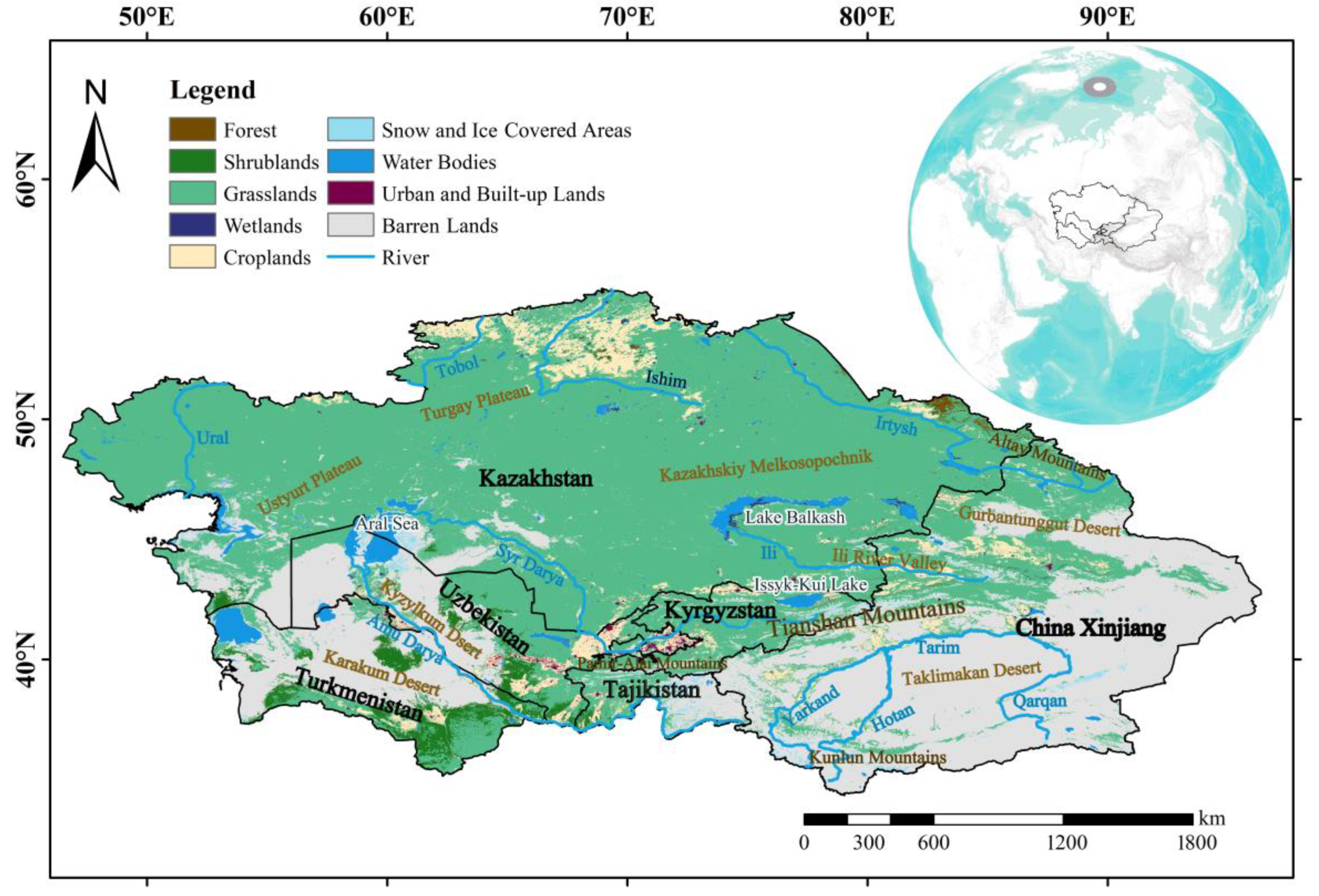
This study uses the GEE platform to explore the analysis of spatial and temporal variability of WUE in Central Asia, using both geographic detector analysis and partial correlation analysis to explore the mechanisms driving WUE in Central Asia (Figure 1).

2.1. Study Area

Central Asia is located in the hinterland of the central Asian continent and is the largest non-zoned arid zone in the world. Central Asia covers an area of approximately 5.66 million square kilometers and includes (Figure 2). Kazakhstan, Uzbekistan, Kyrgyzstan, Tajikistan, Turkmenistan, and the Xinjiang Uyghur Autonomous Region of China. The topography of Central Asia is complex, dominated by plains, basins, mountains, and deserts, with deserts and the Gobi accounting for the largest proportion of the area, forming a unique ice-snow-alpine meadow-forest-steppe-oasis-desert eco-climatic pattern. Central Asia is a temperate desert with a continental steppe climate featuring marked temperature differences, abundant light, low precipitation, and high evaporation. Water resources in Central Asia are mainly derived from precipitation, especially water vapor brought by westerly circulation. Central Asia is rich in vegetation, but vegetation cover is sparse and dominated by desert vegetation and grasslands. The largest ecosystem types in Central Asia are temperate grasslands, savannas, and sparse shrublands. Other ecosystems include montane grasslands and sparse shrubs, deserts and dense shrubs, and temperate coniferous forests.

2.2. Data Acquisition and Processing

This study uses GPP (MOD17A2) and ET (MOD16A2) to calculate WUE with a spatial resolution of 500 m and a temporal resolution of 8 days. The time span was from 2001 to 2021, and data from April–October of each year were selected. MOD17A2H Version 6 (GPP) and MOD16A2 Version 6 (ET) are the accumulated values of the eight-day composite cycle. Urban and built-up lands, water bodies, snow and ice covered areas and desert areas are almost devoid of vegetation and these areas lack GPP and ET data, so these areas are masked.

The driver data in this study included atmospheric factors (TEM, RN, LST, VPD, DEF, VAP, AOD, TSVEG), hydrological factors (PRE, VSW1, GWS, RTZSM, SFSM, PDSI, RO, SW), and biological factors (CRSI, LAI, EVI, FVC). They are expressed using the average of April–October data for each year from 2001 to 2021. Specifically, TEM (surface 2-m temperature), PRE (precipitation accumulation), and SW (soil water (0–7 cm)) data were extracted from ERA5, RN (net radiation) data were calculated from longwave net radiation, and shortwave net radiation was extracted from ERA5. AOD (550 nm thickness) was extracted from MCD19A2. VPD, water pressure (VAP), climatic water deficit (DEF), runoff (RO), soil moisture (SW), and drought index (PDSI) were obtained from TERRACLIMATE. Transpiration (TSVEG) was obtained from NOAH. LST was obtained from MOD11A2. Enhanced Vegetation Index (EVI) was obtained from MOD13Q1. FVC was calculated from Normalized Difference Vegetation Index (NDVI) data for MOD13Q1. The canopy salinity index (CRSI) was calculated from MOD09A1 data [41]. We used the groundwater content, soil moisture in the root zone (RTZSM), and surface soil moisture (SFSM) to characterize the distribution of groundwater. Specific data are detailed in

Table 1. Description of data and variables.

Factor	Data	Type	Data Description	Spatial Resolution	Time Resolution	Data Source
1	GPP		Gross primary productivity (kgC·m−2·8 day−1)	500 m	8 days	Google Earth Engine LP DAAC—MOD17A2H (usgs.gov) https://lpdaac.usgs.gov/products/mod17a2hv006/, accessed on 13 December 2022
2	ET		Total evapotranspiration (kg C·m−2·8 day−1)	500 m	8 days	Google Earth Engine LP DAAC—MOD16A2 (usgs.gov) https://lpdaac.usgs.gov/products/mod16a2v006/, accessed on 13 December 2022
X1	TEM	Atmospheric factor	Temperature_2m (k)	11,132 m	Monthly	Google Earth Engine Copernicus Climate Data Store| https://cds.climate.copernicus.eu/#!/home, accessed on 13 December 2022
X2	PRE	Hydrological factor	Total precipitation (m)	11,132 m	Monthly
X3	RN	Atmospheric factor	Resultant of the surface net solar and thermal radiation data (J/m2)	11,132 m	Monthly
X4	VSW1	Hydrological factor	Volumetric soil water content (0–7 cm depth) (m3/m3)	11,132 m	Monthly
X5	CRSI	Biological factor	$\mathrm{Canopy}\mathrm{Response}\mathrm{Salinity}\mathrm{Index}\sqrt{\frac{nir\ast red-green\ast blue}{nir\ast red+green\ast blue}}$	500 m	8 days	Google Earth Engine LP DAAC—MOD09A1 (usgs.gov) https://lpdaac.usgs.gov/products/mod09a1v006/, accessed on 13 December 2022
X6	LAI	Biological factor	Leaf Area Index	500 m	8 days	Google Earth Engine LP DAAC—MOD15A2H (usgs.gov) https://lpdaac.usgs.gov/products/mod15a2hv006/, accessed on 13 December 2022
X7	EVI	Biological factor	Enhanced Vegetation Index	250 m	16 days	Google Earth Engine LP DAAC—MOD13Q1 (usgs.gov) https://lpdaac.usgs.gov/products/mod13q1v006/, accessed on 13 December 2022
X8	FVC	Biological factor	Vegetation cover	250 m	16 days
X9	LST	Atmospheric factor	Day land surface temperature	1000 m	8 days	Google Earth Engine LP DAAC—MOD11A2 (usgs.gov) https://lpdaac.usgs.gov/products/mod11a2v006/, accessed on 13 December 2022
X10	AOD	Atmospheric factor	Green band (0.55 nm) aerosol optical depth over land	1000 m	8 days	Google Earth Engine LP DAAC—MCD19A2 (usgs.gov) https://lpdaac.usgs.gov/products/mcd19a2v006/, accessed on 13 December 2022
X11	GWS	Hydrological factor	Groundwater percentile (%)	0.25 degree	7 days	Global Data Archive|NASA Grace (unl.edu) https://nasagrace.unl.edu/GlobalData.aspx, accessed on 13 December 2022
X12	RTZSM	Hydrological factor	Root zone soil moisture percentile (%)	0.25 degree	7 days
X13	SFSM	Hydrological factor	Surface soil moisture percentile (%)	0.25 degree	7 days
X14	DEF	Atmospheric factor	Climate water deficit (mm)	4638.3 m	Monthly	Google Earth Engine TerraClimate—Climatology Lab https://www.climatologylab.org/terraclimate.html, accessed on 13 December 2022
X15	PDSI	Hydrological factor	Palmer Drought Severity Index	4638.3 m	Monthly
X16	RO	Hydrological factor	Runoff (mm)	4638.3 m	Monthly
X17	SW	Hydrological factor	Soil moisture (mm)	4638.3 m	Monthly
X18	VAP	Atmospheric factor	Vapor pressure (kPa)	4638.3 m	Monthly
X19	VPD	Atmospheric factor	Vapor-pressure deficit (kPa)	4638.3 m	Monthly
X20	TSVEG	Atmospheric factor	Transpiration (W/m2)	27,830 m	Monthly	Google Earth Engine GES DISC (nasa.gov) https://disc.gsfc.nasa.gov/datasets/GLDAS_NOAH025_3H_2.1/summary, accessed on 13 December 2022

.

2.3. WUE

This study calculated WUE based on the GEE platform. WUE (gCkg⁻¹H₂O) is defined as the ratio of MOD17A2H (GPP) to MOD16A2 (ET) every 8 days.

$$WUE=\frac{GPP}{ET}$$

(1)

Therefore, WUE was calculated using GPP (MOD17A2H) and ET (MOD16A2) for April–October each year within Central Asia for the 2001–2021 period. The average WUE for each year was calculated as the average of the WUE calculated for each year with an 8-day compound cycle. The monthly average WUE for the study period was calculated as the average of the WUE calculated for the same months in the 21 years with an 8-day compound cycle. Similarly, the average GPP and ET for each year, as well as the average monthly GPP and ET for the study period, were calculated.

2.4. Temporal Information Entropy

Temporal information entropy can highlight the intensity of change in information about a research target over a certain period of time. Time series information entropy, on the other hand, can indicate the trend of changes in information about a research target over a certain period of time [42,43]:

$$T=\frac{1}{n}{\displaystyle \sum {}_{i=q}^n{\log }_2\frac{y_{i+m}-y_{i-m}}{c_i\times \mathrm{m}\times △/\mathrm{n}}}$$

(2)

$$T_{c_i}=\left\{\begin{array}{l}1+\frac{i-1}{m},1\le i\le m\\ 2,m+1\le i\le n-m\\ 1+\frac{n-i}{m},n-m+1\le i\le n\end{array}\right.$$

(3)

$$\left\{\begin{array}{l}{y}_{i-m}=y_i,i\le m\\ y_{i+m}=y_n,i\ge n-m\end{array}\right.$$

(4)

where $T$ is the value of temporal information entropy, $y_1\le y_2\le \cdots \le y_n$, $y_i$ is the WUE value in year i of any image element $x_i$ in order from smallest to largest, m is the temporal frequency of the WUE calculation, $m<n/2, m\in \mathbb{Z}+$, and ∆ is the scaling factor. In this paper, we use April–October each year as the growing season to represent the year as a whole, so m = 1 and ∆ = 0.02:

$$T^{\prime }=\frac{1}{n}\mathrm{sgn}\left(x_{i+m}-x_{i-m}\right){\displaystyle \sum {}_{i=1}^n\log \left(\frac{\left|x_{i+m}-x_{i-m}\right|}{c_i\times \mathrm{m}\times △/n}\right)}$$

(5)

where $T^{\prime }$ is the value of time series information entropy, $x_i$ is the WUE value for year i of any image element, and $sgn$ is a symbolic function, $sgn\left(\theta \right)=\left\{\begin{array}{c}1,\theta >0\\ 0,\theta =0\\ -1,\theta <0\end{array}\right.$. The other parameters are defined and valued as above.

2.5. Geographical Detector

Geographical detectors are statistical methods for detecting geographical divergence and exploring driving forces [44]. The geographical detector model contains four modules, namely, the factor detector, interaction detector, risk detector, and ecological detector. In this paper, we used the factor detector, interaction detector, and ecological detector to explore the driving mechanism of WUE. Among these, factor detectors can detect the extent to which different drivers drive the spatial differentiation of the study target. In this paper, we used factor detectors to detect the extent to which 20 drivers contribute to WUE. The explanatory power of each driver is represented by a value of $q$, where $q\in \left[0,1\right]$. A higher value of q indicates a stronger effect of the driver:

$$\mathrm{q}=1-\frac{{\displaystyle \sum {}_{h=1}^L{N}_h{\sigma }_h{}^2}}{N{\sigma }^2}=1-\frac{SSW}{SST}$$

(6)

where $L$ is the classification or partitioning of WUE or various drivers. $N_h$ and $\mathcal{N}$ represent the number of cells in the stratified region ($n$) and the whole region ($N$), respectively. ${\sigma }_h{}^2$ and ${\sigma }^2$ represent the variance of the stratified WUE in region h and the variance of the whole region WUE, respectively, and SSW and SST are the within sum of squares and total sum of squares, respectively [45].

Ecological detection determines whether there is a significant difference in the spatial distribution of WUE between the two drivers by means of an F-test. Interaction detection is used to identify whether the interaction between drivers enhances or diminishes the degree of explanation of WUE by comparing the q-value between the two drivers with that of the interaction. In this paper, we can use interaction detection to explore the degree of explanation of the combination of drivers on WUE.

3. Results

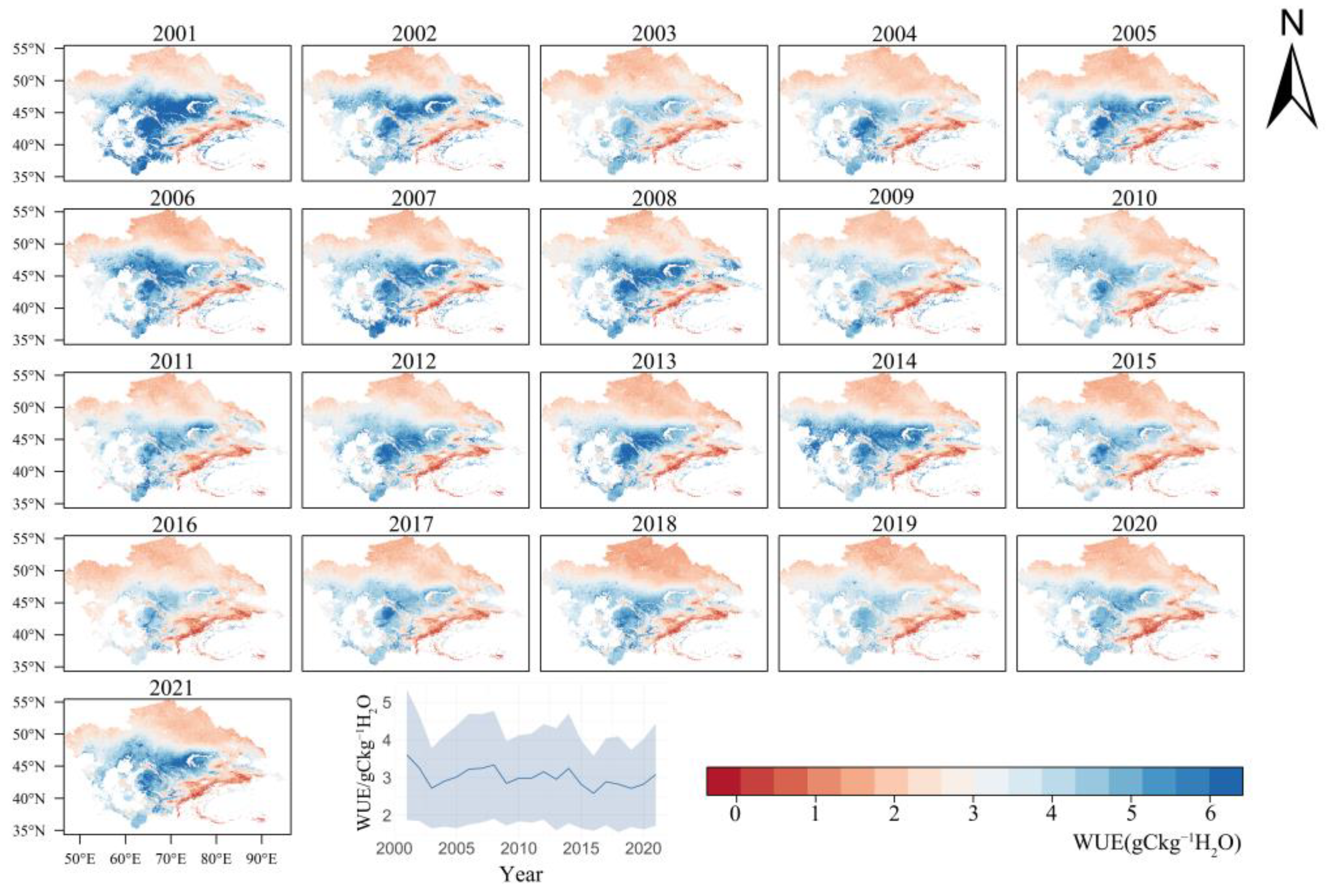
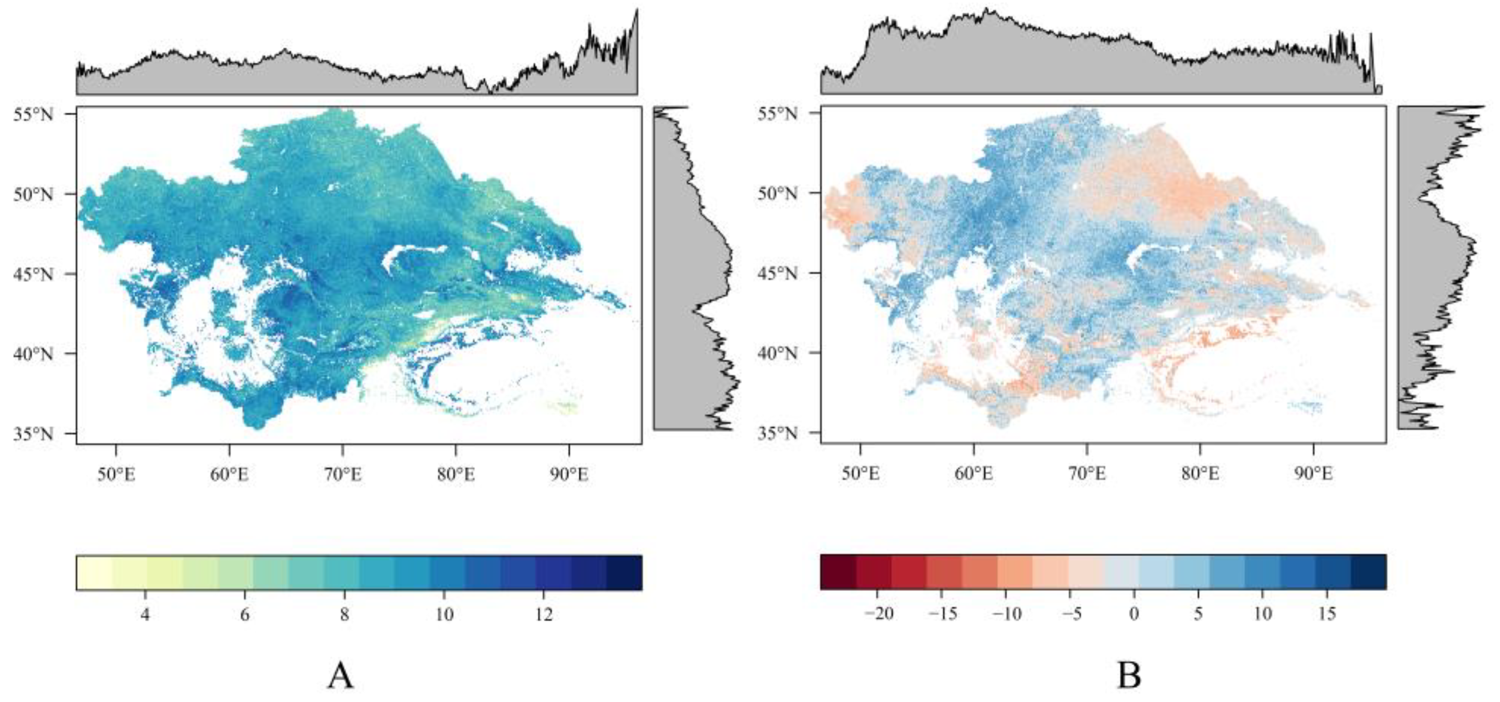
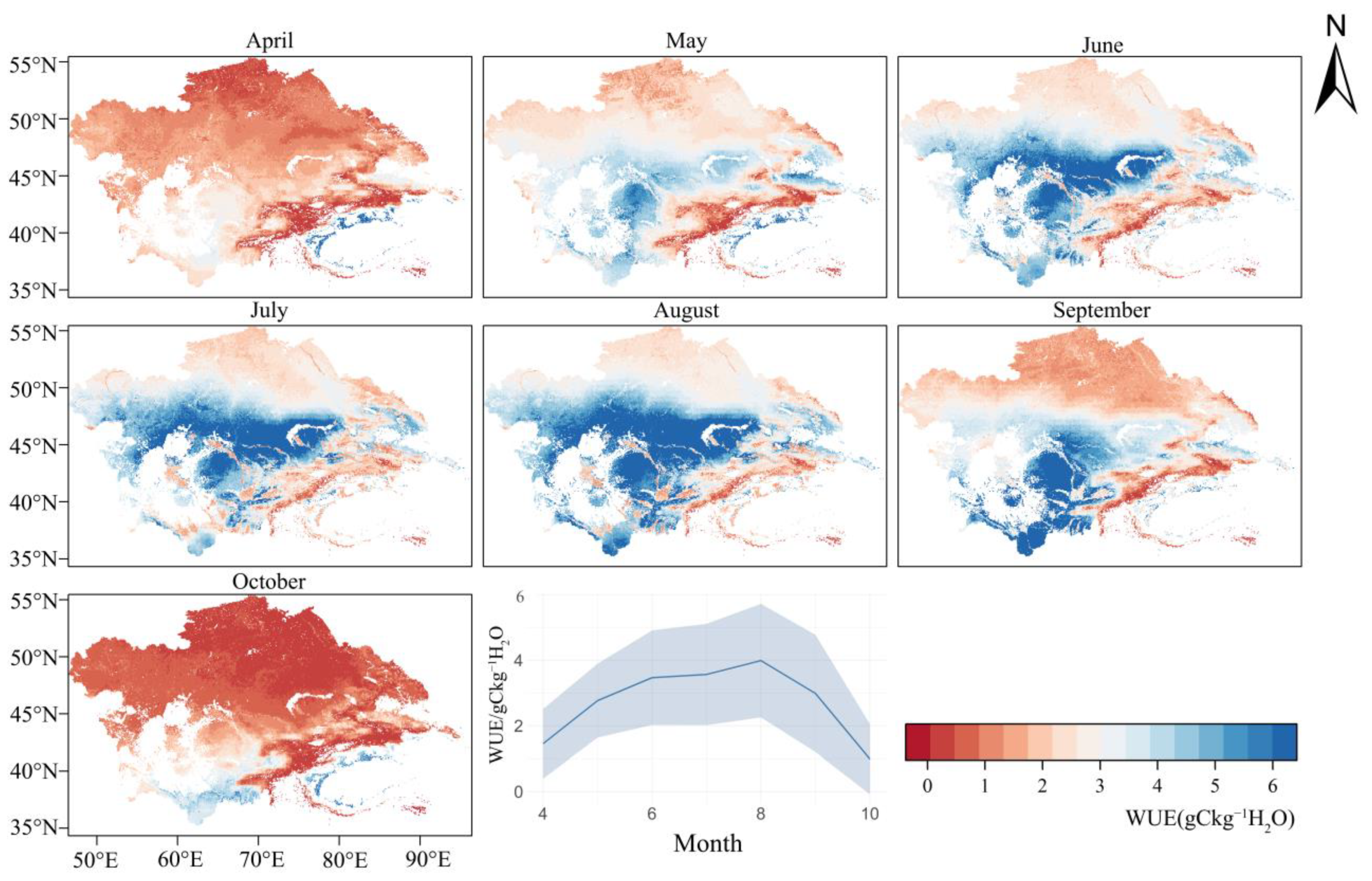
3.1. Spatial and Temporal Variation of WUE

The yearly spatial and temporal distribution of the annual average WUE in Central Asia in 2001–2021 is shown in Figure 3. The average WUE value during 2001–2021 is 3.011 gCkg⁻¹H₂O, with an overall trend of WUE decreasing in Central Asia by a small amount per year. The spatial heterogeneity of WUE is evident in the spatial variability, with high WUE values concentrated in the Aral Sea periphery to the Lake Balkhash Basin in southern Kazakhstan, northeastern Uzbekistan to the Syr Darya Basin, the southern edge of Turkmenistan, the southern edge of the Tian Shan Mountains, and the northern edge of the Tian Shan Mountains. The medium-WUE areas are concentrated in the Ural, Tobol, Ishim, and Erzis river basins in northern Kazakhstan. The most pronounced spatial and temporal variation is found in the high-WUE areas, indicating that the arid ecology of Central Asia has a strong and persistent influence on the high-WUE areas, and that the adaptation of the region to arid ecology has led to consistently high WUE values.

3.2. Time Series Variation of Annual Average WUE

The temporal information entropy and time series information entropy of WUE in Central Asia in 2001–2021 are shown in Figure 4. The intensity of WUE change in Central Asia as a whole over the past 21 years is high, with significant decreases in WUE in the southern margin of Turkmenistan, the oases in eastern Uzbekistan, southwestern Tajikistan, and the oases around the Gurbantunggut and Taklamakan deserts, and significant increases in WUE in the Ustyurt Plateau, around the Aral Sea to the Lake Balkhash Basin, the Ili Valley, and central and western Tajikistan. The results indicate that although the annual mean variation is weak, the spatial distribution changes significantly, and more oases show a decreasing trend in WUE.

3.3. Analysis of the Impact of Driving Factors

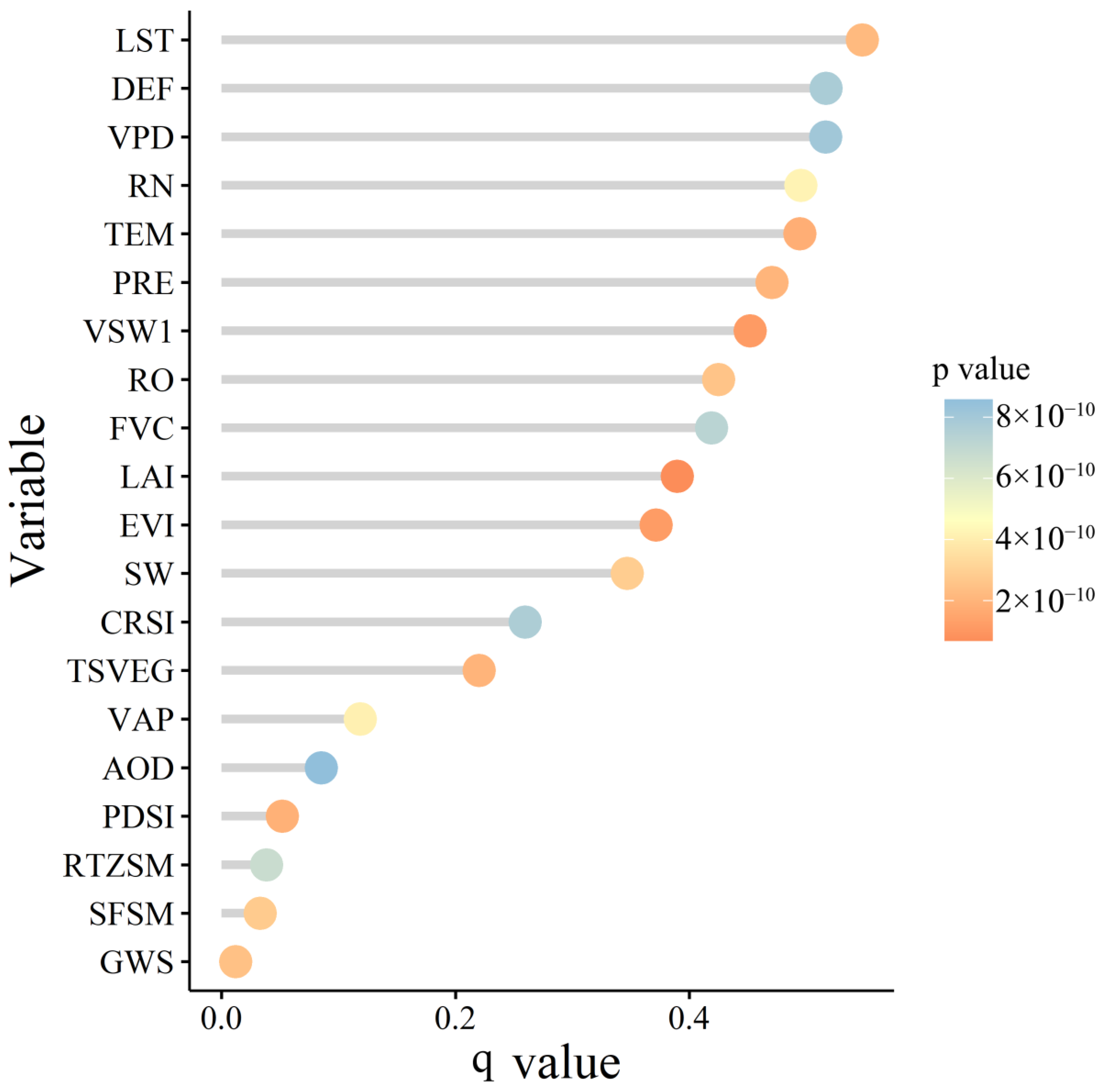
3.3.1. Detection Factor Influence

The factor detection results of the impact of each driver on WUE are shown in Figure 5. All drivers passed the significance test (p = 0.001) from 2001 to 2021. The factor analysis shows that LST has a dominant effect on WUE (q = 0.548), and GWS has the least driving effect on WUE (q = 0.012). LST, DEF, VPD, RN, TEM, PRE, and VSW1 have a high degree of influence on WUE, explaining more than 45% of the variation in WUE. VAP, AOD, PDSI, and GWS have a low degree of influence on WUE, explaining less than 20% of the variation.

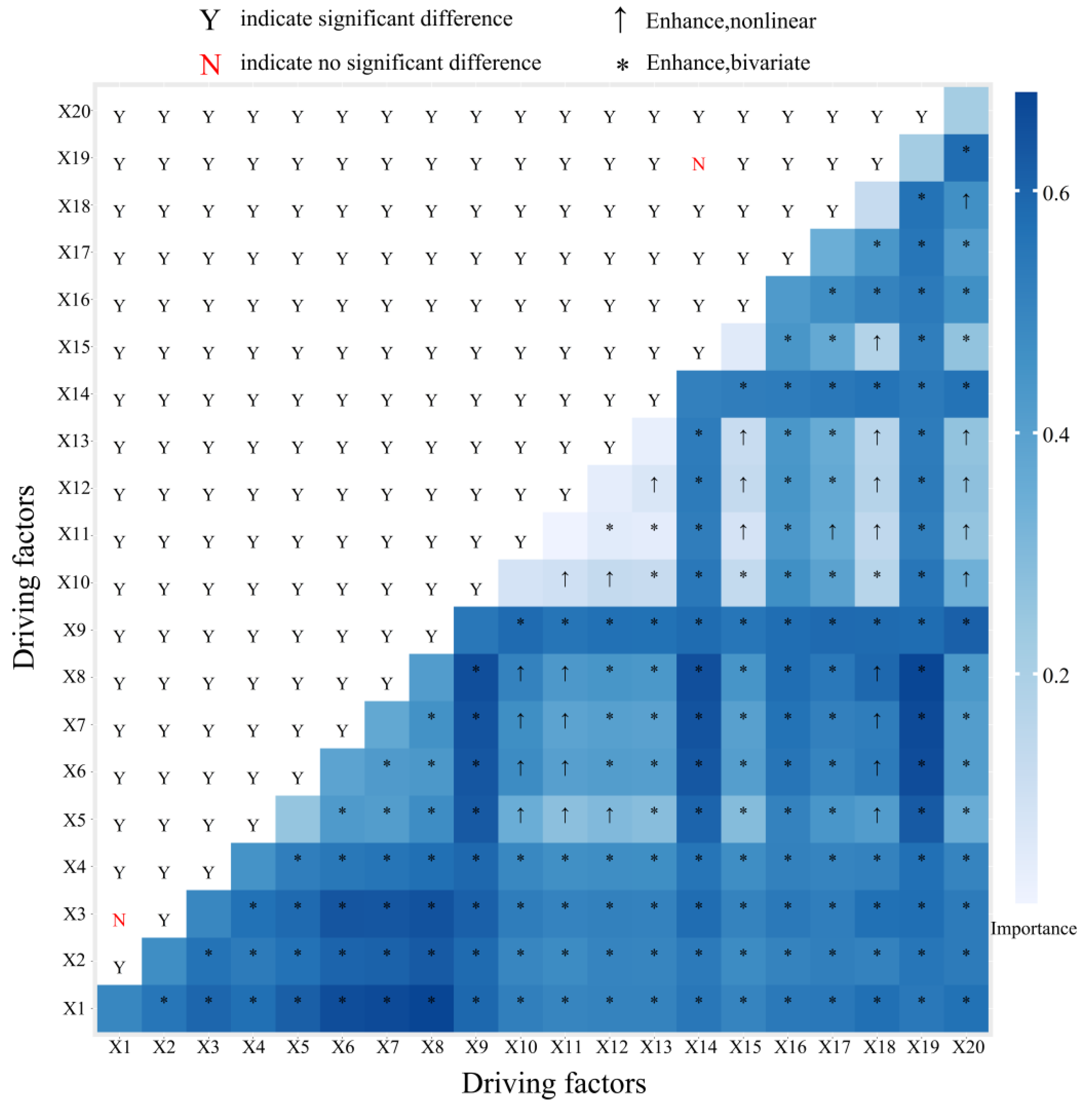
3.3.2. Statistics of Significant Differences between Drivers and Interactions

The results of the ecological detection and interactive detection are shown in Figure 6. The ecological detection shows that there is no significant difference in the spatial distribution of WUE between the TEM and RN, DEF, and VPD natural factors. There is a significant difference in the spatial distribution of WUE between all the remaining drivers affecting WUE. The interactions between the drivers were then explored to investigate their driving effect on WUE. The interaction between $\mathrm{X}1$ and $\mathrm{X}8$ (X1 ∩ X8 (0.681) > Max (q(X1(0.496)), q(X8(0.419)))) is bilinearly enhanced, with X1 and X8 synergistically explaining each other’s WUE changes most strongly; the interaction of the two explained 68.1% of the variation in WUE. Specifically, $\mathrm{TEM}\cap \mathrm{FVC}\left(\mathrm{X}1\cap \mathrm{X}8,\mathrm{q}=0.681\right)$, $\mathrm{TEM}\cap \mathrm{CRSI}\left(\mathrm{X}1\cap \mathrm{X}5,\mathrm{q}=0.615\right)$, $\mathrm{TEM}\cap \mathrm{LAI}\left(\mathrm{X}1\cap \mathrm{X}6,\mathrm{q}=0.661\right)$, $\mathrm{TEM}\cap \mathrm{EVI}\left(\mathrm{X}1\cap \mathrm{X}7,\mathrm{q}=0.668\right)$, $\mathrm{PRE}\cap \mathrm{LAI}\left(\mathrm{X}2\cap \mathrm{X}6,\mathrm{q}=0.601\right)$, $\mathrm{PRE}\cap \mathrm{EVI}\left(\mathrm{X}2\cap \mathrm{X}7,\mathrm{q}=0.606\right)$, $\mathrm{PRE}\cap \mathrm{FVC}\left(\mathrm{X}2\cap \mathrm{X}8,\mathrm{q}=0.627\right)$, $\mathrm{TEM}\cap \mathrm{FVC}\left(\mathrm{X}1\cap \mathrm{X}8,\mathrm{q}=0.681\right)$, $\mathrm{RN}\cap \mathrm{LAI}\left(\mathrm{X}3\cap \mathrm{X}6,\mathrm{q}=0.639\right)$, $\mathrm{RN}\cap \mathrm{EVI}\left(\mathrm{X}3\cap \mathrm{X}7,\mathrm{q}=0.636\right)$, $\mathrm{RN}\cap \mathrm{FVC}\left(\mathrm{X}3\cap \mathrm{X}8,\mathrm{q}=0.648\right)$, $\mathrm{RN}\cap \mathrm{LST}\left(\mathrm{X}3\cap \mathrm{X}9,\mathrm{q}=0.611\right)$, $\mathrm{CRSI}\cap \mathrm{LST}\left(\mathrm{X}5\cap \mathrm{X}9,\mathrm{q}=0.629\right)$, $\mathrm{CRSI}\cap \mathrm{DEF}\left(\mathrm{X}5\cap \mathrm{X}14,\mathrm{q}=0.601\right)$, $\mathrm{CRSI}\cap \mathrm{VPD}\left(\mathrm{X}5\cap \mathrm{X}19,\mathrm{q}=0.628\right)$, $\mathrm{LAI}\cap \mathrm{LAI}\left(\mathrm{X}6\cap \mathrm{X}9,\mathrm{q}=0.637\right)$, $\mathrm{LAI}\cap \mathrm{DEF}\left(\mathrm{X}6\cap \mathrm{X}14,\mathrm{q}=0.635\right)$, $\mathrm{LAI}\cap \mathrm{VPD}\left(\mathrm{X}6\cap \mathrm{X}19,\mathrm{q}=0.662\right)$, $\mathrm{EVI}\cap \mathrm{LST}\left(\mathrm{X}7\cap \mathrm{X}9,\mathrm{q}=0.644\right)$, $\mathrm{EVI}\cap \mathrm{DEF}\left(\mathrm{X}7\cap \mathrm{X}14,\mathrm{q}=0.645\right)$, $\mathrm{EVI}\cap \mathrm{VPD}\left(\mathrm{X}7\cap \mathrm{X}19,\mathrm{q}=0.668\right)$, $\mathrm{FVC}\cap \mathrm{LST}\left(\mathrm{X}8\cap \mathrm{X}9,\mathrm{q}=0.657\right)$, $\mathrm{FVC}\cap \mathrm{DEF}\left(\mathrm{X}8\cap \mathrm{X}14,\mathrm{q}=0.655\right)$, $\mathrm{FVC}\cap \mathrm{VPD}\left(\mathrm{X}8\cap \mathrm{X}19,\mathrm{q}=0.678\right)$, and $\mathrm{LST}\cap \mathrm{TSVEG}(\mathrm{X}9\cap \mathrm{X}20,\mathrm{q}=0.611$. The interactions of the above 24 driver combinations all explained more than 60% of the variation in WUE, indicating that 11 drivers—TEM, PRE, RN, CRSI, LAI, EVI, FVC, LST, DEF, TSVEG, and VPD—dominated the explanation of WUE variation in the bilinear enhancement type. Of these, the vegetation factors LAI, EVI, FVC, and CRSI occupied 22 combinations with the six drivers TEM, PRE, RN, LST, DEF, and VPD, so the vegetation factors were the most important among the bilinear enhancement effects.

In addition, the relationship between X8 and X18 (X8 ∩ X18(0.592) > 0.542 = X8(0.419) + X18(0.123)) was non-linearly strengthened. X8 and X18 strengthened each other’s ability to explain changes in WUE; their interaction explains 59.2% of the change in WUE. There were also 29 other combinations of X18 and X20, X6 and X18, X7 and X18, X6 and X10, X7 and X10, X8 and X10, X6 and X11, X7 and X11, X8 and X11, and other drivers with the same type of effect. Specifically, $\mathrm{FVC}\cap \mathrm{VAP}\left(\mathrm{X}8\cap \mathrm{X}18,\mathrm{q}=0.592\right)$,$\mathrm{VAP}\cap \mathrm{TSVEG}\left(\mathrm{X}18\cap \mathrm{X}20,\mathrm{q}=0.463\right)$, $\mathrm{LAI}\cap \mathrm{VAP}\left(\mathrm{X}6\cap \mathrm{X}18,\mathrm{q}=0.534\right)$, $\mathrm{EVI}\cap \mathrm{VAP}\left(\mathrm{X}7\cap \mathrm{X}18,\mathrm{q}=0.529\right)$, $\mathrm{LAI}\cap \mathrm{AOD}\left(\mathrm{X}6\cap \mathrm{X}10,\mathrm{q}=0.479\right)$,$\mathrm{EVI}\cap \mathrm{AOD}\left(\mathrm{X}7\cap \mathrm{X}10,\mathrm{q}=0.469\right)$,$\mathrm{FVC}\cap \mathrm{AOD}\left(\mathrm{X}8\cap \mathrm{X}10,\mathrm{q}=0.512\right)$,$\mathrm{LAI}\cap \mathrm{GWS}\left(\mathrm{X}6\cap \mathrm{X}11,\mathrm{q}=0.404\right)$, $\mathrm{EVI}\cap \mathrm{GWS}\left(\mathrm{X}7\cap \mathrm{X}11,\mathrm{q}=0.390\right)$, and $\mathrm{FVC}\cap \mathrm{GWS}\left(\mathrm{X}8\cap \mathrm{X}11,\mathrm{q}=0.432\right)$. The interaction between vegetation factors LAI, EVI, and FVC with VAP, AOD, GWS, TSVEG, and VAP was shown to be the strongest in explaining WUE. For example, as shown in Figure 4, VAP and TSVEG were weaker in explaining WUE changes (q = 0.123 and q = 0.220). However, the interaction between VAP and TSVEG explained 46.3% (q = 0.463) of the change in WUE. This result indicates that some drivers with low driving effects were influenced by other drivers, with such interactions rapidly increasing the driving effect. Therefore, considering the interaction between different factors allows the identification of driving mechanisms with greater explanatory power for WUE. Among these, the combination of VAP with each of the nine drivers was non-linearly enhanced. The combination of vegetation factors LAI, EVI, and FVC, interacting with AOD, GWS, and SW, explained 39.0–59.2% of the variation in WUE. The combined driving effect of the vegetation factors was the strongest of the two effect types.

4. Discussion

4.1. Spatial and Temporal Variation and Distribution of WUE in Central Asia

It has been shown that the results of ecosystem WUE calculations based on the MODIS products GPP and ET are highly consistent with calculations based on flux tower data [20,24]. Based on the MODIS products GPP and ET, Xue et al. and Huang et al. obtained a global mean annual WUE of 1.7 gCkg⁻¹H₂O [24,26]. Using the same methodology, the mean annual value of WUE in this study is 3.011 gCkg⁻¹H₂O, which is similar to other ranges calculated in dryland areas, such as southern and northern Africa, Australia, and central South America, where the WUE of dryland ecosystems ranges from 2.5 gCkg⁻¹H₂O to 5.1 gCkg⁻¹H₂O [26]. In addition, the estimation of WUE based on the Google Earth platform significantly improved the efficiency of the study. The WUE of dryland ecosystems is higher than the global average due to the fact that vegetation in dryland ecosystems experiences long periods of drought and is more tolerant of dry conditions [46]. Vegetation in dryland ecosystems is more sensitive to climatic factors [32,47]. Therefore, WUE monitoring and assessment of dryland ecosystems can contribute to a more comprehensive understanding of changes in the carbon–water cycle in dryland ecosystems and enhance the ability to predict future climate change [11].

We found weak inter-annual variability in WUE in Central Asia, with significant intra-annual variability and some seasonality (Figure 7). This is evidenced by an increase from April to a maximum in August each year, followed by a rapid decline, which is consistent with the conclusions obtained by Zou et al. and Subrata et al. [27,28]. High WUE is mainly concentrated in June, July, and August due to reduced transpiration and reduced water consumption due to the partial closure of natural vegetation stomata during the dry season [48]. In contrast, relatively adequate artificial irrigation means that crops are relatively less affected by drought stress. However, artificial irrigation causes significant evaporation of soil water, which, in turn, leads to a lower WUE for the crops [49]. It is noteworthy that the areas of Central Asia where inter-annual variation in WUE declined significantly were also concentrated in oases, possibly due to irrigation practices on arable land and irrational cropping structures during the monitored period. For example, Zou et al. found that the irrigated areas of Uzbekistan, Turkmenistan, and the southern oases of Xinjiang, China were agricultural, and that the main crop during the monitoring period was cotton, which is a high water consumer [27]. Therefore, the conservation of dryland ecosystems requires a rational allocation of water resources and a trade-off between agricultural and ecological uses. It is not necessarily a good thing that crops in oases are over-irrigated, which reduces the efficiency of water use and also causes soil salinization [50,51]; therefore, it is important to protect the ecosystem while ensuring food production security. In addition, this study found a significant increase in WUE in Central Asia in the Ustyurt Plateau, around the Aral Sea to the Lake Balkhash Basin, the Ili River Basin, and in central Tajikistan. It has been shown that the Ustyurt Plateau experiences long periods of drought, which, in turn, strengthens the drought resistance of the vegetation in the area [52], thereby increasing WUE [27]. Liu et al. found that the increasing trend of actual net primary productivity (ANPP) in the Lake Balkhash Basin and the Ili River Basin was due to appropriate grazing and progressively warmer and wetter climate change in the basin. Not only has the climate in the basin become suitable for vegetation growth, but grazing intensity has also been reduced [53], which may lead to an increase in WUE in the region. Although the overall inter-annual variability in Central Asia is not strong, the spatial distribution is highly variable in intensity. Therefore, exploring the spatial and temporal variability of WUE in Central Asia can improve our understanding of the magnitude of long-term WUE variation and long-term trends in Central Asia, allowing the optimization of water resource management.

4.2. Driving Mechanisms of WUE Change in Central Asia

Based on the geographic detector, we can not only assess the importance of the drivers quickly and effectively, but can also determine the importance of the interactions between drivers. In contrast to linear regression, the geographic detector works with continuous data and is not limited by multicollinearity [54]. In addition, through partial correlation analysis, we can determine the direction of correlation between drivers and GPP, ET, and WUE. We found that the atmospheric factors LST, DEF, VPD, RN, and TEM have a significant effect on WUE in Central Asia. Among these, LST has the strongest driving role and can explain 54.8% of the variation in WUE. The above five atmospheric factors correlate negatively with GPP and ET in most parts of Central Asia and positively with WUE (Figure 8). In contrast, the hydrological factors PRE and VSW1 correlate positively with GPP and ET and negatively with WUE in most of Central Asia (Figure 8). Because increases in LST and TEM cause drought, and the correlation between LST and VPD is high [34], both drought and high VPD promote the stomatal closure of plant leaves, leading to a decrease in evapotranspiration before a decrease in photosynthesis rate, causing an increase in WUE [55,56]. Furthermore, with strong evapotranspiration in Central Asia, water in the soil evaporates rapidly after precipitation occurs, which, in turn, limits the ability of vegetation to absorb CO₂. For example, Xue et al. found that WUE in sparsely vegetated and drier areas increased with decreasing precipitation [24]. We found that the seven drivers mentioned above explain WUE in Central Asia to a high degree, and all drive WUE by affecting vegetation photosynthesis or transpiration.

We found that the interactions between the 20 selected drivers all strongly enhance the driving force on WUE, suggesting responses between drivers can better explain changes in WUE. A total of 22 interactions between atmospheric and vegetation factors explained more than 60% of the variation in WUE. The vegetation factors CRSI, LAI, EVI, and FVC were all positively correlated with GPP and ET and negatively correlated with WUE (Figure 8). It has been shown that Central Asia is turning green and that the recovery of vegetation leads to a significant increase in GPP and ET [23,38]. However, under drought stress, vegetation regulates its own water consumption mechanisms by reducing leaf area [36], reflecting the physiological adaptation of vegetation to water stress [57,58]. It has also been suggested that increasing LAI may lead to stronger evapotranspiration than transpiration, resulting in a decrease in WUE [37]. This study likewise found that transpiration under climate stress could explain WUE changes well; for example, the combination of VAP and TSVEG drove a 12% increase in capacity. In addition, the interaction between AOD and GWS can substantially enhance the driving force, especially the interaction with vegetation factors, which has the most significant enhancement effect. It has been shown that aerosols can form foliar dust that affects the photosynthesis of vegetation, and that appropriate groundwater levels are beneficial to the growth of vegetation in arid zones [38,59]. We found that vegetation factors are the most critical aspects of WUE change in Central Asia, with FVC being the strongest driving vegetation factor. Integrating the effects of aerosol and groundwater distribution on vegetation can provide a better understanding of WUE change in Central Asia. In summary, atmospheric and hydrological factors drive changes in WUE through their effects on vegetation photosynthesis and transpiration. Both atmospheric and hydrological factors have a strong interactive driving effect with vegetation factors. Vegetation is the most important factor driving WUE in Central Asia, but vegetation cover is inversely related to WUE, with an increase in vegetation cover leading to greater evapotranspiration than transpiration. It has also been shown that an increase in vegetation cover in Central Asia will lead to a decrease in surface water availability due to increased evapotranspiration, which suggests that a series of measures to rapidly promote ecological restoration could accelerate the depletion of water availability [60,61]. However, the ecological environment in Central Asia is very fragile, and a prerequisite for improving its quality is to prevent it from deteriorating further. Through controlling grazing, we should increase the protection of existing vegetation and reduce deforestation caused by human activities [62]. Therefore, ecological restoration in Central Asia needs to be carried out gradually and slowly, and priority should be given to vegetation that is adapted to the atmospheric and hydrological conditions of Central Asia.

4.3. Uncertainty and Future Work

In this study, the MODIS products GPP and ET were used to calculate the WUE for Central Asia from 2001 to 2021, with annual averages in the range of 2.584–3.607 gCkg⁻¹H₂O, similar to previous studies. However, the calculation of WUE in arid areas from MODIS data led to an underestimation [25,63,64,65]. This result is inevitable due to the underestimation of ET from MODIS data in arid areas, which may lead to some uncertainty in the calculation results. Similarly, this study did not consider vegetation eaten by grazing animals, leading to a certain underestimation of GPP and ET. Uncertainty in the calculation of WUE based on MODIS is usually acceptable; for example, Tang et al. validated the results of the MODIS calculation of WUE with the help of flux tower data (32 sites), with R² values ranging from 0.74 to 0.963 for different vegetation types [20]. Furthermore, the WUE of Central Asia in this study was calculated without considering desert, due to the sparse vegetation and exposed soil surface conditions in arid areas. The normalized difference vegetation index (NDVI) based on remote sensing data does not reflect surface vegetation conditions. The MODIS products GPP and ET, which are estimated based on NDVI, also deviate from the real values in deserts, so not considering deserts improves the reliability of the results to some extent [27]. Studies are increasingly using flux data in combination with remote sensing data to quantify research at regional to global scales. The main problem in Central Asia is the great lack of long-term flux tower data, and this study could only use MODIS data to calculate WUE. In addition, it was not possible to establish empirical relationships between WUE and each explanatory variable by training with rich data. Therefore, the network of dryland covariance flux tower observations needs to be expanded in the future to provide data support for the development of dryland-specific models [10]. Changes in carbon and water fluxes in dryland ecosystems are more specific and less predictable than in other ecosystems [66]. This study demonstrates the importance of the interaction between atmospheric and vegetation factors in driving WUE in Central Asia, and the increased awareness of climate change and the development of appropriate ecological restoration policies may facilitate the planting of environmentally adaptive vegetation and, thus, the maintenance and development of available water resources in Central Asia. Our results can be used to improve future climate change prediction ability, optimize water resources management, and safeguard food production.

5. Conclusions

This study calculated the WUE of Central Asia for 2001–2021 using the GEE platform based on the MODIS products GPP and ET. The driving mechanisms of atmospheric, hydrological, and biological factors on the WUE of Central Asia were analyzed using a geographic detector. The results show that the mean value of WUE is 3.011 gCkg⁻¹H₂O, with a weak inter-annual variation and an overall decreasing trend of 0.0198 gCkg⁻¹H₂O per year on average, and a clear inverted “V” shape of intra-annual variation. The spatial distribution of WUE varies significantly, with significant decreases in WUE on the southern edge of Turkmenistan, oases in eastern Uzbekistan, southwestern Tajikistan, and oases around the Gurbantungut and Taklamakan deserts, and significant increases in WUE on the Ustyurt Plateau, around the Aral Sea to the Lake Balkhash Basin, in the Ili River Basin, and in central and western Tajikistan. The atmospheric factors LST, DEF, VPD, RN, and TEM, and the hydrological factors PRE and VSW1 together explain more than 45% of the WUE in Central Asia, with LST being the strongest driver of WUE. The interaction of atmospheric factors and vegetation factors is the greatest driver of changes in WUE in Central Asia, and vegetation factors are important in both bilinearly enhanced and non-linearly enhanced types of interactions. In Central Asia, vegetation cover is inversely proportional to WUE, and FVC is the best performing vegetation index among the vegetation factors. This study also found that VAP, AOD, and GWS can enhance the drive of vegetation factors on WUE in Central Asia under the interaction of drivers. Therefore, we recommend that more attention be paid to climate change in Central Asia in the future, and advise against blind greening projects that could lead to a rapid depletion of available water resources in Central Asia.

References

1. Keenan, T.F.; Prentice, I.C.; Canadell, J.G.; Williams, C.A.; Wang, H.; Raupach, M.; Collatz, G.J. Recent pause in the growth rate of atmospheric CO2 due to enhanced terrestrial carbon uptake. Nat. Commun. 2016, 7, 13428. [Google Scholar] [CrossRef] [PubMed] [Green Version]
2. Yang, Y.; Guan, H.; Batelaan, O.; McVicar, T.R.; Long, D.; Piao, S.; Liang, W.; Liu, B.; Jin, Z.; Simmons, C.T. Contrasting responses of water use efficiency to drought across global terrestrial ecosystems. Sci. Rep. 2016, 6, 23284. [Google Scholar] [CrossRef] [PubMed] [Green Version]
3. Cheng, L.; Zhang, L.; Wang, Y.-P.; Canadell, J.G.; Chiew, F.H.S.; Beringer, J.; Li, L.; Miralles, D.G.; Piao, S.; Zhang, Y. Recent increases in terrestrial carbon uptake at little cost to the water cycle. Nat. Commun. 2017, 8, 110. [Google Scholar] [CrossRef] [PubMed] [Green Version]
4. Huang, M.; Piao, S.; Sun, Y.; Ciais, P.; Cheng, L.; Mao, J.; Poulter, B.; Shi, X.; Zeng, Z.; Wang, Y. Change in terrestrial ecosystem water-use efficiency over the last three decades. Glob. Chang. Biol. 2015, 21, 2366–2378. [Google Scholar] [CrossRef] [PubMed]
5. Keenan, T.F.; Hollinger, D.Y.; Bohrer, G.; Dragoni, D.; Munger, J.W.; Schmid, H.P.; Richardson, A.D. Increase in forest water-use efficiency as atmospheric carbon dioxide concentrations rise. Nature 2013, 499, 324–327. [Google Scholar] [CrossRef] [PubMed]
6. Ainsworth, E.A.; Long, S.P. What have we learned from 15 years of free-air CO2 enrichment (FACE)? A meta-analytic review of the responses of photosynthesis, canopy properties and plant production to rising CO2. New Phytol. 2005, 165, 351–372. [Google Scholar] [CrossRef]
7. Ahlström, A.; Raupach, M.R.; Schurgers, G.; Smith, B.; Arneth, A.; Jung, M.; Reichstein, M.; Canadell, J.G.; Friedlingstein, P.; Jain, A.K.; et al. The dominant role of semi-arid ecosystems in the trend and variability of the land CO2 sink. Science 2015, 348, 895–899. [Google Scholar] [CrossRef] [Green Version]
8. Poulter, B.; Frank, D.; Ciais, P.; Myneni, R.B.; Andela, N.; Bi, J.; Broquet, G.; Canadell, J.G.; Chevallier, F.; Liu, Y.Y.; et al. Contribution of semi-arid ecosystems to interannual variability of the global carbon cycle. Nature 2014, 509, 600–603. [Google Scholar] [CrossRef] [Green Version]
9. Schlaepfer, D.R.; Bradford, J.B.; Lauenroth, W.K.; Munson, S.M.; Tietjen, B.; Hall, S.A.; Wilson, S.D.; Duniway, M.C.; Jia, G.; Pyke, D.A.; et al. Climate change reduces extent of temperate drylands and intensifies drought in deep soils. Nat. Commun. 2017, 8, 14196. [Google Scholar] [CrossRef] [Green Version]
10. Smith, W.K.; Dannenberg, M.P.; Yan, D.; Herrmann, S.; Barnes, M.L.; Barron-Gafford, G.A.; Biederman, J.A.; Ferrenberg, S.; Fox, A.M.; Hudson, A.; et al. Remote sensing of dryland ecosystem structure and function: Progress, challenges, and opportunities. Remote Sens. Environ. 2019, 233, 111401. [Google Scholar] [CrossRef]
11. Booth, B.B.B.; Jones, C.D.; Collins, M.; Totterdell, I.J.; Cox, P.M.; Sitch, S.; Huntingford, C.; Betts, R.A.; Harris, G.R.; Lloyd, J. High sensitivity of future global warming to land carbon cycle processes. Environ. Res. Lett. 2012, 7, 024002. [Google Scholar] [CrossRef]
12. Gedney, N.; Cox, P.M.; Betts, R.A.; Boucher, O.; Huntingford, C.; Stott, P.A. Detection of a direct carbon dioxide effect in continental river runoff records. Nature 2006, 439, 835–838. [Google Scholar] [CrossRef]
13. Jackson, R.B.; Jobbágy, E.G.; Avissar, R.; Roy, S.B.; Barrett, D.J.; Cook, C.W.; Farley, K.A.; le Maitre, D.C.; McCarl, B.A.; Murray, B.C. Trading Water for Carbon with Biological Carbon Sequestration. Science 2005, 310, 1944–1947. [Google Scholar] [CrossRef] [PubMed] [Green Version]
14. Ukkola, A.M.; Prentice, I.C.; Keenan, T.F.; van Dijk, A.I.J.M.; Viney, N.R.; Myneni, R.B.; Bi, J. Reduced streamflow in water-stressed climates consistent with CO2 effects on vegetation. Nat. Clim. Chang. 2016, 6, 75–78. [Google Scholar] [CrossRef] [Green Version]
15. Beringer, J.; Hutley, L.B.; Hacker, J.M.; Neininger, B.; Paw, U.K.T. Patterns and processes of carbon, water and energy cycles across northern Australian landscapes: From point to region. Agric. For. Meteorol. 2011, 151, 1409–1416. [Google Scholar] [CrossRef]
16. Xiao, J.; Sun, G.; Chen, J.; Chen, H.; Chen, S.; Dong, G.; Gao, S.; Guo, H.; Guo, J.; Han, S.; et al. Carbon fluxes, evapotranspiration, and water use efficiency of terrestrial ecosystems in China. Agric. For. Meteorol. 2013, 182–183, 76–90. [Google Scholar] [CrossRef]
17. Xie, J.; Chen, J.; Sun, G.; Zha, T.; Yang, B.; Chu, H.; Liu, J.; Wan, S.; Zhou, C.; Ma, H.; et al. Ten-year variability in ecosystem water use efficiency in an oak-dominated temperate forest under a warming climate. Agric. For. Meteorol. 2016, 218–219, 209–217. [Google Scholar] [CrossRef]
18. Xue, Y.; Liang, H.; Zhang, B.; He, C. Vegetation restoration dominated the variation of water use efficiency in China. J. Hydrol. 2022, 612, 128257. [Google Scholar] [CrossRef]
19. He, B.; Wang, H.; Huang, L.; Liu, J.; Chen, Z. A new indicator of ecosystem water use efficiency based on surface soil moisture retrieved from remote sensing. Ecol. Indic. 2017, 75, 10–16. [Google Scholar] [CrossRef] [Green Version]
20. Tang, X.; Li, H.; Desai, A.R.; Nagy, Z.; Luo, J.; Kolb, T.E.; Olioso, A.; Xu, X.; Yao, L.; Kutsch, W.; et al. How is water-use efficiency of terrestrial ecosystems distributed and changing on Earth? Sci. Rep. 2014, 4, 7483. [Google Scholar] [CrossRef]
21. He, M.; Ju, W.; Zhou, Y.; Chen, J.; He, H.; Wang, S.; Wang, H.; Guan, D.; Yan, J.; Li, Y.; et al. Development of a two-leaf light use efficiency model for improving the calculation of terrestrial gross primary productivity. Agric. For. Meteorol. 2013, 173, 28–39. [Google Scholar] [CrossRef]
22. Ren, X.; Lu, Q.; He, H.; Zhang, L.; Niu, Z. Estimation and analysis of the ratio of transpiration to evapotranspiration in forest ecosystems along the North-South Transect of East China. J. Geogr. Sci. 2019, 29, 1807–1822. [Google Scholar] [CrossRef] [Green Version]
23. Zhang, L.; Xiao, J.; Zheng, Y.; Li, S.; Zhou, Y. Increased carbon uptake and water use efficiency in global semi-arid ecosystems. Environ. Res. Lett. 2020, 15, 034022. [Google Scholar] [CrossRef]
24. Xue, B.-L.; Guo, Q.; Otto, A.; Xiao, J.; Tao, S.; Li, L. Global patterns, trends, and drivers of water use efficiency from 2000 to 2013. Ecosphere 2015, 6, art174. [Google Scholar] [CrossRef]
25. Velpuri, N.M.; Senay, G.B.; Singh, R.K.; Bohms, S.; Verdin, J.P. A comprehensive evaluation of two MODIS evapotranspiration products over the conterminous United States: Using point and gridded FLUXNET and water balance ET. Remote Sens. Environ. 2013, 139, 35–49. [Google Scholar] [CrossRef]
26. Huang, L.; He, B.; Han, L.; Liu, J.; Wang, H.; Chen, Z. A global examination of the response of ecosystem water-use efficiency to drought based on MODIS data. Sci. Total Environ. 2017, 601–602, 1097–1107. [Google Scholar] [CrossRef]
27. Zou, J.; Ding, J.; Welp, M.; Huang, S.; Liu, B. Using MODIS data to analyse the ecosystem water use efficiency spatial-temporal variations across Central Asia from 2000 to 2014. Environ. Res. 2020, 182, 108985. [Google Scholar] [CrossRef]
28. Nandy, S.; Saranya, M.; Srinet, R. Spatio-temporal variability of water use efficiency and its drivers in major forest formations in India. Remote Sens. Environ. 2022, 269, 112791. [Google Scholar] [CrossRef]
29. Sun, S.; Song, Z.; Wu, X.; Wang, T.; Wu, Y.; Du, W.; Che, T.; Huang, C.; Zhang, X.; Ping, B.; et al. Spatio-temporal variations in water use efficiency and its drivers in China over the last three decades. Ecol. Indic. 2018, 94, 292–304. [Google Scholar] [CrossRef]
30. Gorelick, N.; Hancher, M.; Dixon, M.; Ilyushchenko, S.; Thau, D.; Moore, R. Google Earth Engine: Planetary-scale geospatial analysis for everyone. Remote Sens. Environ. 2017, 202, 18–27. [Google Scholar] [CrossRef]
31. Zhu, S.; Zhang, C.; Fang, X.; Cao, L. Interactive and individual effects of multi-factor controls on water use efficiency in Central Asian ecosystems. Environ. Res. Lett. 2020, 15, 084025. [Google Scholar] [CrossRef]
32. Yang, L.; Feng, Q.; Wen, X.; Barzegar, R.; Adamowski, J.F.; Zhu, M.; Yin, Z. Contributions of climate, elevated atmospheric CO2 concentration and land surface changes to variation in water use efficiency in Northwest China. CATENA 2022, 213, 106220. [Google Scholar] [CrossRef]
33. Xu, H.; Zhang, Z.; Xiao, J.; Chen, J.; Zhu, M.; Cao, W.; Chen, Z. Environmental and canopy stomatal control on ecosystem water use efficiency in a riparian poplar plantation. Agric. For. Meteorol. 2020, 287, 107953. [Google Scholar] [CrossRef]
34. Hashimoto, H.; Dungan, J.L.; White, M.A.; Yang, F.; Michaelis, A.R.; Running, S.W.; Nemani, R.R. Satellite-based estimation of surface vapor pressure deficits using MODIS land surface temperature data. Remote Sens. Environ. 2008, 112, 142–155. [Google Scholar] [CrossRef]
35. Peters, W.; van der Velde, I.R.; van Schaik, E.; Miller, J.B.; Ciais, P.; Duarte, H.F.; van der Laan-Luijkx, I.T.; van der Molen, M.K.; Scholze, M.; Schaefer, K.; et al. Increased water-use efficiency and reduced CO2 uptake by plants during droughts at a continental scale. Nat. Geosci. 2018, 11, 744–748. [Google Scholar] [CrossRef] [PubMed] [Green Version]
36. Blum, A. Drought resistance, water-use efficiency, and yield potentialare they compatible, dissonant, or mutually exclusive? Aust. J. Agric. Res. 2005, 56, 1159–1168. [Google Scholar] [CrossRef] [Green Version]
37. Wang, L.; Good, S.P.; Caylor, K.K. Global synthesis of vegetation control on evapotranspiration partitioning. Geophys. Res. Lett. 2014, 41, 6753–6757. [Google Scholar] [CrossRef]
38. Houborg, R.; McCabe, M.F. Adapting a regularized canopy reflectance model (REGFLEC) for the retrieval challenges of dryland agricultural systems. Remote Sens. Environ. 2016, 186, 105–120. [Google Scholar] [CrossRef] [Green Version]
39. Barnes, M.L.; Farella, M.M.; Scott, R.L.; Moore, D.J.P.; Ponce-Campos, G.E.; Biederman, J.A.; MacBean, N.; Litvak, M.E.; Breshears, D.D. Improved dryland carbon flux predictions with explicit consideration of water-carbon coupling. Commun. Earth Environ. 2021, 2, 248. [Google Scholar] [CrossRef]
40. D’Odorico, P.; Bhattachan, A.; Davis, K.F.; Ravi, S.; Runyan, C.W. Global desertification: Drivers and feedbacks. Adv. Water Resour. 2013, 51, 326–344. [Google Scholar] [CrossRef]
41. Scudiero, E.; Skaggs, T.H.; Corwin, D.L. Regional-scale soil salinity assessment using Landsat ETM+ canopy reflectance. Remote Sens. Environ. 2015, 169, 335–343. [Google Scholar] [CrossRef] [Green Version]
42. Wang, C.; Zhao, H. Analysis of remote sensing time-series data to foster ecosystem sustainability: Use of temporal information entropy. Int. J. Remote Sens. 2019, 40, 2880–2894. [Google Scholar] [CrossRef]
43. Chen, X.; Ding, J.; Liu, J.; Wang, J.; Ge, X.; Wang, R.; Zuo, H. Validation and comparison of high-resolution MAIAC aerosol products over Central Asia. Atmos. Environ. 2021, 251, 118273. [Google Scholar] [CrossRef]
44. Wang, J.F.; Li, X.H.; Christakos, G.; Liao, Y.L.; Zhang, T.; Gu, X.; Zheng, X.Y. Geographical Detectors-Based Health Risk Assessment and its Application in the Neural Tube Defects Study of the Heshun Region, China. Int. J. Geogr. Inf. Sci. 2010, 24, 107–127. [Google Scholar] [CrossRef]
45. Wang, J.-F.; Zhang, T.-L.; Fu, B.-J. A measure of spatial stratified heterogeneity. Ecol. Indic. 2016, 67, 250–256. [Google Scholar] [CrossRef]
46. Chaves, M.M.; Maroco, J.P.; Pereira, J.S. Understanding plant responses to drought &#8212; from genes to the whole plant. Funct. Plant Biol. 2003, 30, 239–264. [Google Scholar] [CrossRef] [PubMed]
47. Zou, J.; Ding, J.; Welp, M.; Huang, S.; Liu, B. Assessing the Response of Ecosystem Water Use Efficiency to Drought During and after Drought Events across Central Asia. Sensors 2020, 20, 581. [Google Scholar] [CrossRef] [Green Version]
48. McAdam, S.A.M.; Brodribb, T.J. The Evolution of Mechanisms Driving the Stomatal Response to Vapor Pressure Deficit. Plant Physiol. 2015, 167, 833–843. [Google Scholar] [CrossRef] [Green Version]
49. Wallace, J.S. Increasing agricultural water use efficiency to meet future food production. Agric. Ecosyst. Environ. 2000, 82, 105–119. [Google Scholar] [CrossRef]
50. Ge, X.; Ding, J.; Teng, D.; Xie, B.; Zhang, X.; Wang, J.; Han, L.; Bao, Q.; Wang, J. Exploring the capability of Gaofen-5 hyperspectral data for assessing soil salinity risks. Int. J. Appl. Earth Obs. Geoinf. 2022, 112, 102969. [Google Scholar] [CrossRef]
51. Ge, X.; Ding, J.; Teng, D.; Wang, J.; Huo, T.; Jin, X.; Wang, J.; He, B.; Han, L. Updated soil salinity with fine spatial resolution and high accuracy: The synergy of Sentinel-2 MSI, environmental covariates and hybrid machine learning approaches. CATENA 2022, 212, 106054. [Google Scholar] [CrossRef]
52. Beurs, K.M.d.; Henebry, G.M. A land surface phenology assessment of the northern polar regions using MODIS reflectance time series. Can. J. Remote Sens. 2010, 36, S87–S110. [Google Scholar] [CrossRef]
53. Liu, L.; Guan, J.; Han, W.; Ju, X.; Mu, C.; Zheng, J. Quantitative Assessment of the Relative Contributions of Climate and Human Factors to Net Primary Productivity in the Ili River Basin of China and Kazakhstan. Chin. Geogr. Sci. 2022, 32, 1069–1082. [Google Scholar] [CrossRef]
54. Luo, L.; Mei, K.; Qu, L.; Zhang, C.; Chen, H.; Wang, S.; Di, D.; Huang, H.; Wang, Z.; Xia, F.; et al. Assessment of the Geographical Detector Method for investigating heavy metal source apportionment in an urban watershed of Eastern China. Sci. Total Environ. 2019, 653, 714–722. [Google Scholar] [CrossRef] [Green Version]
55. Novick, K.A.; Ficklin, D.L.; Stoy, P.C.; Williams, C.A.; Bohrer, G.; Oishi, A.C.; Papuga, S.A.; Blanken, P.D.; Noormets, A.; Sulman, B.N.; et al. The increasing importance of atmospheric demand for ecosystem water and carbon fluxes. Nat. Clim. Chang. 2016, 6, 1023–1027. [Google Scholar] [CrossRef] [Green Version]
56. Niu, S.; Wu, M.; Han, Y.; Xia, J.; Li, L.; Wan, S. Water-mediated responses of ecosystem carbon fluxes to climatic change in a temperate steppe. New Phytol. 2008, 177, 209–219. [Google Scholar] [CrossRef]
57. Lu, X.; Zhuang, Q. Evaluating evapotranspiration and water-use efficiency of terrestrial ecosystems in the conterminous United States using MODIS and AmeriFlux data. Remote Sens. Environ. 2010, 114, 1924–1939. [Google Scholar] [CrossRef]
58. Ge, X.; Ding, J.; Jin, X.; Wang, J.; Chen, X.; Li, X.; Liu, J.; Xie, B. Estimating Agricultural Soil Moisture Content through UAV-Based Hyperspectral Images in the Arid Region. Remote Sens. 2021, 13, 1562. [Google Scholar] [CrossRef]
59. Zhu, L.; Gong, H.; Dai, Z.; Xu, T.; Su, X. An integrated assessment of the impact of precipitation and groundwater on vegetation growth in arid and semiarid areas. Environ. Earth Sci. 2015, 74, 5009–5021. [Google Scholar] [CrossRef] [Green Version]
60. Zhang, Y.; Gentine, P.; Luo, X.; Lian, X.; Liu, Y.; Zhou, S.; Michalak, A.M.; Sun, W.; Fisher, J.B.; Piao, S.; et al. Increasing sensitivity of dryland vegetation greenness to precipitation due to rising atmospheric CO2. Nat. Commun. 2022, 13, 4875. [Google Scholar] [CrossRef]
61. Cui, J.; Lian, X.; Huntingford, C.; Gimeno, L.; Wang, T.; Ding, J.; He, M.; Xu, H.; Chen, A.; Gentine, P.; et al. Global water availability boosted by vegetation-driven changes in atmospheric moisture transport. Nat. Geosci. 2022, 15, 982–988. [Google Scholar] [CrossRef]
62. Li, Z.; Chen, Y.; Zhang, Q.; Li, Y. Spatial patterns of vegetation carbon sinks and sources under water constraint in Central Asia. J. Hydrol. 2020, 590, 125355. [Google Scholar] [CrossRef]
63. Trambauer, P.; Dutra, E.; Maskey, S.; Werner, M.; Pappenberger, F.; van Beek, L.P.H.; Uhlenbrook, S. Comparison of different evaporation estimates over the African continent. Hydrol. Earth Syst. Sci. 2014, 18, 193–212. [Google Scholar] [CrossRef] [Green Version]
64. Hu, G.; Jia, L.; Menenti, M. Comparison of MOD16 and LSA-SAF MSG evapotranspiration products over Europe for 2011. Remote Sens. Environ. 2015, 156, 510–526. [Google Scholar] [CrossRef]
65. Yang, S.; Zhang, J.; Zhang, S.; Wang, J.; Bai, Y.; Yao, F.; Guo, H. The potential of remote sensing-based models on global water-use efficiency estimation: An evaluation and intercomparison of an ecosystem model (BESS) and algorithm (MODIS) using site level and upscaled eddy covariance data. Agric. For. Meteorol. 2020, 287, 107959. [Google Scholar] [CrossRef]
66. Haughton, N.; Abramowitz, G.; De Kauwe, M.G.; Pitman, A.J. Does predictability of fluxes vary between FLUXNET sites? Biogeosciences 2018, 15, 4495–4513. [Google Scholar] [CrossRef]
Figure 1. The workflow of this study.
Remotesensing 15 00767 g001
Figure 2. Overview of the study area.
Remotesensing 15 00767 g002
Figure 3. Spatial and temporal variation of annual average WUE per year in Central Asia, 2001–2021.
Remotesensing 15 00767 g003
Figure 4. Time series variation of annual average WUE in Central Asia, 2001–2021 ((A), temporal information entropy; (B), time series information entropy).
Remotesensing 15 00767 g004
Figure 5. Factor q values for the impact of each driver on WUE.
Remotesensing 15 00767 g005
Figure 6. Ecological detection and interactive detection.
Remotesensing 15 00767 g006
Figure 7. Spatial and temporal variation of monthly average WUE in Central Asia, 2001–2021.
Remotesensing 15 00767 g007
Figure 8. Deviation correlations of each driver with GPP, ET, and WUE; (at) for TEM, RN, LST, VPD, DEF, VAP, AOD, TSVEG, PRE, VSW1, GWS, RTZSM, SFSM, PDSI, RO, SW, CRSI, LAI, EVI, and FVC.
Remotesensing 15 00767 g008