Frequency Domain Electromagnetic System Based on Unmanned Aerial Vehicles Platform for Detecting Shallow Subsurface Targets

Abstract

Due to the advantages of being nondestructive, rapid, and convenient, the electromagnetic detection method has attracted growing interest in the field of shallow subsurface detection. With the rapid development of unmanned aerial vehicle (UAV) technology, the use of the UAV platform for measurement can not only improve work efficiency but also avoid the significant losses that may be caused by humans working in dangerous areas. Therefore, we propose a broadband frequency domain electromagnetic system AFEM-3 based on a UAV platform for shallow subsurface targets detection (within less than 2 m). The sensor head adopts a concentric planar coil structure with a high spatial resolution, and a bucking coil connected in reverse series with the transmitting coil is used to suppress the primary field at the receiving coil. We designed a transmitting module based on unipolar frequency multiplication sinusoidal pulse width modulation technology that can generate multi-frequency arbitrary combination transmitting waveforms with low total harmonic distortion. It can also be matched to a variety of different transmitter coils by using the same hardware circuit. In addition, the global navigation satellite system and inertial measurement unit are integrated on the sensor head. The measurement response value, position, and attitude information can be displayed in real-time through the host computer. Through the static experiment of a standard coil, we verified the consistency between the AFEM-3 system with the theory. The performance of the system was evaluated through field experiments. The experimental results show that the system can effectively detect multiple metal targets in shallow subsurface areas. For different metal targets, the AFEM-3 system can provide obvious frequency domain characteristics.

1. Introduction

A shallow subsurface generally refers to the space within a range of several meters to more than ten meters from the surface. This part of the space is an area where human production and life are widely used [1]. The realization of the rapid and nondestructive detection of underground targets in this space has a wide range of application needs in urban construction [2,3], archaeological artifacts [4,5], unexploded ordnance (UXO) detection [6,7,8], and other fields. The main methods usually used to solve the problems of shallow subsurface targets detection are the magnetic detection method [9,10,11], ground penetrating radar (GPR) [12,13,14], and electromagnetic induction (EMI) method [15,16,17,18].

The principle of the magnetic detection method is that the magnetic target will be magnetized in a geomagnetic field to generate a static magnetic field, and the tiny disturbance caused by the target can be detected by using a fluxgate, optical pump magnetometer, and other equipment. Although it does not need a transmission source, it is not suitable for nonmagnetic targets, and is easily interfered with by strong magnetic media. GPR technology can calculate the subsurface structure by transmitting high-frequency electromagnetic waves (usually > 100 MHz) into the ground and receiving reflected signals, which has the advantage of having a high resolution. However, its penetration is low, and it is greatly affected by the terrain. Electromagnetic detection is based on Faraday’s law of electromagnetic induction. First, an alternating current is applied to the transmitting coil, and the alternating magnetic field generated by the current is called the primary field signal. Then, the primary field will diffuse underground. In this process, eddy currents will be generated in a different medium. The magnetic field excited by these eddy currents is called the secondary field signal, which is received by the receiving coil.

The EMI method operates both in the time domain and frequency domain [19]. The EM series systems manufactured by Geonics Ltd., Mississauga, Canada are typical time domain systems. The EM61-MK2A [20] system uses a 1 m × 0.5 m transmitting coil, and two 1 m × 0.5 m receiving coils are placed in parallel at a distance of 30 cm from top to bottom to eliminate the interference of near-surface objects. The EM63-3D-MK2 [21] system has three 1 m × 1 m mutually orthogonal square transmitting coils and four 30 cm × 30 cm square receiving coils, and the transmitting frequency can be set to 7.5 Hz∼30 Hz.

In addition, multi-coil sensor systems are also common. The TEMTADS [22,23] system developed by the US Naval Research Laboratory consists of 25 independent units arranged in a 5 × 5 array. Each unit consists of a transmitting coil with a size of 35 cm × 35 cm and a receiving coil with a size of 25 cm × 25 cm. The MPV [24,25] system designed by American G&G Science Company has a circular transmitting coil with a radius of 24.84 cm, and five square three-component receiving coils with a side of 8 cm are arranged inside the transmitting coil in a cross shape.

The frequency domain systems commonly used mainly include GEM-2 [26], GEM-3 [27,28], and GEM-5 [29] designed by by Geophex Ltd., Raleigh, NC, USA, EM31-MK2 [30] and EM34-3 [31], manufactured by Geonics Ltd., Mississauga, ON, Canada, and the NEMFIS [32] system made in Russia. GEM-2 is the earliest hand-held frequency domain electromagnetic detection device, its sensor adopts a horizontal coplanar (HCP) structure, and the offset distance between transmitting and receiving is 1.66 m. Meanwhile, GEM-3 and GEM-5 are concentric sensor structures, and work in the frequency range of 90 Hz∼22 kHz. All contain a bucking coil for compensating the primary field signal. EM31-MK2 has a transceiver distance of 3.66 m and a working frequency of 9.8 kHz, which can calculate the apparent resistivity value of underground media. In addition, its effective measurement depth is 6 m. EM34-3 can be configured with various coil offset distances to realize the detection of underground structures with different depths by geometric sounding. The Russian-made NEMFIS system has a larger transmission power than other frequency domain devices of up to 600 W.

In recent years, with the rapid development of unmanned aerial vehicle (UAV) technology, the use of UAVs has more and more applications in remote sensing, geological exploration, UXO detection, and other fields [33,34,35]. Using the UAV platform for measurement can cover a larger area with a higher efficiency, is easy to operate, and saves a large amount of labor cost. In addition, regarding working in some potentially dangerous areas, it has good security and can avoid causing greater losses [36].

UAVs used in the field of electromagnetic detection are usually large-scale aviation UAVs, and aviation UAVs are usually fixed-wing aircraft or helicopters [37,38]. Therefore, the whole system is bulky and cumbersome, and it is difficult to drag the sensor through a long-distance sling in areas with large topographic fluctuations. This kind of system is usually used to detect the stratum structure. Although the detection depth is deep, the spatial resolution is low. Wang Yong, Jilin University mounted a TEM31 transient electromagnetic system that was independently developed to a small UAV for imaging the underground resistivity profile [39]. The fundamental frequency of the system is 12.5 Hz, the size of the transmitting coil is 2 m × 2 m with six turns, the transmitting current is 15 A, and the equivalent receiving area is 3000 ${\mathrm{m}}^2$. Although it used a small loop coil, the flight height is 15 m and the flight speed is 5 m/s, making it difficult to accurately detect small subsurface targets.

In order to solve the problem of the traditional hand-held frequency domain electromagnetic system being inefficient in the complex environment and the manual operation possibly being dangerous, in this paper, the authors present the third-generation airborne frequency domain electromagnetic system (AFEM-3) designed for subsurface target detection. It is a monostatic sensor broadband frequency domain electromagnetic system based on a small six-rotor UAV platform. The system mainly uses nylon and aluminum materials with a light weight and high dimensional stability, and its total weight is approximately 10.1 Kg. Through the host software and data processing software designed by us based on the Windows operating system, it is convenient to operate and can effectively detect shallow subsurface targets. Its sensor head is composed of three concentric circular coils, and the external two transmitting coils are reversely connected in series. Based on the principle of reverse magnetic flux compensation, placing a receiving coil at a certain position in the center can largely shield the influence of the primary field on the induction signal. Compared with the transmitter–receiver-separated sensor, this concentric sensor has a higher spatial resolution and higher detection accuracy for small targets. Using sinusoidal pulse width modulation (SPWM) technology, the transmitting module can generate multi-frequency transmitting waveforms of arbitrary combinations of frequencies with low total harmonic distortion. Comparing with the traditional bit-stream transmitting method, the SPWM technology does not depend on the load, so it is convenient to match different transmitting coils by using the same circuit and system. The primary and secondary field signals are firstly amplified and filtered, and then they are converted into digital signals by an analog-to-digital converter (ADC). Finally, the signals are convolutionally matched by a digital signal processor (DSP) to obtain the in-phase and quadrature response at each frequency. In addition, the sensor head integrates global navigation satellite system (GNSS) and inertial measurement unit (IMU) modules, and the position and attitude data are collected at the same time during the measurement process. All of the data can be observed and stored in real-time through the host computer, thus realizing the fast imaging of the response to the measurement area.

The organization of this paper is as follows. In Section 2, we describe the operating principles for the frequency domain electromagnetic detection method, give the equivalent calculation model of the sphere and coil, and introduce the processing algorithm of the response signal. Section 3 presents the main technologies and system designs in detail. Section 4 gives the results of the static experiment and field experiment. Section 5 gives a discussion and remarks regarding the proposed system. The conclusion is given in Section 6.

2. Principle of Electromagnetic Detection in Frequency Domain

The principle of the frequency domain electromagnetic method is to analyze the characteristics of the anomaly targets by measuring the difference between the induced secondary field and the transmitted primary field.

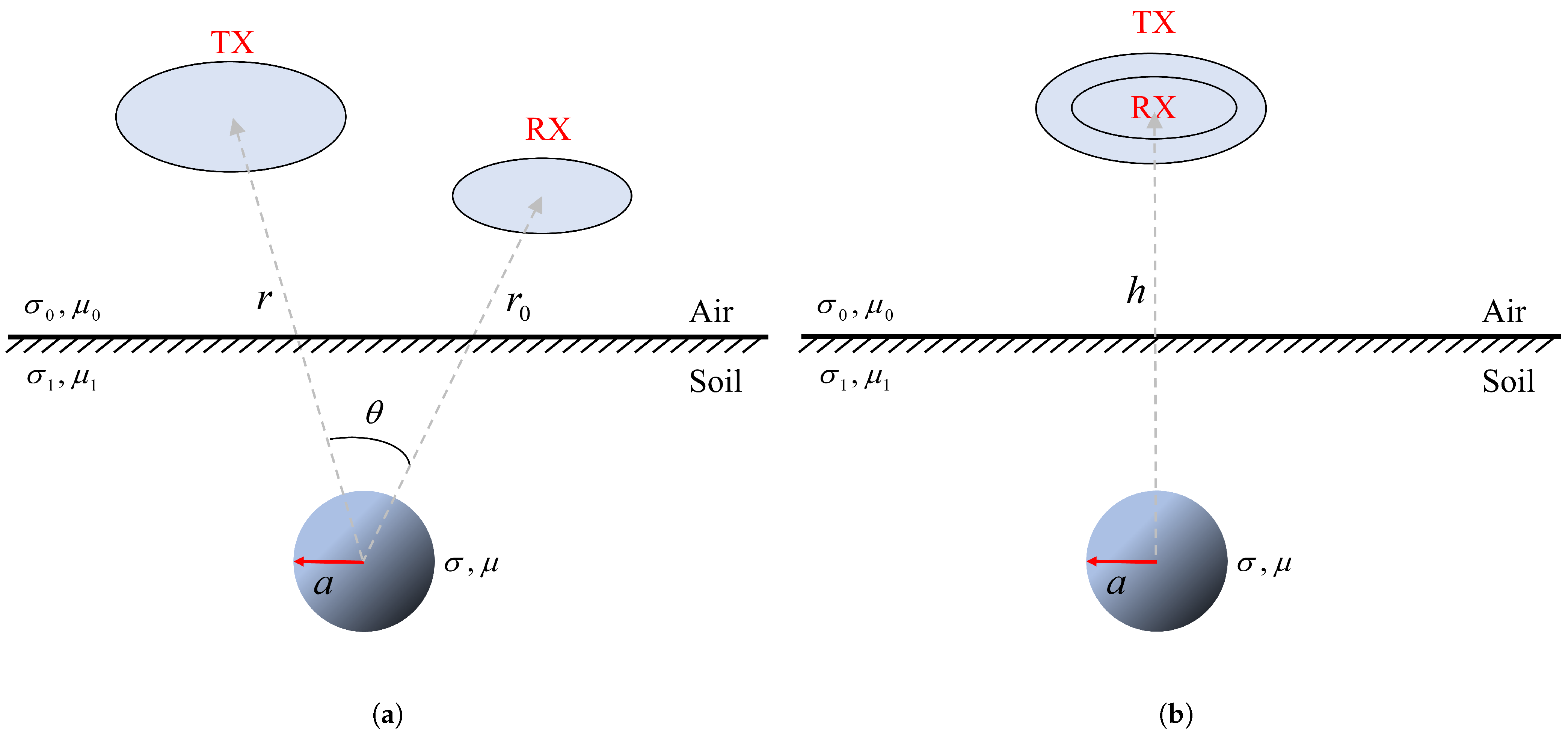
For a solid sphere, Grant and West gave an analytical expression of its electromagnetic response in a vertical magnetic dipole field [40]. The response model is shown in Figure 1a. $\sigma$ and $\mu$ are the conductivity and permeability of the solid sphere, respectively, ${\mu }_r=\mu /{\mu }_0$ is the relative permeability, and a is the radius of the sphere. TX is the transmitting coil, $\omega$ is the transmitting angular frequency, and $r_0$ is the radial distance between TX and the conductor sphere. RX is the receiving coil, and r is the radial distance between TX and the conductor sphere. $\theta$ is the vector angle between r and $r_0$. Therefore, the induced secondary magnetic field $H_{sz}$ in the z-axis at the receiving coil can be written as:

$$H_{sz}=\left(H_{r,r}+H_{\theta ,r}\right)cos{\theta }_r-\left(H_{r,\theta }+H_{\theta ,\theta }\right)sin{\theta }_r$$

(1)

where $H_{i,j}(i,j=r,\theta )$ represents j components of the secondary field from the i dipole source. The specific expression is as follows:

$$H_{r,r}=-\frac{m_r}{4\pi }\sum _{n=1}^{\infty }\left(X_n+i{Y}_n\right)\frac{a^{2n+1}}{{\left(r{r}_0\right)}^{n+2}}n(n+1)P_n(cos\theta )$$

(2)

$$H_{r,\theta }=-\frac{m_r}{4\pi }\sum _{n=1}^{\infty }\left(X_n+i{Y}_n\right)\frac{a^{2n+1}}{{\left(r{r}_0\right)}^{n+2}}n{P}_n^1(cos\theta )$$

(3)

$$H_{\theta ,r}=\frac{m_{\theta }}{4\pi }\sum _{n=1}^{\infty }\left(X_n+i{Y}_n\right)\frac{a^{2n+1}}{{\left(r{r}_0\right)}^{n+2}}n{P}_n^1(cos\theta )$$

(4)

$$H_{\theta ,\theta }=-\frac{m_{\theta }}{4\pi }\sum _{n=1}^{\infty }\left(X_n+i{Y}_n\right)\frac{a^{2n+1}}{{\left(r{r}_0\right)}^{n+2}}\times \left[n^2{P}_n(cos\theta )-\frac{n}{n+1}cot\left(\theta \right)P_n^1(cos\theta )\right]$$

(5)

where $m_r$ and $m_{\theta }$ represent the radial dipole moment and transverse dipole moment, respectively, $P_n$ is the n-th order Legendre polynomial, and $P_n^1$ is the associated Legendre polynomial.

The complex expression $X_n+i{Y}_n$ in Formulas (2)–(5) is called the response function, and contains the electromagnetic properties and size of the sphere. Other terms in the formula are all real, and are only determined by the relative position between the sphere, the transmitter, and the receiver. The real part X of the response function is the in-phase response, and the imaginary part Y is the quadrature response. For a solid, permeable, and conductive sphere, the response function can be expressed as:

$$X_n+i{Y}_n=\frac{\left[\frac{1}{2}-{\mu }_r(n+1)\right]I_{n+1/2}\left(ka\right)+ka{I}_{n+1/2}^{\prime }\left(ka\right)}{\left[\frac{1}{2}+n{\mu }_r\right]I_{n+1/2}\left(ka\right)+ka{I}_{n+1/2}^{\prime }\left(ka\right)}$$

(6)

where $k^2=i\omega \mu \sigma$, $I_{n+1/2}\left(ka\right)$ is the modified spherical Bessel function of the first kind.

When the transmitting coil TX is concentric with the receiving coil Rx, as shown in Figure 1b, the response function is simplified as:

$$X+iY=\frac{\left[{\mu }_0\left(1+k^2{a}^2\right)+2{\mu }_r{\mu }_0\right]sinh\left(ka\right)-\left(2{\mu }_r{\mu }_0+{\mu }_0\right)kacosh\left(ka\right)}{\left[{\mu }_0\left(1+k^2{a}^2\right)-{\mu }_r{\mu }_0\right]sinh\left(ka\right)+\left({\mu }_r{\mu }_0-{\mu }_0\right)kacosh\left(ka\right)}$$

(7)

where sinh and cosh are hyperbolic sine and hyperbolic cosine functions, respectively.

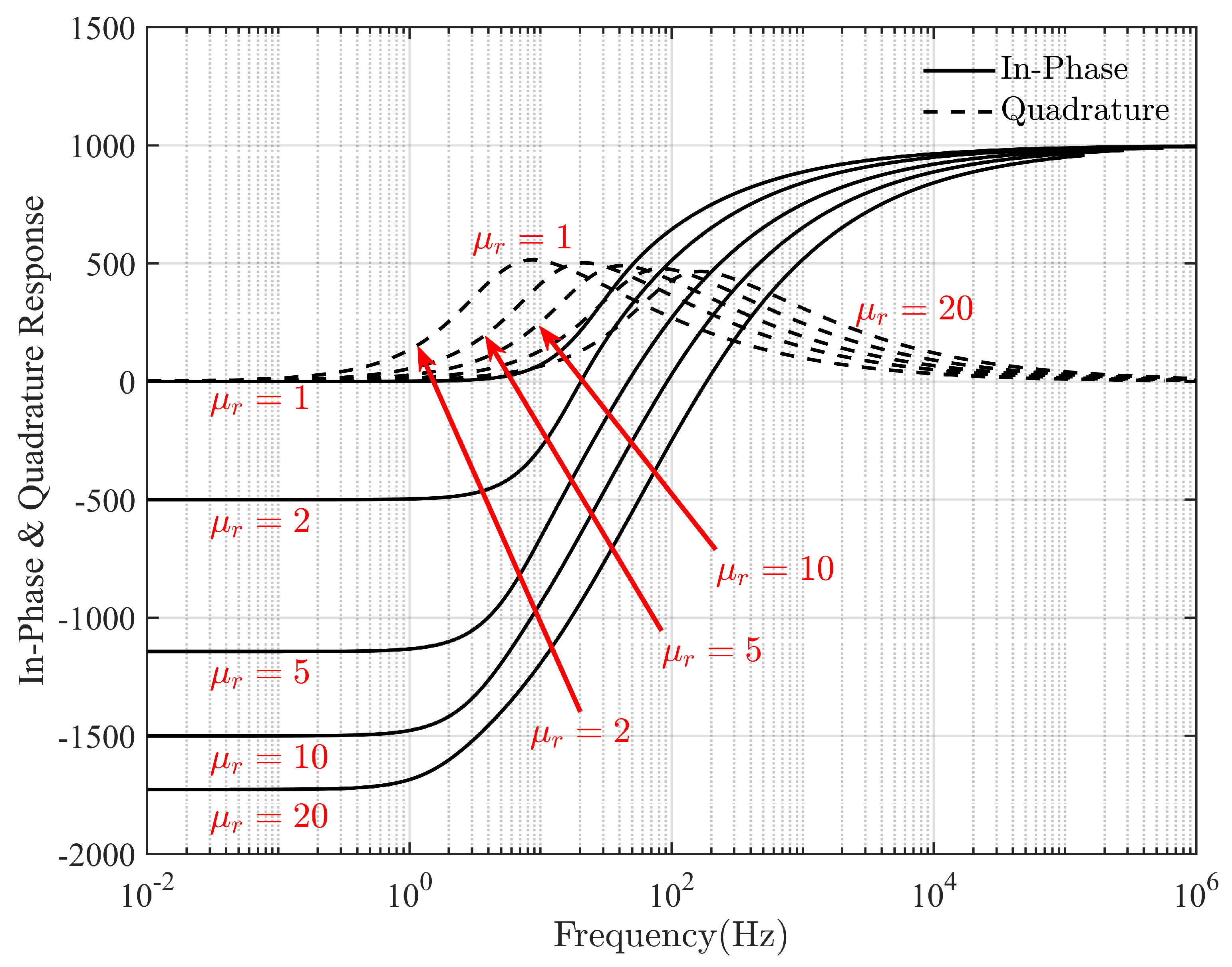
Then, the secondary field $H_s$ is normalized against the primary field $H_p$ and multiplied by ${10}^6$, with part-per-million (ppm) as the unit. Figure 2 shows the frequency domain response of the sphere with different relative permeabilities.

$$ppm=\frac{H_s}{H_p}\times {10}^6$$

(8)

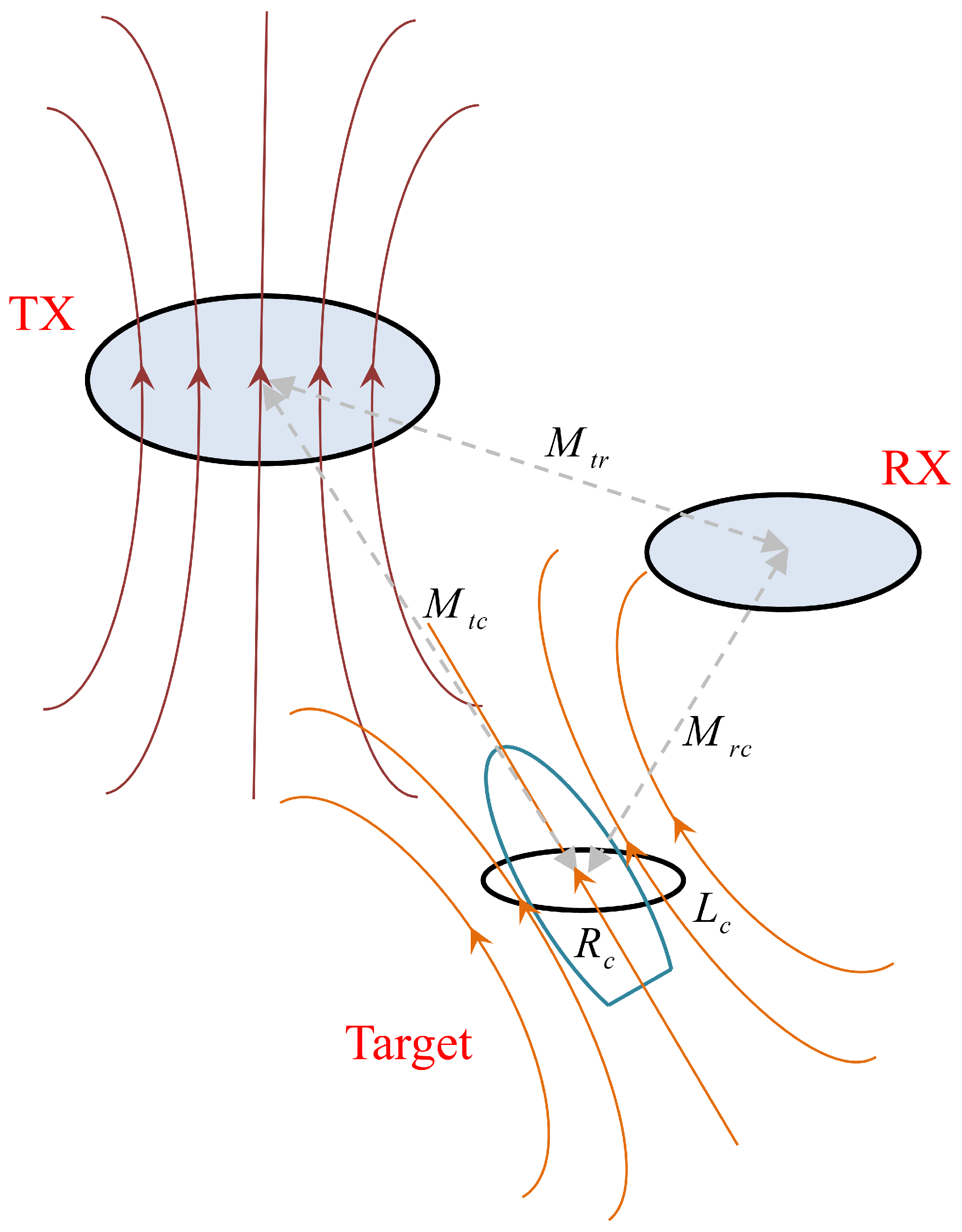
At present, only the solid sphere has an analytical solution of the frequency domain electromagnetic response. For general shape targets, the response can be equivalent to that of a standard coil with inductance and resistance, and the principle can be described by the coupling relationship between three inductance coils [40]. As shown in Figure 3, TX is the transmitting coil, RX is the receiving coil, and the target can be equivalent to the inductive coil with resistance $R_c$ and inductance $L_c$. $M_{tc},M_{rc}$, and $M_{tr}$ are the mutual inductance between TX and the target, RX and the target, and TX and RX, respectively. The secondary field signal ${\epsilon }_{H_s}$ relative to the primary field signal ${\epsilon }_{H_p}$ can be written as follows:

$$\frac{{\epsilon }_{H_s}}{{\epsilon }_{H_p}}=-\frac{M_{tc}{M}_{rc}}{M_{tr}{L}_c}\frac{{\alpha }^2+j\alpha }{1+{\alpha }^2}=-\frac{M_{tc}{M}_{rc}}{M_{tr}}\frac{{\omega }^2{L}_c+j\omega R_c}{{\omega }^2{L}_c^2+R_c^2}$$

(9)

where $\alpha =\omega L_c/R_c$.

It can be noted that the front part of the formula $-M_{tc}{M}_{rc}/M_{tr}{L}_c$ only depends on the relative position and size of the three coils, and the remaining term is a complex function $f\left(\alpha \right)=\left({\alpha }^2+j\alpha \right)/\left(1+{\alpha }^2\right)$ of the dimensionless variable $\alpha$. $\alpha$ depends on the frequency of the electromagnetic field and the electrical characteristics of the standard coil. For the variable $\alpha$, there are three trends:

(1)

When $\alpha \to 0$, ${lim}_{\alpha \to 0}f\left(\alpha \right)=j\alpha$, the response value is dominated by the quadrature component, and the phase difference between the secondary field and the primary field is approximately 90${}^{\circ }$.

(2)

When $\alpha \to \infty$, ${lim}_{\alpha \to \infty }f\left(\alpha \right)=1$, the response is purely in-phase, without a quadrature component, and the phase difference between the secondary field and the primary field is approximately 180${}^{\circ }$.

(3)

When $\alpha =1$ , the amplitudes of the in-phase response and the quadrature response are equal.

The in-phase component and quadrature component are:

$$Re\left(\frac{{\epsilon }_{H_s}}{{\epsilon }_{H_p}}\right)=-\frac{M_{tc}{M}_{rc}}{M_{tr}{L}_c}\frac{{\alpha }^2}{1+{\alpha }^2}=-\frac{M_{tc}{M}_{rc}}{M_{tr}}\frac{{\omega }^2{L}_c}{{\omega }^2{L}_c^2+R_c^2}$$

(10)

$$Im\left(\frac{{\epsilon }_{H_s}}{{\epsilon }_{H_p}}\right)=-\frac{M_{tc}{M}_{rc}}{M_{tr}{L}_c}\frac{\alpha }{1+{\alpha }^2}=-\frac{M_{tc}{M}_{rc}}{M_{tr}}\frac{\omega R_c}{{\omega }^2{L}_c^2+R_c^2}$$

(11)

It is generally considered that the electromagnetic induction caused by abnormal targets is a linear system, so the induced secondary field signal has the same frequency as the primary field signal. In practical applications, multi-frequency signals are usually transmitted at the same time. Assuming that the frequency of the transmitted signal is ${\omega }_s={\omega }_1+{\omega }_2+{\omega }_3+\cdots =2\pi \left(f_1+f_2+f_3+\cdots \right)$, we express the induced secondary field and the transmitted primary field of a single frequency as $a_{2}sin\left({\omega }_{1}t+{\phi }_2\right)$ and $a_{1}sin\left({\omega }_{1}t+{\phi }_1\right)$. Then, the received signal is convolved with the standard sine and standard cosine signal of each frequency, respectively, which is equivalent to matching filtering the secondary field signal. This method can not only analyze the in-phase $\left(I\right)$ and quadrature $\left(Q\right)$ components of each secondary field from the multi-frequency received signal but can also eliminate the clutter and improve the signal-to-noise ratio. Taking ppm as the unit of the I and Q components, we can obtain the following formula:

$$I_{ppm}={10}^6·\frac{a_2}{a_1}cos\left({\phi }_1-{\phi }_2\right)$$

(12)

$$Q_{ppm}={10}^6·\frac{a_2}{a_1}sin\left({\phi }_1-{\phi }_2\right)$$

(13)

where $I_{ppm}$ and $Q_{ppm}$ are the real and imaginary parts of the abnormal response, respectively. It can be seen from Formulas (12) and (13) that the abnormal response only depends on the amplitude and phase relationship between the secondary field and the primary field.

3. System Design

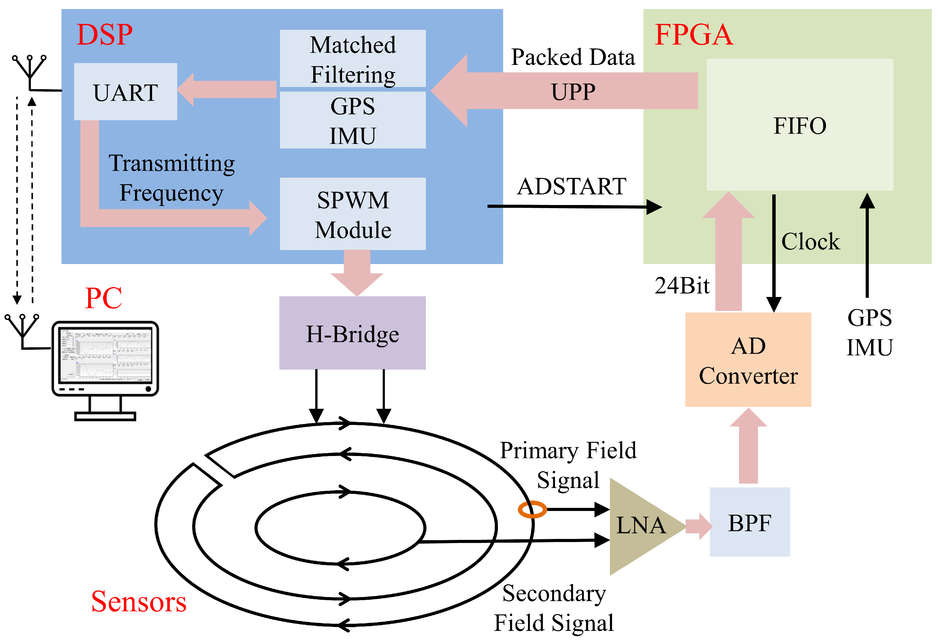
The AFEM-3 system mainly includes a sensor head, transmitting module, receiving module, and system control module. The system structure diagram is shown in Figure 4.

3.1. Sensor Head

The key to target detection using the frequency domain electromagnetic method lies in how to extract the weak induced secondary field signal for analysis and processing in the presence of a strong transmission magnetic field. The traditional HCP architecture sensor uses a group of transmitting, reference, and receiving coils to be placed separately on the same horizontal plane. The induction signal in the receiving coil is compensated by the induction signal in the reference coil to eliminate the primary field. However, it is difficult for this structure to completely eliminate the primary field signal, and the secondary field signal may be interfered with or even submerged, so the detection sensitivity is poor. In addition, because of its separated sensor structure, the spatial resolution of the detection is low.

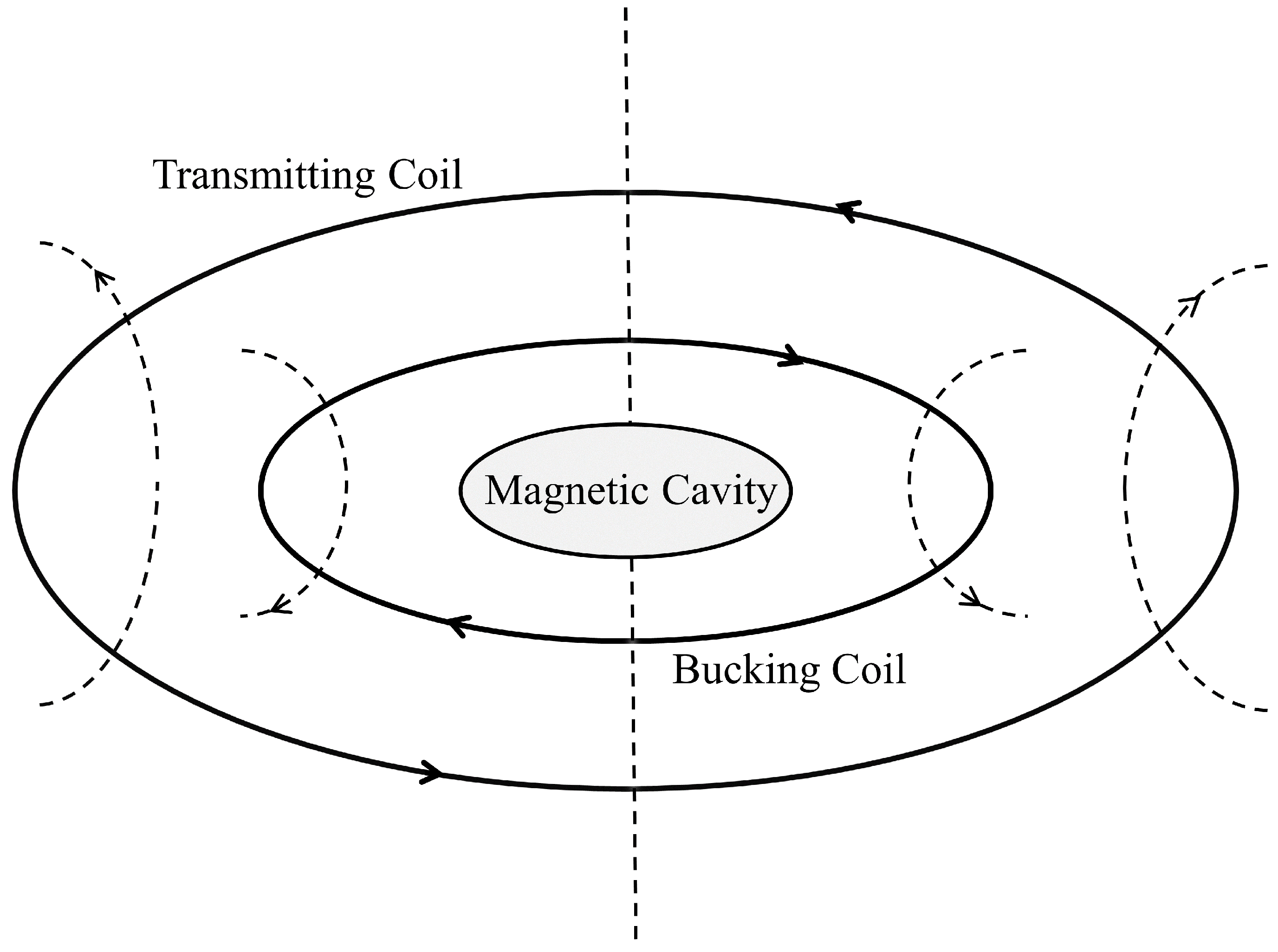
Therefore, we adopted a monostatic concentric coil sensor structure [41], as shown in Figure 5, using two coils with different radii and turns to be placed concentrically and connected in reverse series as the transmitting coil. After the alternating current is applied, the magnetic fields generated inside the two coils are in opposite directions, so a magnetic cavity with a magnetic flux close to zero will be generated at its central fixed position. Placing a receiving coil with a suitable radius at this position can effectively shield the influence of the primary field. Therefore, a sensor with high sensitivity can be placed near a strong dipole field to detect the weak secondary field signal excited by the subsurface target. This structure will have a high detection sensitivity and spatial resolution.

The quantitative calculation method of the sensor parameters is given below. First, by analyzing the characteristics of the magnetic field generated by a single circular coil, we can obtain:

$$B_z\left(r\right)=\frac{{\mu }_{0}I}{2a}\left[1+{\left(\frac{1}{2}\right)}^{2}3{\left(\frac{r}{a}\right)}^2+{\left(\frac{1·3}{2·4}\right)}^{2}5{\left(\frac{r}{a}\right)}^4+{\left(\frac{1·3·5}{2·4·6}\right)}^{2}7{\left(\frac{r}{a}\right)}^6+\dots \right]r\le a$$

(14)

where a is the radius of a single coil, I is the current, and r is the distance from a point on the coil plane to the center. The magnitude of the magnetic field is also normalized to ${\mu }_{0}I/2a$ at $r=0$, the loop center. The magnetic field intensity in the center of the loop is high, but the change rate of the magnetic field intensity along the radial direction of the loop plane is very small, so the magnetic field intensity is stable in space. Therefore, this spatial stability enables us to generate an opposite magnetic field by superimposing a concentric loop to generate an area with zero magnetic flux in the center.

Therefore, the basic relationship between the radius r of the receiving coil and the transmitting coil radius $R_1$, turns $n_1$, and the bucking coil radius $R_2$, turns $n_2$ can be deduced as follows:

$$\begin{array}{c}\frac{n_1}{R_1}\left[\frac{1}{2}+{\left(\frac{1}{2}\right)}^2\frac{3}{4}{\left(\frac{r}{R_1}\right)}^2+{\left(\frac{1·3}{2·4}\right)}^2\frac{5}{6}{\left(\frac{r}{R_1}\right)}^4+{\left(\frac{1·3·5}{2·4·6}\right)}^2\frac{7}{8}{\left(\frac{r}{R_1}\right)}^6+\dots \right]\hfill \\ =\frac{n_2}{R_2}\left[\frac{1}{2}+{\left(\frac{1}{2}\right)}^2\frac{3}{4}{\left(\frac{r}{R_2}\right)}^2+{\left(\frac{1·3}{2·4}\right)}^2\frac{5}{6}{\left(\frac{r}{R_2}\right)}^4+{\left(\frac{1·3·5}{2·4·6}\right)}^2\frac{7}{8}{\left(\frac{r}{R_2}\right)}^6+\dots \right]\hfill \end{array}$$

(15)

The transmitting coil, having a larger radius and more turns, is to be the principal transmitter of an active magnetic field, and the bucking coil generates the magnetic field in the opposite direction, which reduces the amplitude of the dipole field. The amplitude loss value is calculated by the following formula:

$$\mathrm{Amplitude}\mathrm{Loss}=\frac{n_2}{n_1}{\left(\frac{R_2}{R_1}\right)}^2$$

(16)

According to Formula (15), we designed a group of coils; the parameters are shown in

Table 1. Parameters of the coils.

Type	Radius (m)	Turns	Amplitude Loss
Transmitting Coil	0.4	9	5.35%
Bucking Coil	0.16	3
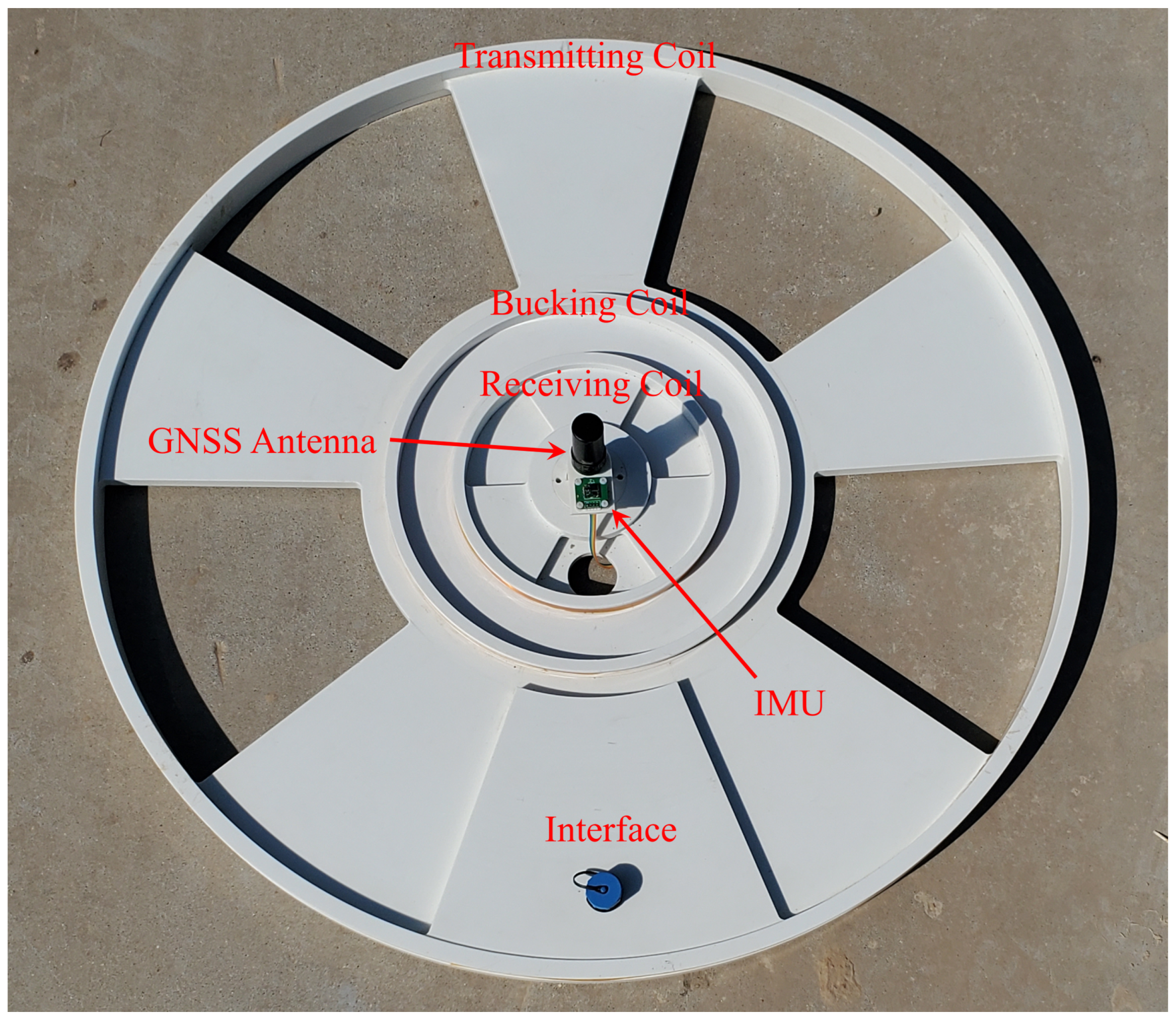
Receiving Coil	0.1065	100

. All three coils are hollow coils wound on the nylon skeleton with enamelled wires, and their resonant frequencies are far higher than the system bandwidth in order to avoid signal distortion caused by resonance. The nylon skeleton has the physical characteristics of a light weight, high dimensional stability, and difficult deformation. As a pod, it will not affect the balance of the UAV due to its weight, nor will it cause its internal shaking due to the movement of the UAV, so the overall sensor can maintain a good stability. In addition, GNSS and IMU modules were installed in the sensor center to measure the position and attitude of the sensor. The manufactured sensor is shown in Figure 6.

3.2. Transmitting Module

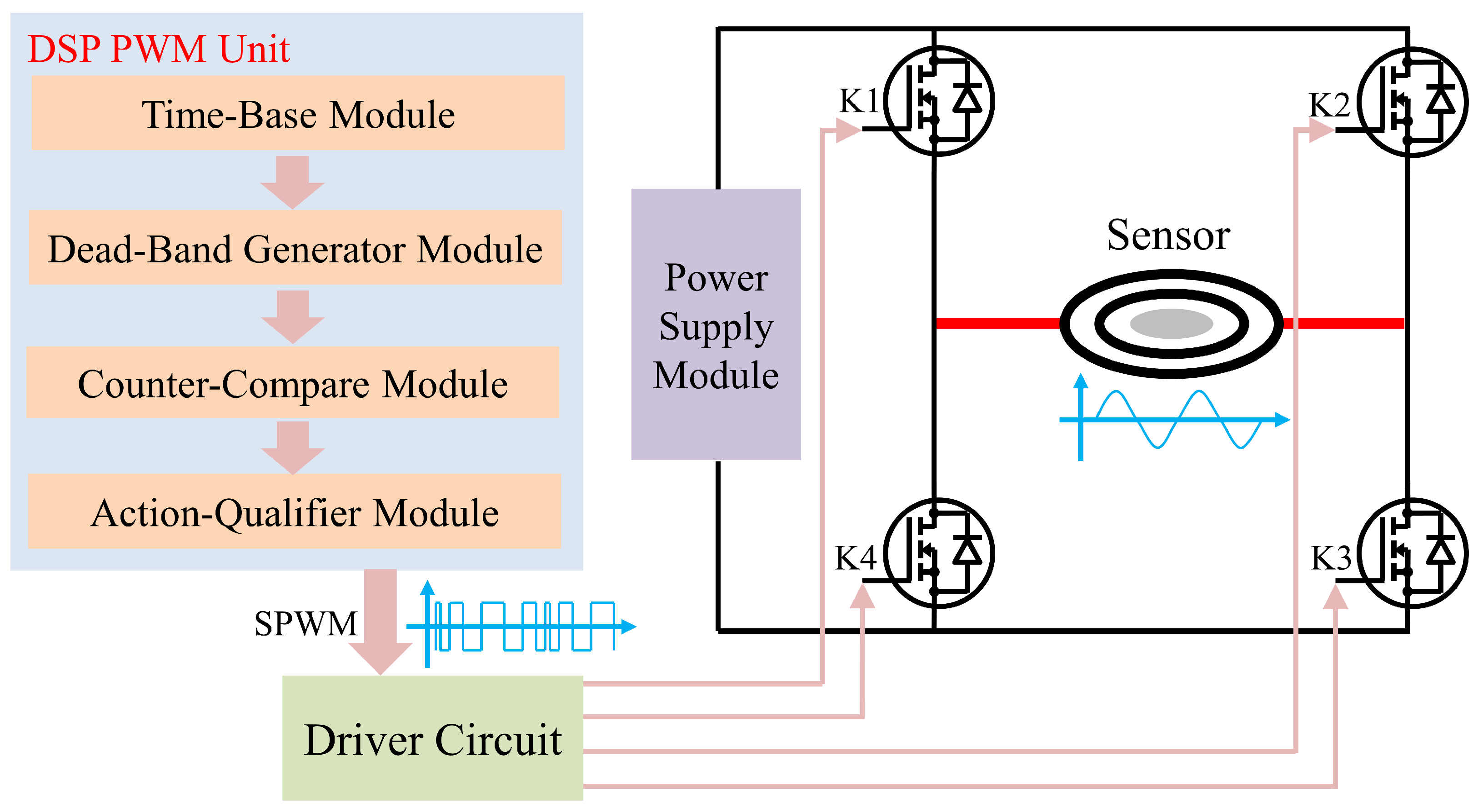
Figure 7 shows the structure diagram of the transmitting module, which is mainly composed of a DSP control unit, power drive circuit, H-bridge inverter circuit, and load coil. The transmitting module is mainly based on unipolar frequency multiplication SPWM modulation technology and H-bridge inverter technology. The SPWM signal is a PWM switching signal whose pulse width varies with sine [42,43]. Compared with the commonly used bipolar SPWM modulation technology, the unipolar frequency multiplication SPWM has two state transitions in a single carrier cycle, which is equivalent to doubling its carrier frequency. Therefore, it only contains (2n + 1)-th harmonics, and has smaller harmonic contents when the amplitude of the modulated wave is constant.

Because the SPWM signal is suitable for digital circuit generation, and has the advantages of an arbitrary frequency combination, low harmonic output and high precision, the control unit based on DSP generates the required SPWM switching signal. Then, the driving circuit controls the opening and closing of the four MOSFET gates on the H-bridge. Due to the inductive reactance of the load coil, the current cannot occur a sudden change, so it converts the direct current into the alternating current with the required frequency.

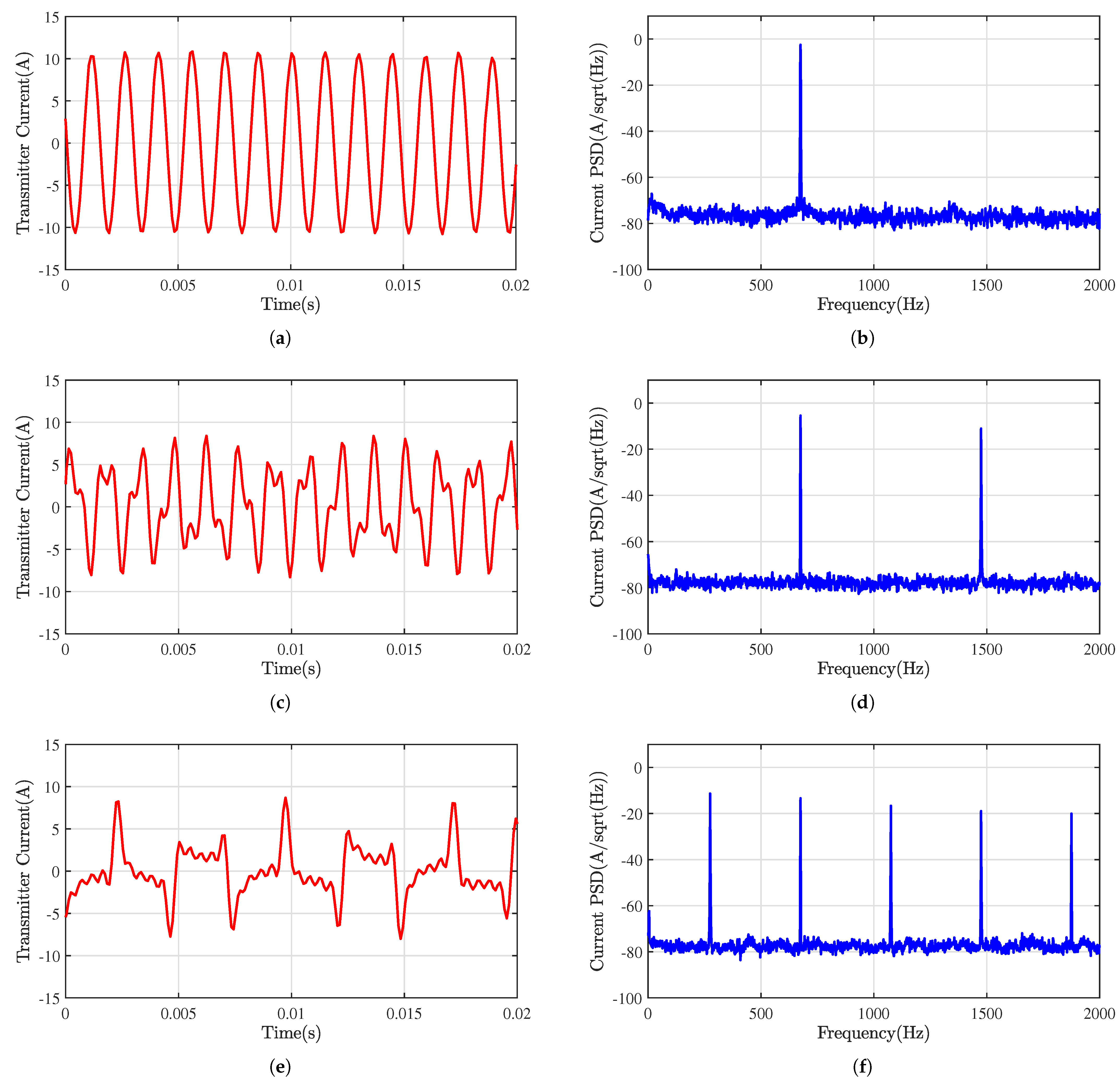
In order to minimize the power line noise, half of the power line frequency is usually used as the basic frequency of signal transmission. In Asia, Europe, Africa, and other regions where the power line frequency is 50 Hz, the transmitting frequency is an odd multiple of 25 Hz. Similarly, in America and other regions where the power line frequency is 60 Hz, an odd multiple of 30 Hz is used.

Figure 8 shows the waveform and power spectrum of transmitting a current of a single-frequency, dual-frequency, and five-frequency combination. It can be seen from the figure that, when transmitting a single frequency of 675 Hz, the peak current is approximately 10.6 A, and the signal-to-noise ratio is approximately 75 dB. The equivalent transmitting magnetic moment of the sensor designed in Section 3.1 is approximately 45.4 A$·{\mathrm{m}}^2$. Affected by the coil inductive reactance, the higher the transmitting frequency, the smaller the amplitude of the transmitting current.

3.3. Receiving Module

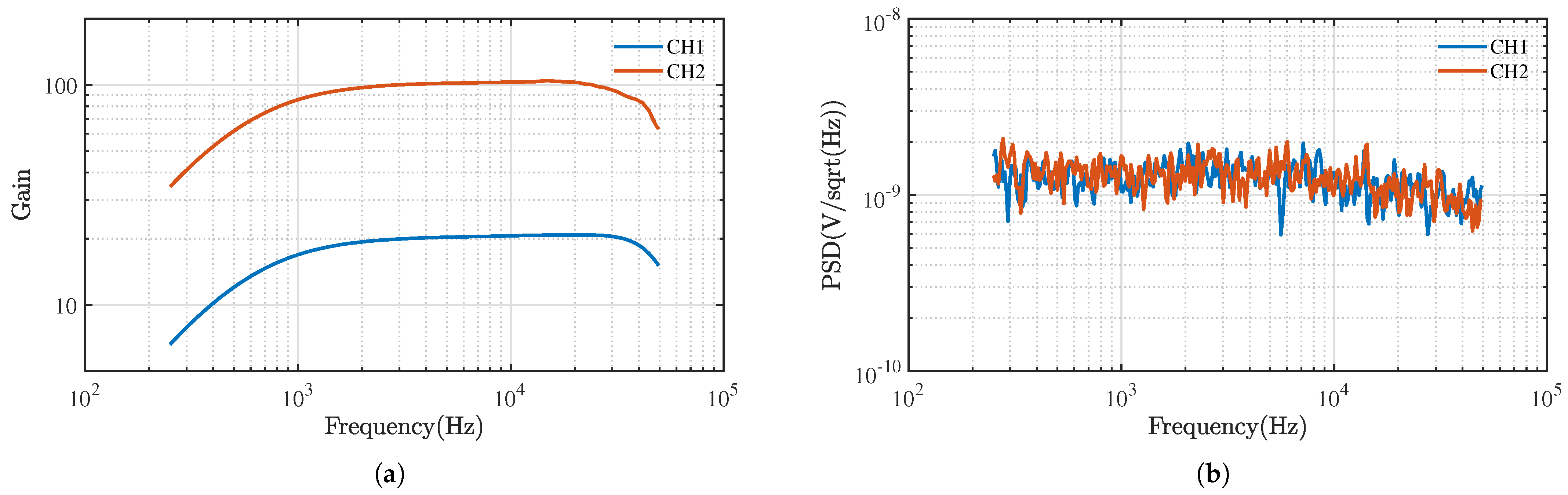
The receiving module is mainly composed of an analog signal processing part and an analog-to-digital conversion part. First, the original signal is amplified by the low-noise amplifier (LNA). Then, the clutter signal interference outside the available frequency band is filtered through an active band-pass filter based on Sallen–Key topology. Finally, the single-ended signal is converted into a differential signal. There are two receiving channels: one channel collects the transmitting current through the hall current sensor, and the other channel receives the induced voltage signal of the receiving coil. The performance of the analog signal conditioning module is shown in Figure 9. The two channels amplify the original signals by 20 times and 100 times, respectively, and the noise power density of the equivalent input is approximately 1.53 $\mathrm{nv}\sqrt{\mathrm{Hz}}$. Finally, the signal is digitized by a 24-bit Sigma-Delta ADC.

3.4. System Control Module

The system control module consists of DSP and field programmable gate array (FPGA) dual processors. The FPGA controls the serial port to collect GNSS and IMU data, in which, the GNSS module adopts a full-band positioning signal, and, through the real-time kinematic (RTK) technology, can realize the accurate positioning of the sensor head with centimeter-level accuracy. In addition, FPGA mainly provides a time sequence for the ADC and drives it to collect data at a sampling frequency of 78.125 kHz, with a single sampling of 1/12.5 s and 6250 data points. A single set of data collected by FPGA is received through the DSP universal parallel port interface. The standard sine and cosine signals of the transmitted frequencies are preset in DSP, and the in-phase and quadrature response of each frequency can be calculated efficiently by its multiple functional unit. The DSP communicates with the host computer through the serial port, which can receive the instructions of the host computer, and, at the same time, send the in-phase and quadrature response, position, and attitude data to the host computer in real-time for display and storage.

3.5. UAV Platform

The performance of the UAV platform has a crucial influence on the detection results. In order to meet the application scenarios that the system can detect in complex environments, we chose the multi-rotor UAV instead of the fixed-wing UAV because it can fly more stably and fly at low altitudes and low speeds. In addition, it is necessary to focus on the maximum load weight, endurance time, and flight accuracy of the multi-rotor UAV. In terms of the maximum load weight, we measured the total weight of our whole detection system (including sensors, system chassis, batteries, and cables) as being approximately 10.1 Kg. To improve the detection accuracy, it is necessary to improve the flight accuracy of the UAV and make the flight path spacing smaller. Therefore, it is necessary to choose a UAV that supports the RTK technology and supports the flight path planning with smaller spacing. Moreover, the UAV platform with a terrain-following function should be selected to ensure flight safety when conducting experiments in complex terrain areas.

After investigating many UAVs made in China, there are three more suitable UAV platforms, whose key parameters are shown in

Table 2. Comparison of the UAV parameters.

Company	Model	Maximum Load	Minimum Route Interval	Endurance	Terrain Following	RTK
Sunward	SUMP3206	13 Kg	0.4 m	⩾40 min (6.5 Kg load)	Support	Support
Lyncon	S1600	9 Kg	0.5 m	⩾30 min (6 Kg load)	No Support	Support
DJI	MG1P	10 Kg	3 m	⩾9 min (10 Kg load)	Support	Support

. By comparing their parameters and conducting relevant tests, we finally chose the SUMP3206 UAV platform manufactured by Hunan Zhuzhou Sunward Technology Co., Ltd., China. This UAV platform supports route planning, and its flight parameters can be freely configured according to requirements. Once the flight mission is planned in the software, and the UAV can automatically execute the mission without human participation.

4. Experimental Results

To test the performance of AEFM-3 system, we designed static and field experiments for the system. In the static experiment, we set multiple sensor positions, and each measurement kept the sensor and target positions unchanged, collecting data for approximately 5 s. Then, the sensor position was changed to collect data repeatedly. Finally, the experimental results were compared with the simulation results. In the field experiment, the UAV was used to carry the detection system to scan and detect the survey area. The system can record the position and electromagnetic response in real-time, and the response map of the survey area can be obtained after interpolating the data.

4.1. Static Experiment

In order to verify the consistency between the actual measured response of the frequency domain system and the theoretical model, we carried out static experiments using standard coils. The standard coil is wound by copper wire, with a radius of 8.5 cm, an inductance of 1.903 mH, and a resistance of 977.766 m$\Omega$. Firstly, the center position of the standard coil was fixed as the coordinate zero point, and the sensor plane was set to be parallel to the standard coil plane. Then, the sensor was made to move along a straight line in the range of −1 m∼1 m at the height of H above the standard coil. Finally, the simulation and practical experiments were carried out under this experimental configuration.

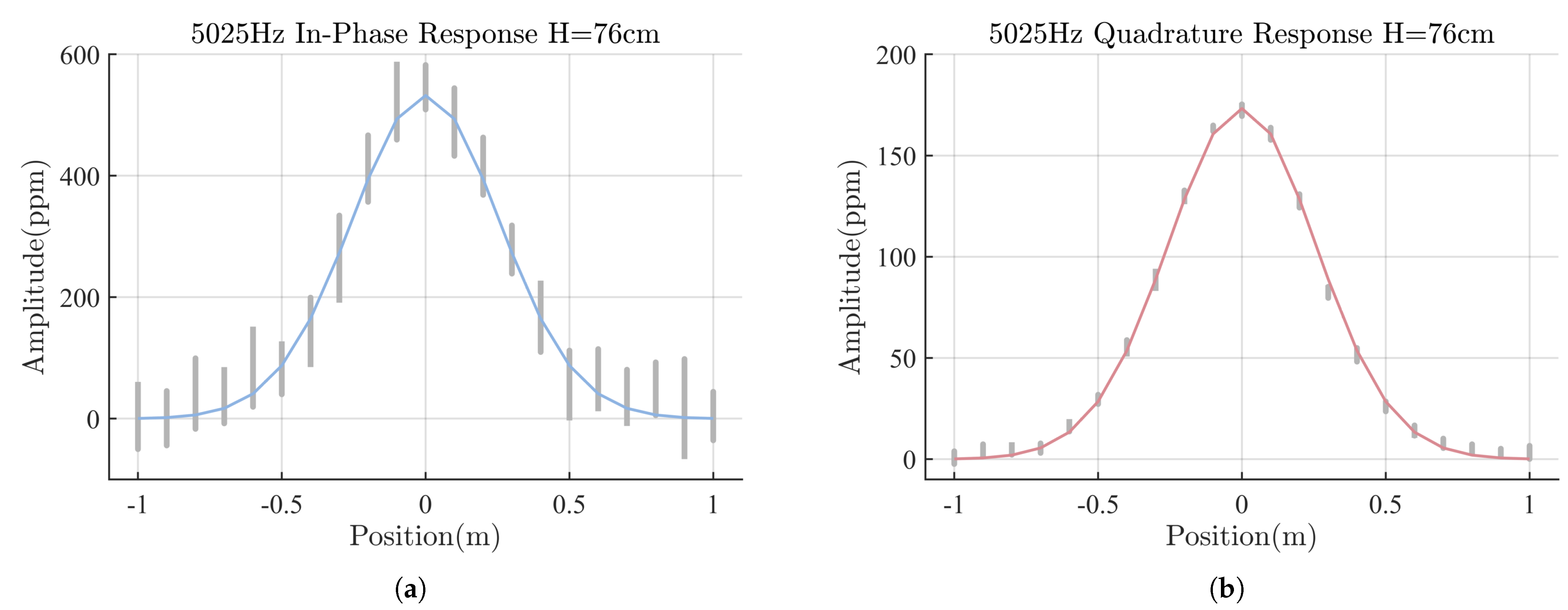
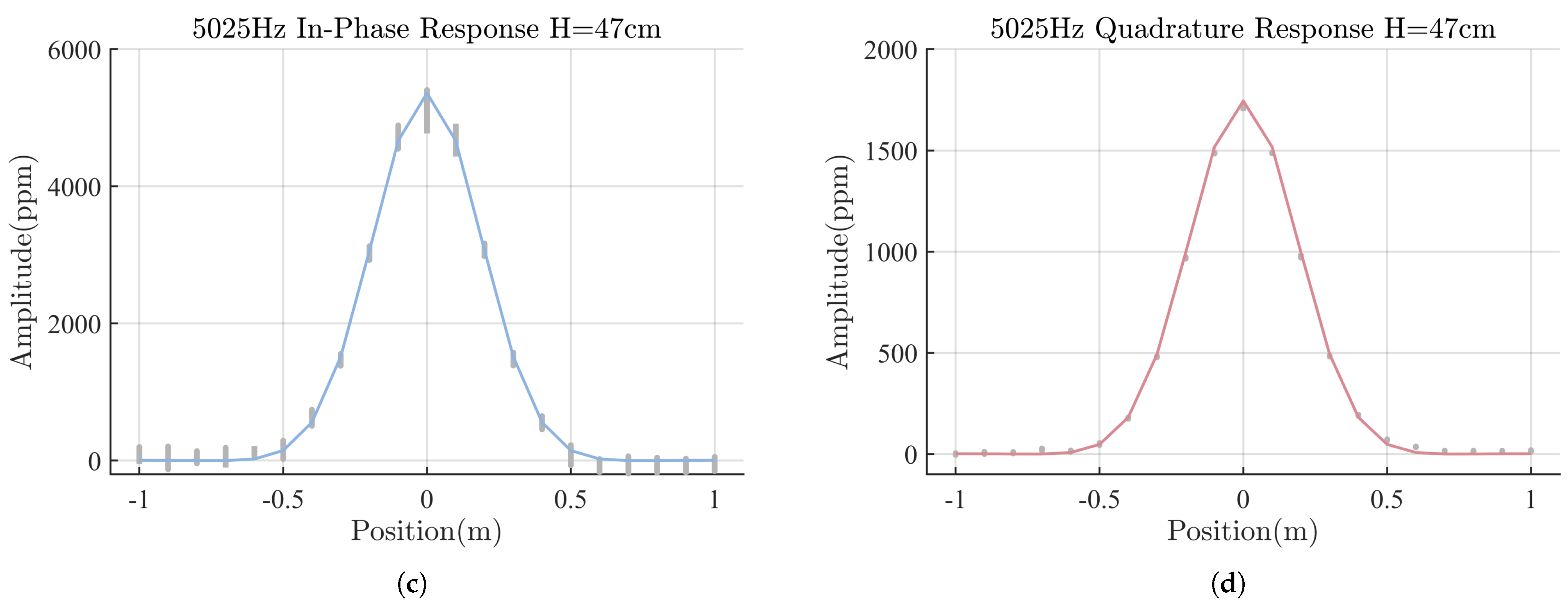
According to Formulas (10) and (11) in Section 2, the transmission frequency was set as 5025 Hz, and the height H was taken as 0.47 m and 0.76 m, respectively. The response value generated by the standard coil when the sensor moves in the range of −1 m∼1 m along the survey line was calculated, as shown by the curve lines in Figure 10. It can be seen from the figure that, since the sensor is of a concentric coil structure, there will be an obvious single-peak abnormal response when it moves right above the standard coil. The height H affects the response amplitude and the response change rate along the survey line. The higher the height, the smaller the response amplitude and the smaller the change rate.

In addition, we performed the actual measurement experiment on the standard coil by using the AFEM-3 system. On the premise of ensuring that the transmitting frequency and height H were consistent with the simulation experiment, 21 points were taken at intervals of 0.1 m in the range of −1 m∼1 m of the survey line, and the response of the standard coil was measured, respectively. The results are shown by the vertical lines in Figure 10. The entire measured response was processed by removing the direct current component, and the length of the vertical line represents the fluctuation range of the response. It can be seen from the figure that the quadrature response signal-to-noise ratio is obviously larger than that of the in-phase response. Because the coil is wound by copper wire, the relative permeability of copper is 1, while the in-phase response is mainly affected by relative permeability, and the quadrature response is mainly related to the conductivity. Moreover, at two different heights, the amplitude and change rate of the simulated response curve are basically consistent with the measured response, which verifies the correctness of the frequency domain system.

4.2. Field Experiment

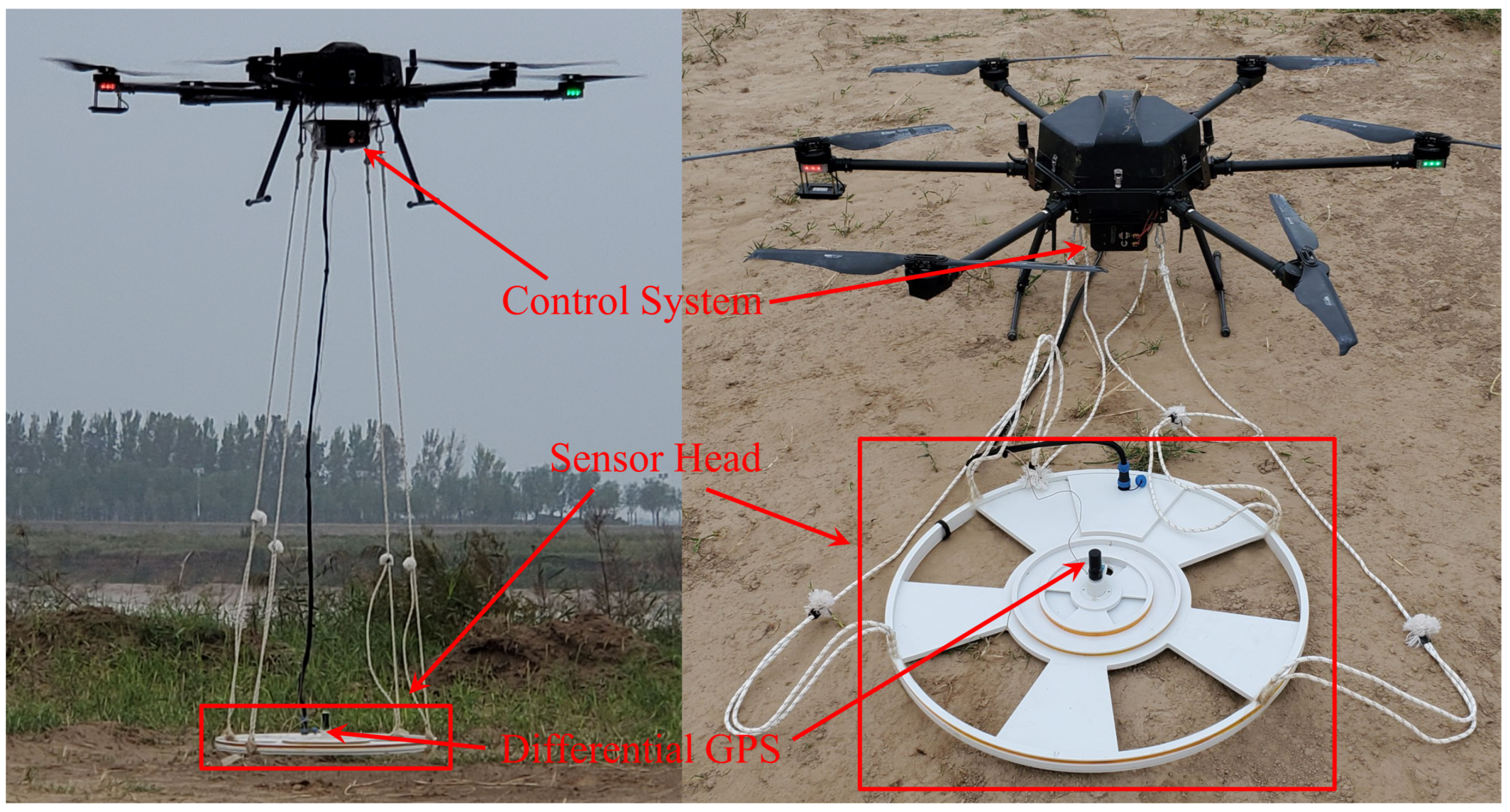
In order to test the ability of AFEM-3 system to detect small targets in the field, we conducted a field experiment in Huayin, Shaanxi Province, China. An open and flat test region was selected, whose size was approximately 6 m × 7 m. Eight metal targets with different shapes, sizes, and materials were placed in the test region. The parameters and positions of the targets are shown in

Table 3. Descriptions of targets used in the field experiment.

Target ID	Material	Attitude	Size (cm)	Position (m)	Horizontal Error (m) 1
$\star 1$	Steel	Horizontal	$\Phi$2 15.5 × 2	(1.65, 4.82, −0.20)	0.10
$\star 2$	Aluminum	Horizontal	20 × 20 × 0.5	(1.46, 3.15, −0.45)	0.12
$\star 3$	Steel	W-E 3 Horizontal	$\Phi$ 8 × 28	(1.62, 1.24, −0.40)	0.10
$\star 4$	Ferromagnetic	Vertical	$\Phi$ 15.5 × 25	(2.94, 3.29, −0.60)	0.13
$\star 5$	Ferromagnetic	Vertical	$\Phi$ 6 × 10	(3.34, 1.48, −0.25)	0.19
$\star 6$	Aluminum	Horizontal	25 × 18 × 12	(4.10, 5.07, −0.55)	0.17
$\star 7$	Ferromagnetic	SW-NE 4 Horizontal	$\Phi$ 10 × 20	(4.81, 3.48, −0.45)	0.18
$\star 8$	Steel	Vertical	$\Phi$ 6 × 18.5	(4.35, 2.00, −0.35)	0.14

¹ Horizontal error means the error between the measured value and the real value. ² Φ means outer diameter. ³ W-E means that the direction of head to tail is from west to east. ⁴ SW-NE means that the direction of head to tail is from southwest to northeast.

. Before the experiment, 12 survey lines with an interval of 0.5 m in the north–south direction were preprogrammed by the UAV, the AFEM-3 system was mounted on the UAV, and the flight altitude of the UAV was set to keep the sensor approximately 0.4 m from the ground. Once the flight trajectory was programmed, the UAV system was able to automatically perform the survey task so that the electromagnetic system could collect the electromagnetic response and position information along the survey line. The electromagnetic detection system based on a small six-rotor UAV platform is shown in Figure 11.

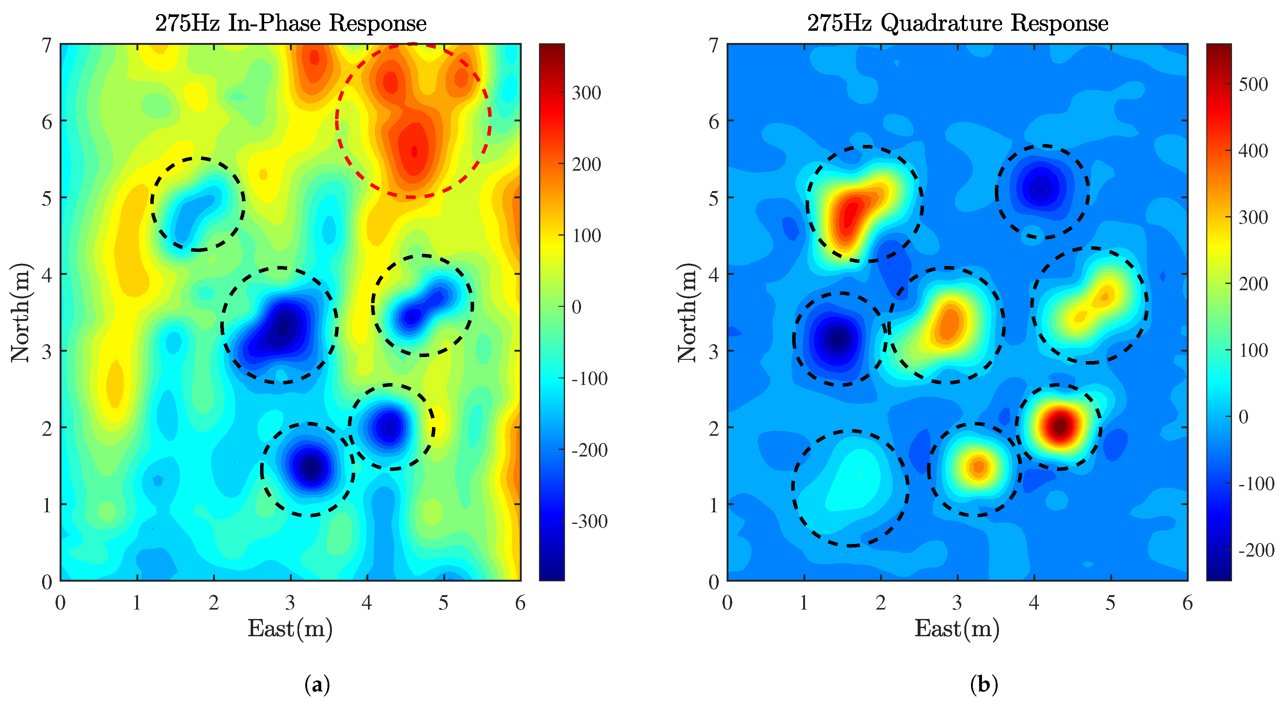
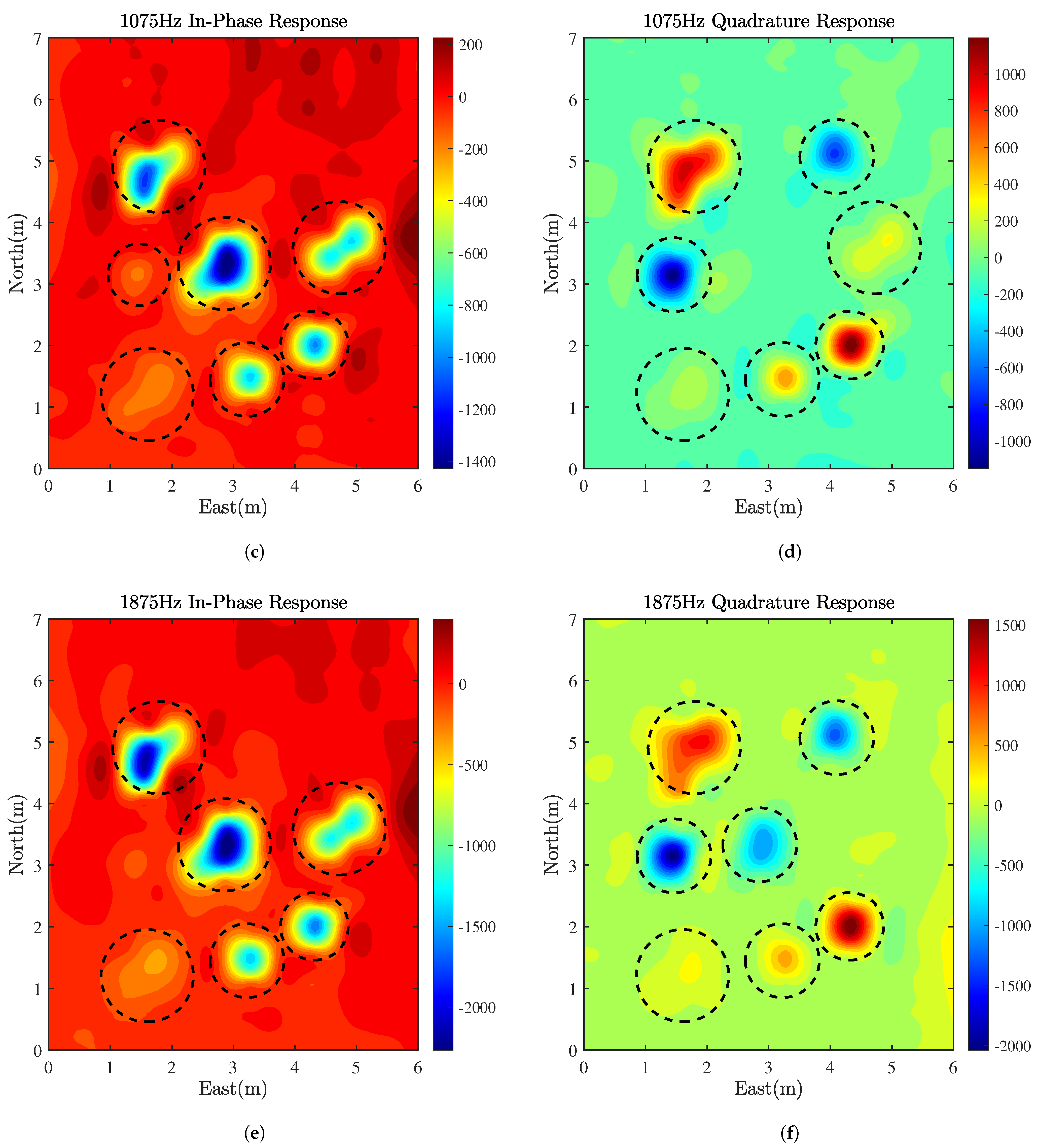
Three test frequencies of 275 Hz, 1075 Hz, and 1875 Hz were selected for the experiment. After the measurement, undesired data were cut off. The motion track of the sensor and the schematic of the target location are shown in Figure 12, where the size of the target in the figure does not represent the actual size of the target. We used the ’v4’ interpolation method built in Matlab to interpolate the data. This method is biharmonic spline interpolation with second-order continuity. The results obtained by this method are more suitable for this experiment, so the two-dimensional in-phase and quadrature response map of the survey at each frequency can be obtained, as shown in Figure 13.

In Figure 13, after visual inspection, we marked the maximum and minimum responses of the targets that can be clearly observed with black dotted circles. It can be seen from Figure 13b that all eight targets can be effectively detected. Except for the obvious false response at the red dotted circle in Figure 13a, the signal-to-noise ratio of other figures is high. The location of the target can be inverted by the peak value of the abnormal response, and, compared with the real location of the target, the positioning horizontal error can be obtained, which is given in Table 2. The errors are all within 20 cm.

It is worth noting that, regarding the quadrature response at the frequency of 275 Hz, as shown in Figure 13b, target $\star 2$ and target $\star 6$ have unique negative responses that are different from other targets. According to the known target materials, it can be concluded that target $\star 2$ and target $\star 6$ are made of aluminum, and other targets are mostly made of ferromagnetic or steel. The relative permeability of aluminum is 1, and the in-phase response is mainly affected by the relative permeability, so it is difficult to have an obvious abnormal response in Figure 13a,c,e This feature can help us to distinguish the materials of the targets.

Comparing the response of target $\star 4$ in Figure 13b,d,f, we found that the abnormal response is positive at 275 Hz, almost zero at 1075 Hz, and negative at 1875 Hz. It can be inferred that, in this frequency band, the quadrature response increases with the increase in frequency, approximately 1075 Hz is the zero point of the quadrature response of target $\star 4$, and, similarly, the zero point of target $\star 7$ is around 1875 Hz. The frequency of the target response zero point is also one of the characteristics of the target.

For ferromagnetic and steel targets, the intrinsic dipole intensity of the three axes is closely related to their shape. Generally, the intensity of the intrinsic dipole along the principal axis is the largest. Although target $\star 5$ and target $\star 8$ are small in size, they are placed in a vertical attitude, and their induced dipole intensity along the principal axis direction is the largest, which is consistent with the dipole direction of the sensor, so the response is more obvious. Because target $\star 3$ and target $\star 7$ are placed horizontally, the induced dipole intensity along the principal axis direction is perpendicular to the dipole direction of the sensor, and their depth is relatively deep. These comprehensive factors lead to a small response value.

In general, the AFEM-3 system can effectively detect all eight targets, and the target positioning errors are all within 20 cm. By comparing the results of multiple frequencies, the characteristics of the target can be analyzed and further used for target classification. However, there may also be some false responses. The reasons are as follows. First, there may be other metal impurities in the ground that cause interference. Then, the interference of the UAV platform and the shaking of the sensor during the measurement also may cause a deviation in the measurement data. Finally, the interpolation method will also affect the image quality.

5. Discussion

In this paper, a broadband frequency domain electromagnetic system AFEM-3 based on a UAV platform is proposed, and the design and technology of the system are introduced in detail from five parts: the sensor head, transmitting module, receiving module, system control module, and UAV platform. To the best of our knowledge, this is the first time that a small frequency domain electromagnetic system is integrated on a multi-rotor UAV platform for small target detection. After the experiment, the system can detect subsurface targets within 2 m.

5.1. Main Advantages

• The AFEM-3 system is based on the UAV platform. Compared with the traditional hand-held or vehicle-towed system, it can work more efficiently in some areas with a complex terrain or dangerous areas, such as desert, marsh, sea beach, shooting range, etc., while avoiding the danger caused by manual operation.
• Using unipolar frequency multiplication SPWM technology, the transmitting module can generate multi-frequency transmitting waveforms of arbitrary combinations of frequencies with low total harmonic distortion. Compared with the traditional bit-stream transmitting method, the SPWM technology does not depend on the load, so it is convenient to match different transmitting coils by using the same circuit and system.
• The sensor head integrates GNSS and IMU modules, which can collect position and attitude data at the same time in the measurement process, and the position measurement accuracy is centimeter-level. Based on the supporting PC software developed by us, all of the data can be observed and stored in real-time, and the two-dimensional response map of the survey area can be obtained quickly after the measurement is completed.

5.2. Limitations and Future Work

• At present, the sensor and the UAV system are in a soft connection state. When the experimental environment is harsh, especially when the wind speed is high, the suspended sensor will be affected by the wind; at the same time, the UAV flight state will also be affected by the wind, and its influence will be superimposed on the sensor again.
• When the geological environment noise is large—for example, the target to be measured is located in magnetic soil or there are many metal impurities in the underground environment—the method of separating the interested response from the complex environmental response is an ongoing challenge.
• The response characteristics of isolated targets are obvious. If multiple targets are close, the abnormal responses might be completely overlapping. If a big target and a small target are close, when the depth is the same, the response of the big target is usually dominant. When the depth of the big target is deep, the response of the small target will be dominant.

In future work, we will continue to improve the detection system. On the one hand, the hardware structure of the system needs to be optimized to reduce the measurement error caused by the platform. On the other hand, the algorithm is designed to process the signal, improve the signal-to-noise ratio, realize the automatic positioning of the target, further identify the magnetic moment, size, and shape of the target, and finally realize the classification of the target.

6. Conclusions

In this paper, a broadband frequency domain electromagnetic system AFEM-3 based on a small six-rotor UAV platform is presented, and its technology is introduced in detail from the system structure to data processing algorithm. The sensor head uses a concentric compensation sensor architecture and integrates GNSS and IMU modules. Based on the self-developed upper computer software, the target response, sensor attitude, and position information can be observed in real-time. Multi-frequency transmitting waveforms with low total harmonic distortion are generated based on unipolar frequency multiplication SPWM modulation technology. The collected data are processed and transmitted by DSP. Through the static experiment of the standard coil, the experimental results are consistent with the theoretical simulation results both in signal amplitude and trend, which verifies the correctness of the system. The field experiments show that the AFEM-3 system can effectively detect all eight metal targets with different sizes, materials, and shapes. Simple data processing can provide clear features and horizontal positions of the targets, and the positioning errors are all within 20 cm. Different targets have different sensitivities to different frequencies, which makes it possible to classify targets. The AFEM-3 system is easy to operate and highly automated, so it has great advantages in UXO detection, especially in some soft soil, swamps, and other areas that are difficult to enter manually.