Article

Measuring Understory Fire Effects from Space: Canopy Change in Response to Tropical Understory Fire and What This Means for Applications of GEDI to Tropical Forest Fire

1
Department of Ecology, Montana State University, Bozeman, MT 59715, USA
2
Departamento de Biología, Facultad de Ciencias, Universidad Nacional de Colombia, Bogotá 111321, Colombia
3
School of Informatics, Computing and Cyber Systems, Northern Arizona University, Flagstaff, AZ 86011, USA
*
Author to whom correspondence should be addressed.
Remote Sens. 2023, 15(3), 696; https://doi.org/10.3390/rs15030696
Submission received: 8 December 2022 / Revised: 16 January 2023 / Accepted: 23 January 2023 / Published: 24 January 2023

Abstract

:
The ability to measure the ecological effects of understory fire in the Amazon on a landscape scale remains a frontier in remote sensing. The Global Ecosystem Dynamics Investigation’s (GEDI) LiDAR data have been widely suggested as a critical new tool in this field. In this paper, we use the GEDI Simulator to quantify the nuanced effects of understory fire in the Amazon, and assess the ability of on-orbit GEDI data to do the same. While numerous ecological studies have used simulated GEDI data, on-orbit constraint may limit ecological inference. This is the first study that we are aware of that directly compares methods using simulated and on-orbit GEDI data. Simulated GEDI data showed that fire effects varied nonlinearly through the canopy and then moved upward with time since burn. Given that fire effects peaked in the mid-canopy and were often on the scale of 2 to 3 m in height difference, it is unlikely that on-orbit GEDI data will have the sensitivity to detect these same changes.

1. Introduction

The Amazon rainforest is undergoing forest loss and fragmentation due to interactions between land clearing, agriculture, logging, and fire [1,2,3,4,5]. These interactions have complex temporal variations due to coupling and decoupling of land clearing and fire across decades and geopolitical boundaries [6]. Land use and climate also cause positive feedback loops in fire return intervals [7,8]. In high drought years, such as the 1998 El Nino cycle, the area burned by understory fire alone surpassed the average annual burned area by a factor of 13 [9]. Threats such as deforestation and drought are continually increasing [10]. Given the capacity of tropical rainforests to sequester tons of carbon per year [11,12] and house unparalleled biodiversity [13], it is imperative that we fully understand the consequences of this altered fire regime.
Forest fires occur across a range of scales and severities. While stand-replacing events garner the most attention, understory fires in the Amazon accounted for a comparable number of fire events in 2020 and covered large areas [14]. Further, understory fires have been documented to decrease living tree density by as much as 36% and cause local extirpation of rare species, decreasing species richness up to 30% in tropical rainforests [2]. The dynamics of understory fires are complex; the slow spread of low-intensity fire through the forest floor yields spatial and temporal variation in standing structural responses [15]. Often, the initial impacts of understory fire are restricted to saplings and understory vegetation, but with time the delayed mortality of trees results in a pronounced loss of standing live biomass. These effects can persist years into the future, with large tree mortality taking up to 8 years [16,17].
Further complicating these dynamics are the influences of edge effect. Forest edge effects are pronounced in the Amazon basin. Biomass is usually lower on forest edges compared to the interior [18], vegetation community composition changes due to competition and invasion [19], and structure varies dramatically [20]. Historically, fire in tropical forests has been constrained to edges where forest and savannah meet, rarely penetrating interior forests [8]. However, this pattern has been challenged by increasing drought, fragmentation, and grazing pressures coupled with growing human ignition sources [21]. Despite fires penetrating interior forests more often, the behavior of fire and the resultant ecological impacts vary between forest edge and interior forest [22], with higher severity reported on the forest edge. While we have been able to study empirical relationships between fire and forest structure in case studies, our ability to directly measure forest structure with global remote sensing technologies has been limited. Moreover, with the overall area of forest edge increasing annually and an everchanging patchwork of fragmentation, it is imperative to understand fire effects at the landscape level.
One of the biggest challenges in evaluating the effects of fire on forest canopy structure is the paucity of comprehensive three-dimensional forest structure data. The methodological tradeoff between having comprehensive spatial coverage and integrating a three-dimensional view of forest structure has constrained previous studies. Field studies and fine-scale aircraft-borne light-ranging and detection (LiDAR) systems are highly reliable but are spatially constrained due to financial and logistical limitations. While spectral indices such as the change in normalized burn ratio (dNBR) [23] derived from Landsat or MODIS satellites achieve global coverage, they sacrifice a three-dimensional view and have been criticized in the measurement of understory fires specifically [24]. Applications of LiDAR to fire severity mapping have emerged as a frontier in the field of remote sensing [25,26], given the promise they have shown in quantifying ecologically relevant measurements of fire severity. These measurements have taken different forms but overall rely on an integrated area under a curve of LiDAR return [25,26] (Section 2.5.3). However, the implementation of such measurements has been restricted to small areas. In this study, we assess the viability of implementing such a burn severity measurement on a larger scale by utilizing an emergent form of satellite LiDAR. Recently, numerous studies have pointed to the Global Ecosystem Dynamics Investigation (GEDI) LiDAR as a possible solution to bridging this gap between spatial and dimensional coverage [26,27,28,29,30,31].
GEDI is the first satellite LiDAR system optimized to measure three-dimensional forest structures with a near-global extent [32]. These data are “large-footprint” LiDAR data, meaning that the raw data collected are a waveform representing the vertical distribution of vegetation structure for a 25-m-diameter footprint. These footprints are collected in eight parallel tracks as the International Space Station orbits Earth [33]. Due to this collection method, GEDI does not resample points but instead collects samples that increase sample density with time. GEDI measurements are available at different levels of processing, from vector data, including raw geolocated waveforms, relative height curves, and plant area index (PAI) measures, to gridded metrics of plant area index, relative height, and biomass estimates (see Section 2.4.1 for details).
Despite the significant advances that GEDI represents, we know that GEDI data accuracy varies both spatially and through canopy layers [34,35]. Forest edges and fragmented habitats exacerbate the challenges of geolocation error [36], and GEDI data accuracy decreases from the upper to lower canopy [35]. While we have information on how fire affects trees of different diameters [2,37], overall biomass [2,31,38], and average canopy height [22,39], it is not clear how this relationship directly translates to GEDI’s large-footprint format.
Given these challenges, in this study, our objectives are to assess (1) how vertical canopy structure changes in response to understory fire, (2) whether an easily derived metric can meaningfully quantify stand-level burn severity, and (3) whether on-orbit GEDI data possess the sensitivity and accuracy to detect the changes measured in Objectives 1 and 2. To answer these questions, we use simulated GEDI data [40] and previous accuracy assessments [35] to compare fire effects measured in Objectives 1 and 2 to a regional accuracy assessment of on-orbit GEDI data to inform Objective 3.

2. Materials and Methods

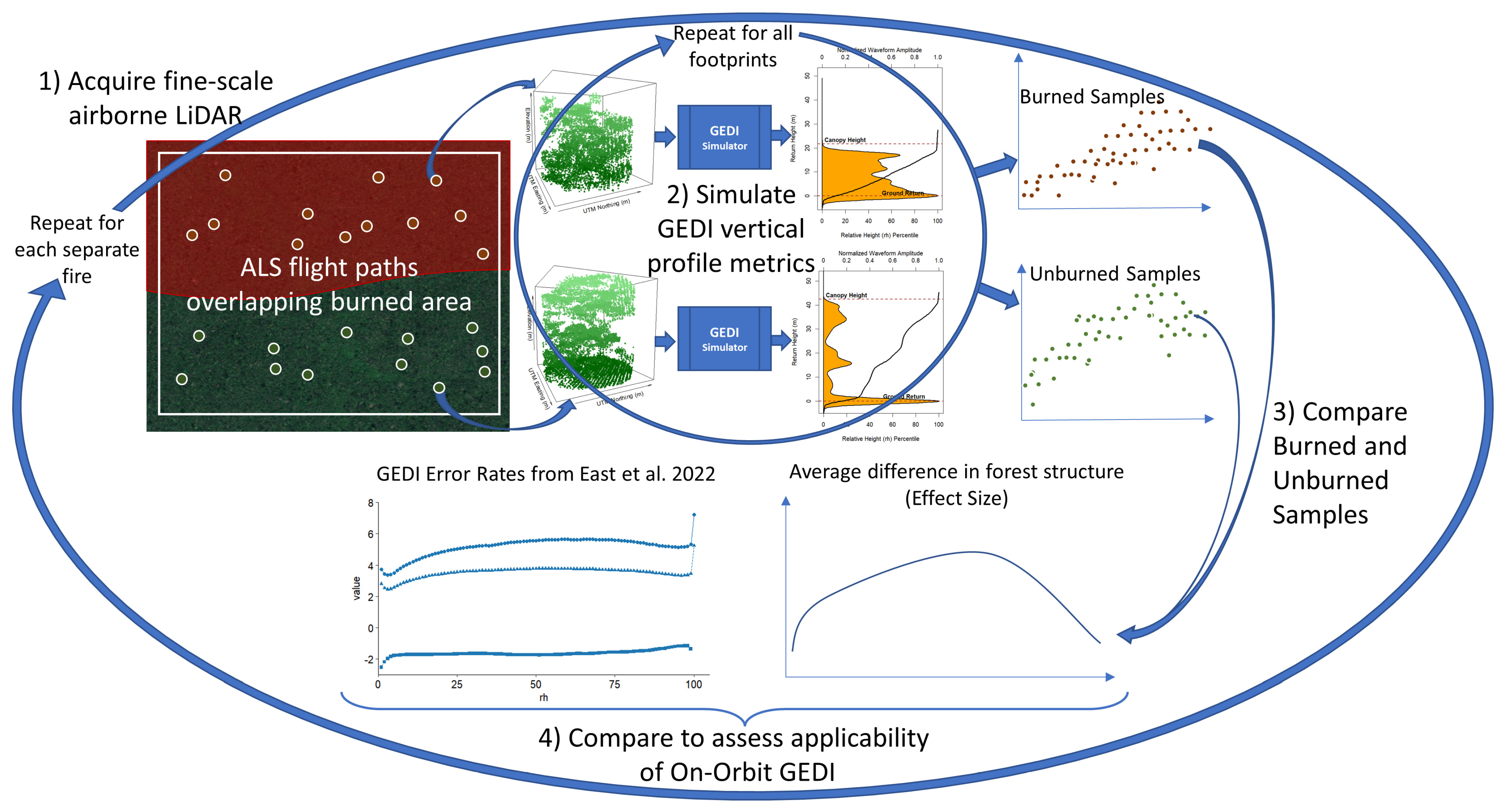
2.1. Concept and Workflow
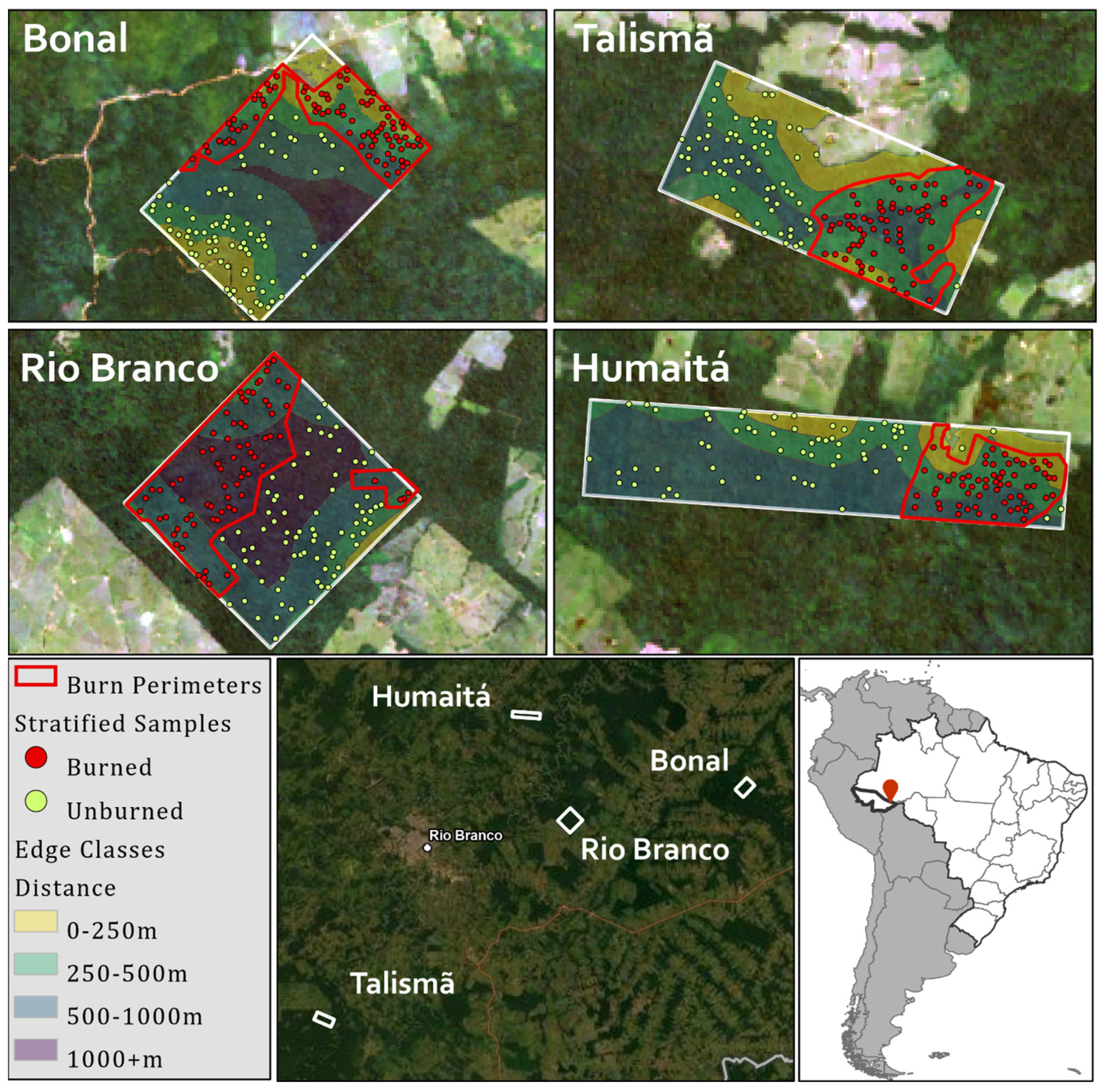
As a baseline, we employed well-validated airborne laser scanning (ALS) measurements from a previous study of the effects of four different previously documented understory fires on vegetation structure in Acre, Brazil [39]. That study quantified the overall change in average ALS height return and sampled forest composition by DBH classes [39]. We took a complementary and comparative view of these same fires through the lens of large-footprint LiDAR data. Fine-scale ALS data were used to simulate the corresponding large-footprint GEDI metrics of interest (Figure 1) [40]. Using simulated data allowed us to assess how the vertical canopy profile was influenced by fire, while eliminating the influence of measurement error that we knew existed in on-orbit GEDI data [35]. The changes in vertical distribution could then be compared to the previous regional measurements of GEDI error magnitudes to assess whether on-orbit GEDI data had the accuracy and sensitivity to detect the same changes seen in simulated data (Figure 1).

2.2. Study Area

The regions of interest fell within the state of Acre in southwestern Brazil (Figure 2). Study sites covered two distinct forest types: Bonal and Rio Branco (RIB) are open submontane rainforests with bamboo, while Humaitá and Talismã are dense submontane rainforests with emergent canopy [39]. These sites were chosen given the baseline investigation of the effect of fire on LiDAR response in Sato et al. (2016). Rio Branco and Humaitá were both disrupted by an understory fire in 2005, while Bonal and Talismã experienced an understory fire in 2010. All sites were then sampled by ALS LiDAR in 2013, giving a matrix of time post-burn and variation in forest type between sites (Table 1). These variations in the time since burn and forest type provided added nuance to the results of our analysis, and general trends among groups were considered in the interpretation of the results.

2.3. Data Inputs

2.3.1. Airborne Laser Scanning Data

ALS data were acquired in 2013 by the Sustainable Landscapes Brazil project [41] and are all open-source and freely available through the Oak Ridge National Laboratory (ORNL). Data were pre-processed as part of this project to filter noise, and were geolocated and corrected for the misalignment of overlapping flights [41]. The average spatial resolution was ~10 points per m2, and the total area covered was 2600 ha: Bonal (600 ha), Talismã (500 ha), Humaitá (500 ha), and Rio Branco (1000 ha) (Table A1).

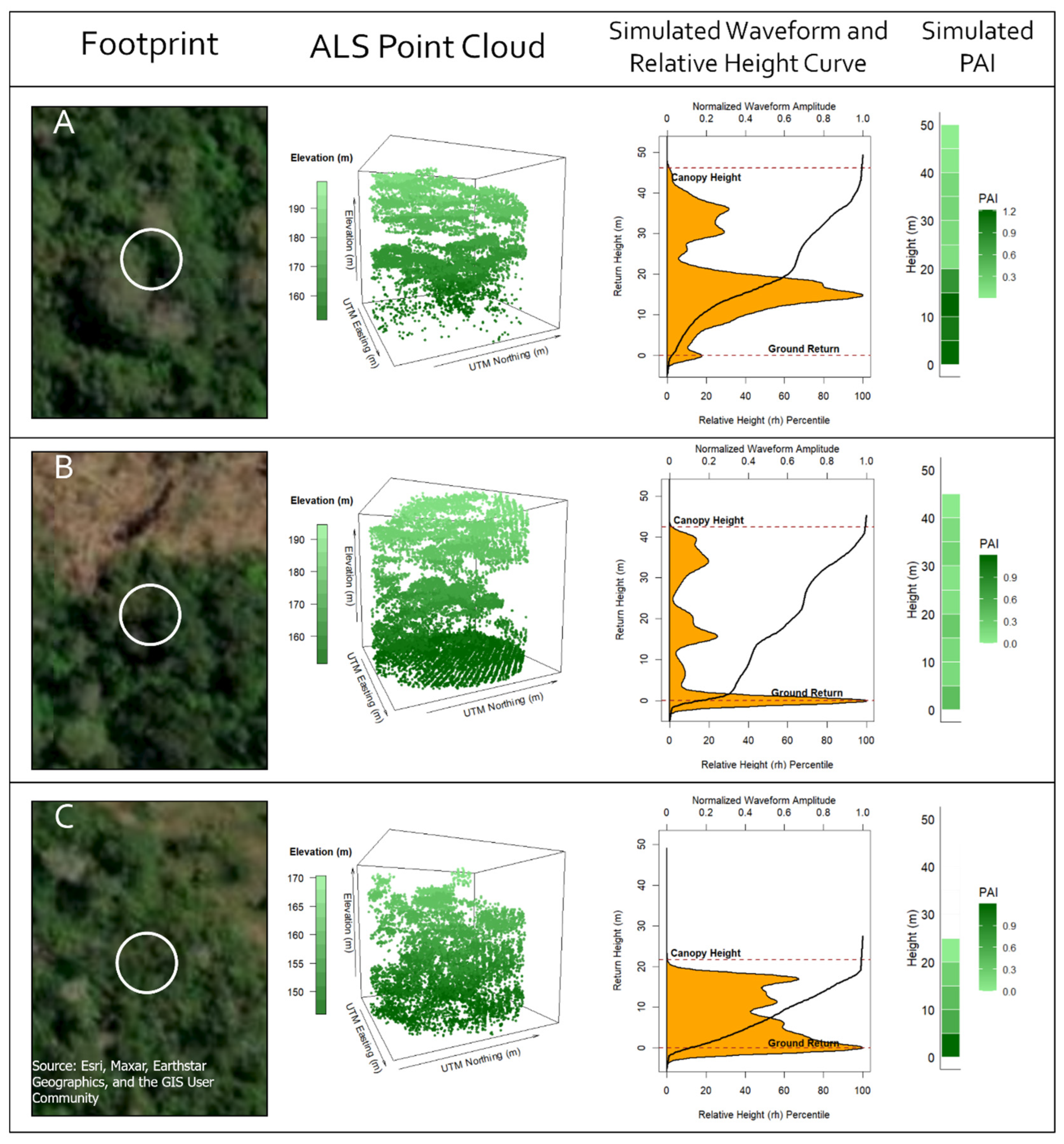
2.3.2. GEDI Simulation

Differences in vertical canopy structure between burned and unburned forest were quantified using two large-footprint LiDAR metrics: plant area index (PAI) and relative height (RH) curves. The randomly generated points were used for footprint centroids, and the corresponding ALS data were passed through the GEDI simulator algorithm to create 25-m-diameter footprints [40], corresponding to the GEDI L1B data product (Figure 3). Waveforms were further processed to derive the canopy height profile quantified by the GEDI relative height (RH) curve (GEDI L2A data product). This was performed at 1% step intervals based on the Gaussian ground finding algorithm [42]. Plant area index (PAI) was also simulated to represent the GEDI L2B data products [43] (Figure 3).
PAI has the benefit of easy interpretation, given its intuitive breakdown into height classes. PAI values were calculated for binned sections of the canopy by height in 5 m intervals (0–5 m, 5–10 m, …, 60–65 m), and the PAI value was a measure of the total estimated area covered by plant matter per ground area (m2m−2) within each bin.
Relative height metrics were calculated from a normalized cumulative distribution function of the waveform return, so that a height return represents the height above the ground at which a given percentage of the total waveform energy has occurred. For example, 50 percent of total waveform energy (denoted RH50) and the associated height return value represent the point in the relative height curve where 50% of the cumulative waveform energy has occurred (Figure 3) [35,44,45]. RH curves benefit from this normalized scale as it allows height return measurements to be compared across samples regardless of total canopy height (a limitation of PAI). This comparison provides insight into the relative change in distribution of the canopy as scaled from 0 to 100% of the canopy signal. RH measurements’ application is far-reaching; RH values are strongly associated with canopy structure and structural diversity, and are strong predictors of biomass [46,47,48]. Other studies have found RH metrics to be highly significant in identifying disturbance and classifying forest types [45,46]. Several RH metrics have established meanings based on the previous literature. RH98 measures total canopy height. RH50 represents the height above the ground at which half of the energy has been returned (the height of median energy) [46]. RH10 has proven to be sensitive to disturbance in past studies and has associated ecological interpretations (Table 2) [45]. Overall, positive changes in RH height returns are strongly associated with canopy growth, and decrease with loss. Additionally, the relative height comparison results can be more easily compared to regional GEDI error estimates (Section 2.5.3).
GEDI calibration can lead to negative height return values at the bottom of the RH range (e.g., below RH10). This is caused when the ground returns a significant portion of the laser energy [49]. We used the truncation method consistent with similar studies [50] to convert all negative values to NA, representing the ground.

2.4. Sampling Design

To control for the influence of edge effect, we employed a stratified random sample of points to use as centroids for simulated GEDI footprints. The stratified sampling considered burned and unburned as binary classifications (Section 2.4.1) and the distance from the forest edge (Section 2.4.2). Thirty points were randomly generated with a minimum distance of 60 m between points for each combination of edge zone and burn classification (Figure 2). The size and spatial configuration of burned areas sometimes did not allow 30 random points to fit. In these instances, the non-burned sample was randomly resampled to match the burn sample size. For some areas, this amounted to more points than others due to spatial configuration and the number of zones present based on distance from forest edge. However, the distribution of points between burned and unburned edge zones was constant (Table 3).

2.4.1. Fire Mapping

Burn scar perimeters were originally digitized by Sato et al. (2016) using a multistage approach. They first utilized the Moderate Resolution and Imaging Spectroradiometer (MODIS) eight-day averages to delineate course resolution changes throughout the fire season (June to November), and then added Landsat 5 and Landsat 7 imagery and linear spectral mixture models to improve spatial resolution. The Sato et al. (2016) burn scar delineations serve as the basis for classifying burned and unburned samples. We georeferenced the Sato et al. (2016) polygons to the ALS boundaries and utilized top-down digitization to recreate the burn perimeters. We also buffered the boundaries of the burn scars by 60 m (the along-track spacing of GEDI footprints) in either direction to reduce the chance of misclassification and limit spatial autocorrelation of adjacent points along the burn perimeter. Digitizing the Sato et al. (2016) site-specific burn perimeters as opposed to a more general fire-mapping data product (e.g., MODIS monthly burned area [51] or MAPBIOMAS burned area [52]) allows for direct comparison between studies. The MODIS and MAPBIOMAS products also yield different delineations of burned areas and appear to miss large portions of the fire scar polygon.

2.4.2. Forest Edge Classification

Sampling zones based on distance from the forest edge from the year of ALS acquisition (2013) controlled for the influences of edge effect. The forest/non-forest classifications were generated using a supervised minimum distance classification [53] of Landsat 8 Level 2 images (USGS) from 1 January to 31 December 2013, in Google Earth Engine [54]. Images were masked to remove cloud cover, and band medians were taken across all images from 2013 to produce a final image for classification. Areas of forest and non-forest were digitized top-down around the ALS sites, and training classes were tuned iteratively based on visual inspection. Overall, the classification was able to pick up the presence of small clearings and roads that were missed by other land cover data products. The small clearing and roads greatly impacted the distribution of distance from edge measurements. Euclidian distance from non-forested patches was calculated, and binned intervals were created with unequal breaks based on the nonlinear relationship between distance and edge effects [19,55]. These intervals represented the zones for stratified random sampling and resulted in 4 classes with the ranges 0 to 250 m, 250 to 500 m, 500 to 1000 m, and 1000+ m.

2.5. Statistical Analysis

2.5.1. Objective 1: Measure Changes in Canopy Structure

Wilcoxon’s unpaired two-sample signed-rank test was used to measure the estimated difference in medians and the 95% confidence intervals of PAI values for each height bin between burned and unburned samples at each site [56]. Wilcoxon’s test was chosen given the non-parametric distribution of the data. The tallest PAI height classes (above 45 m) had small sample sizes that were not viable for statistical tests (Table A2).
Negative binomial generalized additive models (GAMs) were used to assess whether the distribution of the relative height curve exhibits different trends between burned and unburned forest at each site individually [57]. The GAM for each site was given height return as the response variable and a smoothed spline for the interaction between the percent of waveform energy returned (RH%), with burn status as the predictor variable. To assess whether the interaction of burn status is a significant predictor of height returns throughout relative height percentiles, we analyzed the variance (ANOVA) in the model predictors [58].
To assess the relative response throughout canopy layers, we took the difference between the two predicted GAM fit lines (unburned–burned). A positive difference indicated that the unburned height return was higher than the burned height return at a given relative height percentile. This difference curve was then compared across the percent of total energy return gradient, with significance assessed as whether the 95% confidence interval intersected with zero. Because the height returns associated with lower canopy measurements were inherently smaller than those at the top of the canopy, we also converted these estimates to percent change. Percent change or relative change were calculated as the difference between GAM fit lines divided by the average height return at each percent of total energy return throughout the canopy.

2.5.2. Objective 2: Quantify Fire Severity

While GEDI does not resample points, it does have orbital crossovers that resample regions through time and, as such, there is the potential to look at the change in response to fire at the stand level. This application tests the potential for the stand-level assessment with a space-for-time substitution. The general approach of Hu et al. (2019) was to take an integrated area under the normalized profile curve of height percentiles from pre- to post-burn. The change in area under these two curves from pre- to post-burn measured the overall effect of the fire on the forest structure or the fire severity. To derive a fire severity metric from large-footprint LiDAR data, we proposed to modify the methods used in Hu et al. (2019) to apply them to the relative height values given by GEDI. GEDI’s L2A dataset’s relative height curves were broken down into steps of 1 percentile instead of a continuous curve.
While integration is computationally expensive, and in anticipation of potentially applying this method across a large GEDI dataset, we proposed to use a summation of all positive values of RH as an approximation of the same method.
RH int = i = 0 98 f ( RH i ) d RH i   RH sum = i = 0 98 RH i
This metric (RHsum) was calculated for each point in the dataset and analyzed for a difference in medians between the burned and unburned forest. This analysis was performed for each fire area using an unpaired two-sample Wilcoxon’s signed-rank test [56].

2.5.3. Objective 3: Assess Applicability of On-Orbit GEDI

The accuracy of on-orbit GEDI data is constrained by factors including geolocation errors, canopy height, density, and cloud cover. Several efforts have focused on establishing regional error rates and identifying drivers of these accuracy challenges [35,50,59,60]. By comparing the results from Objective 1 and 2 to Amazonian regional error magnitudes established in East et al. 2022, we could infer whether on-orbit GEDI has the sensitivity to capture the same results. The GEDI accuracy metrics of interest were based on comparing on-orbit GEDI data relative height curves to simulated GEDI relative height curves from across the Brazilian Amazon. These metrics included R-squared, root mean squared error (RMSE), mean absolute error (MAE), and absolute bias. R-squared is the most challenging to interpret directly in comparison to the data given that they do not share units but, instead, the R-squared values illuminated a general trend in the agreement between GEDI data and validation data. RMSE, MAE, and absolute bias were all measured in meters. RMSE and MAE measured the average expected error in the height return for a given percentile of energy return of on-orbit GEDI data. Absolute bias values indicated the skew of the on-orbit GEDI data compared to the validation data. We used absolute bias for scaling reasons because GEDI underestimates values leading to negative bias values. Error calculations came from a GEDI-ALS data comparison that utilized the same GEDI simulator program used in this application. Notably, this simulator also has inherent sources of error, so the actual error values are likely slightly lower than the data presented.
For Objective 1, the results of the difference between GAM fit lines for burned and unburned samples (e.g., the average change in relative height curve) were plotted and compared to the rates of GEDI R-squared, MAE, RMSE, and bias.
For Objective 2, the average differences in RHsum were also compared to the MAE, RMSE, and R-squared values for that metric as measured in East et al. (2022). In the accuracy assessment, there were multiple scenarios of data accuracy. Generally, the accuracies were higher in data with a simulated geolocation correction, and these are the numbers presented in this analysis.

3. Results

3.1. Changes in Canopy Structure

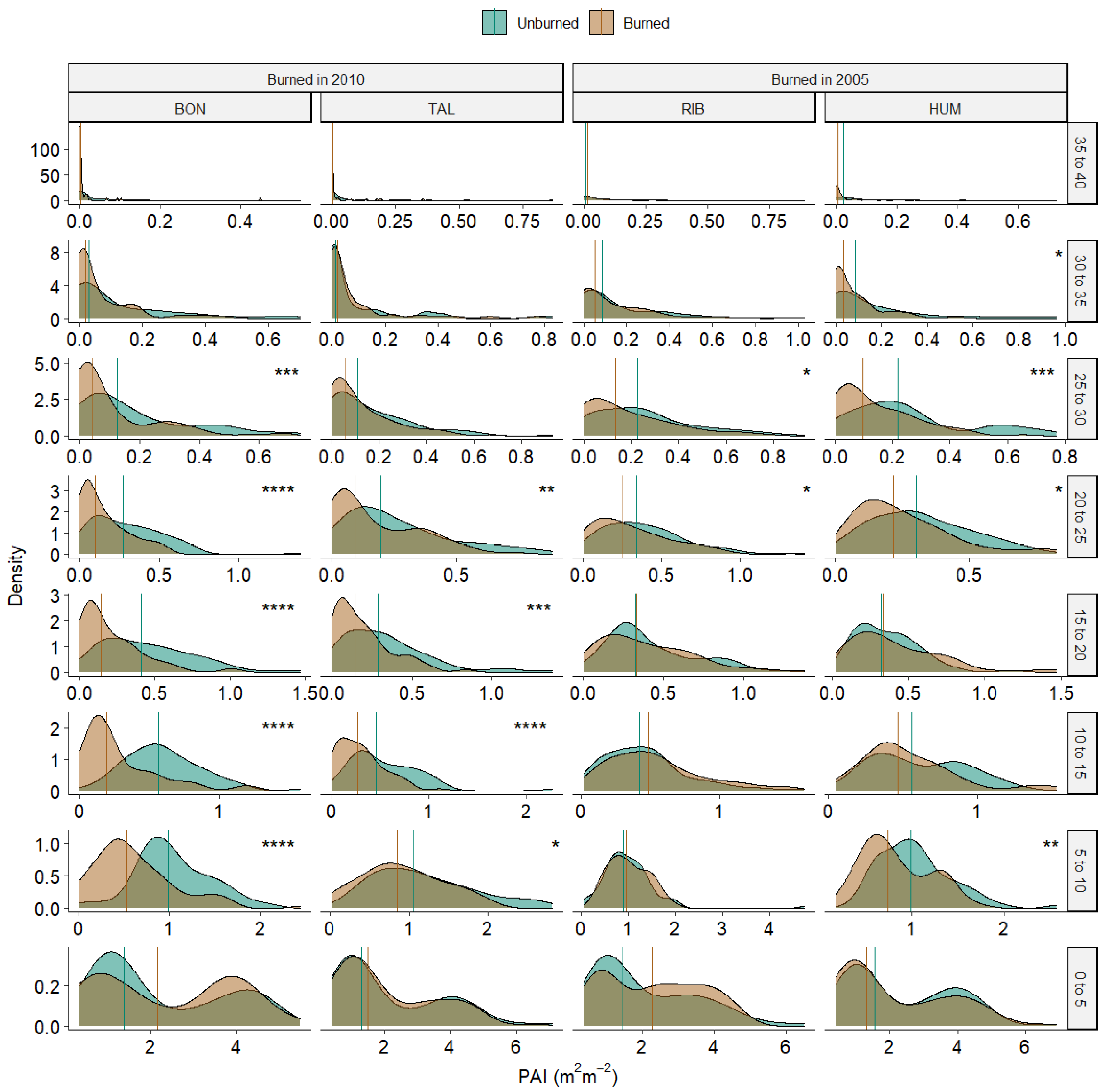
3.1.1. Plant Area Index Response

Across the analysis, the values of PAI and average height returns are decreased in burned sites. Sites that were 3 years post-burn (Bonal and Talismã) showed strong evidence of the greatest differences between burned and unburned PAI in the height bins from 5 to 10 up with significant differences in all height classes from 5 to 25 m (p-value < 0.001) (Figure 4). Bonal exhibited significant changes even higher into the 25-to-30-m-height class.
The 8-year-post-burn sites did not show the same significant differences in the lower canopy. Rio Branco had weak evidence of a difference in PAI values (p-values < 0.05) in the 20-to-25- and 25-to-30-height bins and no statistical differences anywhere else in the canopy (Figure 4). Humaitá shows evidence of a difference in PAI between burned and unburned sites in the 5-to-10-m-height bin, with unburned forest appearing higher than burned forest. There is weak evidence for the same trend in the 20-to-25-m- and the 25-to-30-m-height classes.
PAI difference shows a consistent trend in the 3-year-post-burn sites. The greatest estimated PAI differences (up to 0.45 m2m−2) start in almost the bottom of the canopy (5–10 m). The size of the PAI differences decreases into the upper canopy (Figure 5). This signal is less pronounced in the 8-year-post-burn sites, where the confidence intervals surrounding difference estimates are wider, but there are consistent differences in the canopy’s 20 to 30 m range (Figure 5).

3.1.2. Relative Height Curve Response

Relative height values are highly variable throughout the canopy, but the density distribution of these points shows that unburned samples are, on average, higher than burned samples (Figure 6). All of the generalized additive models identified the interaction of burn status and percent of waveform energy as being highly significant in predicting height for a given percentile (p-values < 0.0001). The deviance explained by the GAMs ranged from 67.2% (Rio Branco) to 74.5% (Bonal).
GAM fit lines reveal variability in canopy response throughout the canopy layers between sites (Figure 7). There are also two distinct shapes to these differences: peak and plateau. A peak is where there is a singly defined point of greatest difference between the fit lines, while a plateau shows a region of greatest difference that is consistent between two points.
The greatest difference between fit lines occurs in the Bonal site, where the height returns of unburned areas are as much as 6.6 m higher than burned samples. Bonal shows a plateau-shaped distribution with an area of maximum difference between two peaks, one at 48% of total energy retuned (RH48) and the other at 80% of total energy retuned (RH80), with an average value between them of 6.53 m (Figure 7). Talismã has a plateau of greatest difference falling between two peaks at 39% and 69% of total energy retuned (RH39 and RH69). The peak at 39% is lower but statistically indistinguishable (3.16 m difference, 95% CI 2.8–3.6) than that at 69% (2.95 m difference, 95% CI 2.3–3.6). The average between these points was 3.02 m. In both cases, this results in a decrease in the height of median energy. The top of the canopy appears to have less difference than the mid and lower canopy within the more recent burns. Talismã does not show a significant difference between burned and unburned classes above 95% of total energy returned.
The more recent burns (Bonal and Talismã) have a plateau response curve, while the sites that are eight years post-burn (Rio Branco and Humaitá) show a peak of greatest difference (Figure 7). Rio Branco shows a single peak at 73% total energy return (2.99 m difference, 95% CI 2.16–3.80). Humaitá shows the greatest difference at 78% total energy return (3.9 m difference, 95% CI 3.06–4.73). While the differences in the older burned sites have a skew toward the upper canopy, the top-of-canopy measurements of change still do not appear to be significant. In the case of Humaitá, the differences are not significant until RH97 and below, while for Rio Branco, differences are not significant below RH2 or above RH96.
Looking at the same responses as percent change in canopy height (Figure 8), there were similar differences between the fires based on time since burn. In both three-year-post-burn sites, there is an inverse relationship between percent change and percent of total energy return. Percent change shows a continuous decrease moving up through the canopy except for the lowest percentile values where there is a high density of ground returns, and the confidence intervals become wide. While Bonal shows much greater differences in height returns in the raw difference calculation, when scaled by average unburned height, the percent change was very similar between Bonal and Talismã (Figure 8).
Comparatively, in the eight-year-post-burn sites, we still see the greatest percent change in the lowest energy return percentiles for Humaitá, but both trends show a flattening between ~30% and 75% of total waveform energy. Rio Branco has a very low percent change throughout canopy layers, while Humaitá shows an increase in percent change in the lower canopy, similar to the 3-year sites. In all of the percent change trends, there was a degree of volatility in the lowest parts of the canopy due to the increasingly small height returns associated with these energy percentiles as they approached zero. As such, the highest percent change was in the very bottom of the canopy.

3.2. Fire Severity

Fire severity measurements (RHsum) show the largest differences in Bonal. Burned Bonal samples have a difference in median RHsum value of 501 lower than unburned samples (95% confidence interval, 336 to 639, p-value < 0.0001) (Figure 9). Talismã has an estimated difference in median of 229 m (95% confidence interval, 65 to 390, p-value = 0.006). Comparatively, the evidence for a true difference in medians was not as strong for the eight-year-post-burn areas. The difference in medians between burned and unburned areas was 171 m for Rio Branco (95% confidence interval, 1 to 343, p-value = 0.04) and 231 m for Humaitá (95% confidence interval, 77 to 338, p-value = 0.004).
While the difference in RHsum for Bonal is greater than all of the other sites, the values for Talismã, Rio Branco, and Humaitá are all very similar despite the consistent differences found between the 2010 fires (Talismã) and the 2005 fires (Rio Branco and Humaitá).

3.3. Applicability of On-Orbit GEDI

3.3.1. Burn Severity

In comparing the measured changes in RHsum, in the most severe fire (Bonal), the difference in medians of RHsum is 501 (95% confidence interval, 336 to 639). For this region, even under ideal accuracy scenarios, we expect an RMSE for RHsum of 423, which is within the 95% confidence interval of Bonal, and greater than the differences in the other three fires. As such, this easily derived fire severity metric is likely unsuitable for on-orbit GEDI data, even at the stand level.

3.3.2. Forest Structural Change

The measurement error in GEDI RH intervals was high, relative to differences in structure between burned and unburned stands for most stands and height intervals. The exception was Bonal, where the observed differences exceeded GEDI’s estimated RMSE and MAE. The lower confidence interval around the Bonal response curve crosses the GEDI RMSE curve between 30 and 82% of total waveform energy return (RH33 and RH82) (Figure 10). Thus, we can infer that on-orbit GEDI data may detect the greatest structural differences in the Bonal fire. However, the effects of fires at the other three sites are more of a challenge. GEDI absolute bias values are largely below the differences detected in the three sites. The nonlinearity of bias in the lower canopy has the potential to distort the shape of the overall response curve.

4. Discussion

4.1. Fire Effects

Burned samples were reduced in PAI and RH compared to unburned samples, especially in mid-canopy height ranges. Only the Bonal fire appears to have had any change in the top of canopy height as measured by RH98, while all fires showed the largest decrease in the mid to upper canopy, and a consistent decrease in height of median energy RH50. The decrease in median height with no change in total height may indicate a decrease in canopy evenness as measured by an increase in the vertical distribution ratio (VDR) [61]. High VDR has also been negatively associated with habitat for forest-endemic tropical bird species [62]. RH10 is also reduced by fire, indicating a decrease in canopy density and canopy cover. These effects were greatest in the most recently burned stands, but the progression upwards through canopy layers in both PAI and RH is consistent with delayed mortality and fire time-lag effects [17,63]. This indicates that, while there is recovery, the effects of fire, even that of low-severity fire, persist well into the future and may have long-lasting consequences.
These results are particularly interesting when compared to the changes in the distribution of DBH classes from field measurements due to fire. Previous studies identify DBH and bark thickness as the primary determinants of fire-induced mortality, with height explaining less but still a significant amount of variation in this relationship [63,64]. We capture some of this variability in our results. Sato et al. (2016) identified a decrease in the larger diameter trees (25–40 cm DBH). However, there was no detected effect on the largest diameter trees (>40 cm DBH) [39]. Simulated GEDI footprints do appear to capture the loss of the larger trees as accounted for in the mid-canopy differences, but the top of canopy measurements do not exhibit the same degree of change, likely because those largest emergent trees remain intact. Additionally, all sites showed an increase in small-diameter trees in the lower-size classes (10–25 cm DBH) [39]. Despite this, we still see a very small decrease with fires in the bottom canopy measurements and a decrease in PAI in the 5-to-10-m-height class. This could indicate one or two things: either that large-footprint LiDAR is not capturing this regeneration and change in forest composition in its three-dimensional profile, or that this regeneration still amounts to less overall biomass in lower canopy layers than the unburned forest. Notably, in the plant area index measurements for 0 to 5 m, the median values of burned forest were higher than that of unburned forest with striking bimodal distributions; however, this difference in medians was not significant according to Wilcoxon’s ranked sign test. The 0 to 5 m bin also presents potential challenges for accurate PAI measurements due to the influence of the ground signal.
These four fires also have variability in forest composition, with two characterized as open forests with bamboo, and the others characterized as dense forests with emergent structures (Table 1). Other studies of fire effects in the Amazon region document complex changes in species community structure in response to fire [22,38,65,66]. In an assessment of fires in this region of Acre, there is specific documentation of an increase in pioneer species Cecropia sp., Urera sp., Phenakosperumu guyannense, Bixa urucurana, and bamboo in response to fire [66]. In addition to overall species composition changes, the presence of bamboo is known to change the overall structure and response of forests to fire [67,68,69]. The 0-to-5-m-PAI-height classes in the Bonal and Rio Branco sites (characterized by dense bamboo patches) exhibit a bimodal distribution and a higher (but non-significant) median PAI in burned sites. The influence of bamboo on forest structure and regeneration may explain this phenomenon, but this relationship would need to be studied further, especially given the challenges associated with detangling PAI from ground return signals in large-footprint LiDAR data.

4.2. Applications of On-Orbit GEDI

Given that GEDI accuracy is highest at the top of the canopy and deteriorates as relative height percentile decreases, it is initially promising that most of the relative height differences occur in the mid-canopy, where R-squared values are reasonable. However, when comparing GEDI RMSE and MAE with detected differences in stand-level relative height trends, three out of four sites have differences that never exceed GEDI RMSE or MAE. In comparison, all of the differences detected exceed the rates of GEDI absolute bias. The nonlinearity of the bias presents additional problems, given the importance of the response curve shapes. The error metrics of RMSE, MAE, bias, and R-squared all come from a comparison of GEDI data to simulated GEDI data, which introduces its own source of error. Thus, the true error rates are likely slightly lower than those presented here. However, given the degree to which the error rates exceed the fire effect sizes, we can infer that on-orbit GEDI data may be able to measure changes in more severe fires, but the nuances of low-severity understory fires may go largely undetected.
These findings do not rule out all applications of on-orbit GEDI data in fire ecology or other disturbance studies. For example, efforts that aim to classify forests into categories such as disturbed or undisturbed have already proven promising [29], and data fusion with spectral products often increases predictive power. Moving forward, some of the challenges to consider include through-canopy accuracy, regional differences in GEDI data accuracies [35,59], and geolocation errors (particularly in fragmented habitats) [36]. The ability of remote sensing to accurately detect and map fire occurrence is still limited. These limitations lead to errors of omission and commission in existing burned area mapping [70], and such errors could compound the challenges of GEDI sensitivity. For example, in this study we used highly localized fire polygons that were created interactively and individually inspected [39]. The global or regional products available omitted large sections of the burn scar compared to the Sato et al. polygons. Such differences in burned area mapping could lead to the misclassification of many samples, and potentially very different results.
Further work is also needed to assess the viability of using PAI or biomass estimates from GEDI for understory fires. PAI showed similar results to the relative height differences, and likely has different accuracy rates from the relative height data given its algorithmic derivation [71]. A recent evaluation of GEDI PAI and plant area volume density over southeastern Australia indicates that the accuracy of these metrics also varies through canopy layers [72]. They specifically identify accuracy challenges below 30 m in height for those forests, consequently, where we see the largest effects of fire in our results. It was outside the scope of this work to assess the accuracy of these metrics; however, there is an indication that such an evaluation could prove to be informative.

4.3. Conclusions

This is the first study we are aware of that both used simulated GEDI data to investigate ecological effects and took the additional step of comparing these findings with a regional assessment of on-orbit GEDI accuracy. In this application, we focused on understory fire, one of the most challenging fire types to measure using remote sensing. Overall, we found mixed results for applications of on-orbit GEDI data to tropical fire. While simulated large-footprint GEDI data provide a novel look into the effects of understory fire on canopy structure, these data did not capture the intricacies of regeneration. We were able to detect the greatest differences in canopy metrics in the mid to lower canopy, with time-lag dynamics shifting those differences upward in the canopy with time. Our analysis was also limited to areas that burned 3 to 8 years previously; we could not assess how the canopy profile would have changed directly following fire due to data constraints. However, given the relatively small effect size in terms of meter difference through canopy measurements, it is unlikely that GEDI’s relative height product has the data accuracy to detect the same changes. There is still the open question of the ability of GEDI’s plant area index data product and above-ground biomass product to accurately detect temporal changes with regard to fire.

Author Contributions

Conceptualization, A.E.; methodology, A.E., D.A. and P.J.; formal analysis, A.E.; data curation, A.E.; writing—original draft preparation, A.E.; writing—review and editing, A.H., D.W.R., P.J. and D.A.; visualization, A.E.; supervision, A.H., D.W.R., P.J. and D.A.; funding acquisition, A.E. All authors have read and agreed to the published version of the manuscript.

Funding

This research was partially funded by Montana Space Grant Contortion Graduate Fellowship: 80NSSC20M0042. The APC was funded by The Montana State University Open Access Author Fund.

Data Availability Statement

Publicly available datasets were analyzed in this study. These data can be found here: https://daac.ornl.gov/cgi-bin/dsviewer.pl?ds_id=1644 (accessed on 7 December 2021).

Acknowledgments

Computational efforts were performed on the Hyalite High Performance Computing System, and operated and supported by the University Information Technology Research Cyberinfrastructure at Montana State University.

Conflicts of Interest

The authors declare no conflict of interest.

Appendix A

Table A1. Information in ALS data including acquisition data, average point density, area coverage, and flight codes. Data come from the Sustainable Landscapes GeoNetwork Catalog.
Site NameFlight CodesNumber of ALS TilesArea CoveredAverage Return Density (points/m2)Date (Day–Month–Year)
BonalBON_A01_2013_LiDAR14600 ha33.3916 September 2013
HumaitáHUM_A01_2013_LiDAR12500 ha66.6115 September 2013
Rio BrancoRIB_A01_2014_LiDAR181000 ha71.7412 April 2015
TalismãTAL_A01_2013_LiDAR12500 ha40.729 May 2014
Table A2. Distribution of samples containing PAI observations by height bin.
0–55–1010–1515–2020–2525–3030–3535–4040–4545–5050–5555–60
Burned288288288287287282253190851731
Unburned2882882882872862852712131102960

References

  1. Laurance, W.F. A Crisis in the Making: Responses of Amazonian Forests to Land Use and Climate Change. Trends Ecol. Evol. 1998, 13, 411–415. [Google Scholar] [CrossRef] [PubMed]
  2. Cochrane, M.A.; Schulze, M.D. Fire as a Recurrent Event in Tropical Forests of the Eastern Amazon: Effects on Forest Structure, Biomass, and Species Composition. Biotropica 1999, 31, 2–16. [Google Scholar] [CrossRef]
  3. Longo, M.; Keller, M.; dos-Santos, M.N.; Leitold, V.; Pinagé, E.R.; Baccini, A.; Saatchi, S.; Nogueira, E.M.; Batistella, M.; Morton, D.C. Aboveground Biomass Variability across Intact and Degraded Forests in the Brazilian Amazon. Glob. Biogeochem. Cycles 2016, 30, 1639–1660. [Google Scholar] [CrossRef] [Green Version]
  4. Curtis, P.G.; Slay, C.M.; Harris, N.L.; Tyukavina, A.; Hansen, M.C. Classifying Drivers of Global Forest Loss. Science 2018, 361, 1108–1111. [Google Scholar] [CrossRef] [PubMed]
  5. Matricardi, E.A.T.; Skole, D.L.; Costa, O.B.; Pedlowski, M.A.; Samek, J.H.; Miguel, E.P. Long-Term Forest Degradation Surpasses Deforestation in the Brazilian Amazon. Science 2020, 369, 1378–1382. [Google Scholar] [CrossRef]
  6. Morgan, W.T.; Darbyshire, E.; Spracklen, D.; Artaxo, P.; Coe, H. Non-Deforestation Drivers of Fires Are Increasingly Important Sources of Aerosol and Carbon Dioxide Emissions across Amazonia. Sci. Rep. 2019, 9, 1–15. [Google Scholar] [CrossRef] [Green Version]
  7. Cochrane, M.A.; Alencar, A.; Schulze, M.D.; Souza, C.M.; Nepstad, D.C.; Lefebvre, P.; Davidson, E.A. Positive Feedbacks in the Fire Dynamic of Closed Canopy Tropical Forests. Science 1999, 284, 1832–1835. [Google Scholar] [CrossRef]
  8. Hoffmann, W.A.; Jaconis, S.Y.; Mckinley, K.L.; Geiger, E.L.; Gotsch, S.G.; Franco, A.C. Fuels or Microclimate? Understanding the Drivers of Fire Feedbacks at Savanna-Forest Boundaries. Austral Ecol. 2012, 37, 634–643. [Google Scholar] [CrossRef]
  9. Alencar, A.; Nepstad, D.; del Carmen Vera Diaz, M. Forest Understory Fire in the Brazilian Amazon in ENSO and Non-ENSO Years: Area Burned and Committed Carbon Emissions. Earth Interact. 2006, 10, 1–17. [Google Scholar] [CrossRef]
  10. Jimenez, J.C.; Libonati, R.; Peres, L.F. Droughts Over Amazonia in 2005, 2010, and 2015: A Cloud Cover Perspective. Front. Earth Sci. 2018, 6, 1–7. [Google Scholar] [CrossRef] [Green Version]
  11. Cox, P.M.; Betts, R.A.; Collins, M.; Harris, P.P.; Huntingford, C.; Jones, C.D. Amazonian Forest Dieback under Climate-Carbon Cycle Projections for the 21st Century. Appl. Clim. 2004, 78, 137–156. [Google Scholar] [CrossRef]
  12. Nobre, C.; Obregón, G.; Marengo, J.; Fu, R.; Poveda, G. Characteristics of Amazonian Climate: Main Features. In Amazonia and Global Change; Keller, M., Bustamante, M., Gash, J., Silva Dias, P., Eds.; John Wiley & Sons, Inc.: Hoboken, NJ, USA, 2009. [Google Scholar]
  13. Wright, S.J. Plant Diversity in Tropical Forests: A Review of Mechanisms of Species Coexistence. Oecologia 2002, 130, 1–14. [Google Scholar] [CrossRef]
  14. Global Fire Emissions Database Amazon Dashboard. Available online: https://globalfiredata.org/pages/amazon-dashboard/ (accessed on 1 April 2021).
  15. Rappaport, D.I.; Morton, D.C.; Longo, M.; Keller, M.; Dubayah, R.; Dos-Santos, M.N. Quantifying Long-Term Changes in Carbon Stocks and Forest Structure from Amazon Forest Degradation. Environ. Res. Lett. 2018, 13, 065013. [Google Scholar] [CrossRef]
  16. Barlow, J.; Peres, C.A. Ecological Responses to El Niño-Induced Surface Fires in Central Brazilian Amazonia: Management Implications for Flammable Tropical Forests. Philos. Trans. R. Soc. B Biol. Sci. 2004, 359, 367–380. [Google Scholar] [CrossRef]
  17. Silva, C.V.J.; Aragão, L.E.O.C.; Barlow, J.; Espirito-Santo, F.; Young, P.J.; Anderson, L.O.; Berenguer, E.; Brasil, I.; Brown, I.F.; Castro, B.; et al. Drought-Induced Amazonian Wildfires Instigate a Decadal-Scale Disruption of Forest Carbon Dynamics. Philos. Trans. R. Soc. B Biol. Sci. 2018, 8, 373. [Google Scholar] [CrossRef] [Green Version]
  18. Silva, C.H.L.; Aragão, L.E.O.C.; Anderson, L.O.; Fonseca, M.G.; Shimabukuro, Y.E.; Vancutsem, C.; Achard, F.; Beuchle, R.; Numata, I.; Silva, C.A.; et al. Persistent Collapse of Biomass in Amazonian Forest Edges Following Deforestation Leads to Unaccounted Carbon Losses. Sci. Adv. 2020, 6, aaz8360. [Google Scholar] [CrossRef]
  19. Laurance, W.F.; Nascimento, H.E.M.; Laurance, S.G.; Andrade, A.C.; Fearnside, P.M.; Ribeiro, J.E.L.; Capretz, R.L. Rain Forest Fragmentation and the Proliferation of Successional Trees. Ecology 2006, 87, 469–482. [Google Scholar] [CrossRef]
  20. Malcolm, J.R. Edge Effects in Central Amazonian Forest Fragments. Ecology 1994, 75, 2438–2445. [Google Scholar]
  21. Nepstad, D.C.; Stickler, C.M.; Soares-Filho, B.; Merry, F. Interactions among Amazon Land Use, Forests and Climate: Prospects for a near-Term Forest Tipping Point. Philos. Trans. R. Soc. B Biol. Sci. 2008, 363, 1737–1746. [Google Scholar] [CrossRef] [Green Version]
  22. Armenteras, D.; Meza, M.C.; González, T.M.; Oliveras, I.; Balch, J.K.; Retana, J. Fire Threatens the Diversity and Structure of Tropical Gallery Forests. Ecosphere 2021, 12, 3347. [Google Scholar] [CrossRef]
  23. Miller, J.D.; Thode, A.E. Quantifying Burn Severity in a Heterogeneous Landscape with a Relative Version of the Delta Normalized Burn Ratio (DNBR). Remote Sens. Environ. 2007, 109, 66–80. [Google Scholar] [CrossRef]
  24. Roy, D.P.; Boschetti, L.; Trigg, S.N. Remote Sensing of Fire Severity: Assessing the Performance of the Normalized Burn Ratio. IEEE Geosci. Remote Sens. Lett. 2006, 3, 112–116. [Google Scholar] [CrossRef] [Green Version]
  25. Hu, T.; Ma, Q.; Su, Y.; Battles, J.J.; Collins, B.M.; Stephens, S.L.; Kelly, M.; Guo, Q. A Simple and Integrated Approach for Fire Severity Assessment Using Bi-Temporal Airborne LiDAR Data. Int. J. Appl. Earth Obs. Geoinf. 2019, 78, 25–38. [Google Scholar] [CrossRef]
  26. García, M.; North, P.; Viana-Soto, A.; Stavros, N.E.; Rosette, J.; Martín, M.P.; Franquesa, M.; González-Cascón, R.; Riaño, D.; Becerra, J.; et al. Evaluating the Potential of LiDAR Data for Fire Damage Assessment: A Radiative Transfer Model Approach. Remote Sens. Environ. 2020, 247, 111893. [Google Scholar] [CrossRef]
  27. Fernandez-Manso, A.; Quintano, C.; Roberts, D.A. Burn Severity Analysis in Mediterranean Forests Using Maximum Entropy Model Trained with EO-1 Hyperion and LiDAR Data. ISPRS J. Photogramm. Remote Sens. 2019, 155, 102–118. [Google Scholar] [CrossRef]
  28. Chuvieco, E.; Aguado, I.; Salas, J.; García, M.; Yebra, M.; Oliva, P. Satellite Remote Sensing Contributions to Wildland Fire Science and Management. Curr. For. Rep. 2020, 6, 81–96. [Google Scholar] [CrossRef]
  29. Liu, M.; Popescu, S.; Malambo, L. Feasibility of Burned Area Mapping Based on ICESAT-2 Photon Counting Data. Remote Sens. 2020, 12, 24. [Google Scholar] [CrossRef] [Green Version]
  30. Skowronski, N.S.; Gallagher, M.R.; Warner, T.A. Decomposing the Interactions between Fire Severity and Canopy Fuel Structure Using Multi-Temporal, Active, and Passive Remote Sensing Approaches. Fire 2020, 3, 7. [Google Scholar] [CrossRef] [Green Version]
  31. Pontes-Lopes, A.; Dalagnol, R.; Dutra, A.C.; de Jesus Silva, C.V.; de Alencastro Graça, P.M.L.; de Oliveira e Cruz de Aragão, L.E. Quantifying Post-Fire Changes in the Aboveground Biomass of an Amazonian Forest Based on Field and Remote Sensing Data. Remote Sens. 2022, 14, 1545. [Google Scholar] [CrossRef]
  32. Dubayah, R.; Blair, J.B.; Goetz, S.; Fatoyinbo, L.; Hansen, M.; Healey, S.; Hofton, M.; Hurtt, G.; Kellner, J.; Luthcke, S.; et al. The Global Ecosystem Dynamics Investigation: High-Resolution Laser Ranging of the Earth’s Forests and Topography. Sci. Remote Sens. 2020, 1, 100002. [Google Scholar] [CrossRef]
  33. Beck, J.; Armston, J.; Hofton, M.; Luthcke, S. GLOBAL Ecosystem Dynamics Investigation (GEDI) Level 02 User Guide For SDPS PGEVersion 1 (P001) of GEDI L2A Data and SDPS PGE Version 1 (P001) of GEDI L2B Data; 2020; Volume 1.0. Available online: https://lpdaac.usgs.gov/documents/589/GEDIL02_User_Guide_V1.pdf (accessed on 1 March 2022).
  34. Leite, R.V.; Silva, C.A.; Broadbent, E.N.; do Amaral, C.H.; Liesenberg, V.; de Almeida, D.R.A.; Mohan, M.; Godinho, S.; Cardil, A.; Hamamura, C.; et al. Large Scale Multi-Layer Fuel Load Characterization in Tropical Savanna Using GEDI Spaceborne Lidar Data. Remote Sens. Environ. 2022, 268, 112764. [Google Scholar] [CrossRef]
  35. East, A.; Hansen, A.J.; Jantz, P.A.; Roberts, D.; Armenteras-Pascual, D. Validation and Error Minimization of GEDI Data in the Amazon. Remote Sens. Environ. 2022; in review. [Google Scholar]
  36. Roy, D.P.; Kashongwe, H.B.; Armston, J. The Impact of Geolocation Uncertainty on GEDI Tropical Forest Canopy Height Estimation and Change Monitoring. Sci. Remote Sens. 2021, 4, 100024. [Google Scholar] [CrossRef]
  37. Balch, J.K.; Nepstad, D.C.; Curran, L.M.; Brando, P.M.; Portela, O.; Guilherme, P.; Reuning-Scherer, J.D.; de Carvalho, O. Size, Species, and Fire Behavior Predict Tree and Liana Mortality from Experimental Burns in the Brazilian Amazon. Ecol. Manag. 2011, 261, 68–77. [Google Scholar] [CrossRef]
  38. Santos, R.; Galvão, L.S.; Journal, S.; November, N.; Ramos, S.; Martins, V.; Abrahim, H.; Xaud, M.; Roberto, J. Effects of Fire on Above-Ground Forest Biomass in the Northern Brazilian Amazon. J. Trop. Ecol. 2012, 28, 591–601. [Google Scholar] [CrossRef] [Green Version]
  39. Sato, L.Y.; Gomes, V.C.F.; Shimabukuro, Y.E.; Keller, M.; Arai, E.; dos-Santos, M.N.; Brown, I.F.; de Aragão, L.E.O.e.C. Post-Fire Changes in Forest Biomass Retrieved by Airborne LiDAR in Amazonia. Remote Sens. 2016, 8, 839. [Google Scholar] [CrossRef] [Green Version]
  40. Hancock, S.; Armston, J.; Hofton, M.; Sun, X.; Tang, H.; Duncanson, L.I.; Kellner, J.R.; Dubayah, R. The GEDI Simulator: A Large-Footprint Waveform Lidar Simulator for Calibration and Validation of Spaceborne Missions. Earth Space Sci. 2019, 6, 294–310. [Google Scholar] [CrossRef]
  41. Dos-Santos, M.N.; Keller, M.M.; Morton, D.C. LiDAR Surveys over Selected Forest Research Sites, Brazilian Amazon, 2008–2018. 2019. Available online: https://daac.ornl.gov/CMS/guides/LiDAR_Forest_Inventory_Brazil.html (accessed on 8 November 2022).
  42. Hofton, M.A.; Minster, J.B.; Blair, J.B. Decomposition of Laser Altimeter Waveforms. IEEE Trans. Geosci. Remote Sens. 2000, 38, 1989–1996. [Google Scholar] [CrossRef]
  43. Tang, H.; Dubayah, R.; Swatantran, A.; Hofton, M.; Sheldon, S.; Clark, D.B.; Blair, B. Retrieval of Vertical LAI Profiles over Tropical Rain Forests Using Waveform Lidar at La Selva, Costa Rica. Remote Sens Environ. 2012, 124, 242–250. [Google Scholar] [CrossRef]
  44. Blair, J.B.; Hofton, M.A. Modeling Laser Altimeter Return Waveforms over Complex Vegetation Using High-Resolution Elevation Data. Geophys. Res. Lett. 1999, 26, 2509–2512. [Google Scholar] [CrossRef]
  45. Boucher, P.B.; Hancock, S.; Orwig, D.A.; Duncanson, L.; Armston, J.; Tang, H.; Krause, K.; Cook, B.; Paynter, I.; Li, Z.; et al. Detecting Change in Forest Structure with Simulated GEDI Lidarwaveforms: A Case Study of the Hemlock Woolly Adelgid (HWA.; Adelges Tsugae) Infestation. Remote Sens. 2020, 12, 1304. [Google Scholar] [CrossRef] [Green Version]
  46. Dubayah, R.O.; Sheldon, S.L.; Clark, D.B.; Hofton, M.A.; Blair, J.B.; Hurtt, G.C.; Chazdon, R.L. Estimation of Tropical Forest Height and Biomass Dynamics Using Lidar Remote Sensing at La Selva, Costa Rica. J. Geophys. Res. Biogeosci. 2010, 115, 1–17. [Google Scholar] [CrossRef]
  47. Duncanson, L.; Kellner, J.R.; Armston, J.; Dubayah, R.; Minor, D.M.; Hancock, S.; Healey, S.P.; Patterson, P.L.; Saarela, S.; Marselis, S.; et al. Aboveground Biomass Density Models for NASA’s Global Ecosystem Dynamics Investigation (GEDI) Lidar Mission. Remote Sens. Environ. 2022, 270, 112845. [Google Scholar] [CrossRef]
  48. Schneider, F.D.; Ferraz, A.; Hancock, S.; Duncanson, L.I.; Dubayah, R.O.; Pavlick, R.P.; Schimel, D.S. Towards Mapping the Diversity of Canopy Structure from Space with GEDI. Environ. Res. Lett. 2020, 15, 115006. [Google Scholar] [CrossRef]
  49. Beck, J.; Wirt, B.; Armston, J.; Hofton, M.; Luthcke, S.; Tang, H. GLOBAL Ecosystem Dynamics Investigation (GEDI) Level 2 User Guide For SDPS PGEVersion 3 (P003) of GEDI L2A Data and SDPS PGEVersion 3 (P003) of GEDI L2B Data Deputy Principal Investigator and Instrument Scientist User Guide Written by Jared Beck 3 in Coll. 2021; Volume 3, pp. 1–25. Available online: https://lpdaac.usgs.gov/documents/986/GEDI02_UserGuide_V2.pdf (accessed on 2 June 2022).
  50. Liu, A.; Cheng, X.; Chen, Z. Performance Evaluation of GEDI and ICESat-2 Laser Altimeter Data for Terrain and Canopy Height Retrievals. Remote Sens Environ. 2021, 264, 112571. [Google Scholar] [CrossRef]
  51. Giglio, L.; Justice, C.; Boschetti, L.; Roy, D. MCD64A1 MODIS/Terra+Aqua Burned Area Monthly L3 Global 500m SIN Grid V006 [Data Set]. NASA EOSDIS Land Process. DAAC 2015. Available online: https://lpdaac.usgs.gov/products/mcd64a1v006/ (accessed on 18 November 2020).
  52. Alencar, A.A.; Conciani, D.E.; Costa, D.P.; Rosa, E.R.; Martin, E.V.; Hasenack, H.; Martenexen, L.F.M.; Shimbo, J.; Rosa, M.; Crusco, N.; et al. MapBiomas Fire. Algorithm Theoretical Basis Document (ATBD). Collection 1.0. Development 2021. pp. 1–19. Available online: https://mapbiomas-br-site.s3.amazonaws.com/ATBD_MapBiomas_Fogo_Cole%C3%A7%C3%A3o_1.pdf (accessed on 7 December 2021).
  53. Wacker, A.G.; Landgrebe, D.A. Minimum Distance Classification in Remote Sensing. LARS Technical Reports. 1972, p. 25. Available online: https://docs.lib.purdue.edu/cgi/viewcontent.cgi?article=1024&context=larstech (accessed on 20 April 2022).
  54. Gorelick, N.; Hancher, M.; Dixon, M.; Ilyushchenko, S.; Thau, D.; Moore, R. Google Earth Engine: Planetary-Scale Geospatial Analysis for Everyone. Remote Sens. Environ. 2017, 202, 18–27. [Google Scholar] [CrossRef]
  55. Broadbent, E.N.; Asner, G.P.; Keller, M.; Knapp, D.E.; Oliveira, P.J.C.; Silva, J.N. Forest Fragmentation and Edge Effects from Deforestation and Selective Logging in the Brazilian Amazon. Biol. Conserv. 2008, 141, 1745–1757. [Google Scholar] [CrossRef]
  56. Wilcoxon, F. Individual Comparisons by Ranking Methods. Biom. Bull. 1945, 1, 80–83. [Google Scholar] [CrossRef]
  57. Hastie, T.; Tibshirani, R. Generalized Additive Models. Stat. Sci. 1990, 1, 297–318. [Google Scholar]
  58. Tukey, J.W. Comparing Individual Means in the Analysis of Variance. Biometrics 1949, 5, 99–114. [Google Scholar] [CrossRef]
  59. Wang, C.; Elmore, A.J.; Numata, I.; Cochrane, M.A.; Shaogang, L.; Huang, J.; Zhao, Y.; Li, Y. Factors Affecting Relative Height and Ground Elevation Estimations of GEDI among Forest Types across the Conterminous USA. GIsci. Remote Sens. 2022, 59, 975–999. [Google Scholar] [CrossRef]
  60. Fayad, I.; Baghdadi, N.; Riedi, J. Quality Assessment of Acquired Gedi Waveforms: Case Study over France, Tunisia and French Guiana. Remote Sens. 2021, 13, 3144. [Google Scholar] [CrossRef]
  61. Goetz, S.J.; Steinberg, D.; Betts, M.G.; Holmes, R.T.; Doran, P.J.; Dubayah, R.; Hofton, M. Lidar Remote Sensing Variables Predict Breeding Habitat of a Neotropical Migrant Bird. Ecology 2010, 91, 1569–1576. [Google Scholar] [CrossRef]
  62. Singh, M.; Tokola, T.; Hou, Z.; Notarnicola, C. Remote Sensing-Based Landscape Indicators for the Evaluation of Threatened-Bird Habitats in a Tropical Forest. Ecol. Evol. 2017, 7, 4552–4567. [Google Scholar] [CrossRef] [Green Version]
  63. Brando, P.M.; Nepstad, D.C.; Balch, J.K.; Bolker, B.; Christman, M.C.; Coe, M.; Putz, F.E. Fire-Induced Tree Mortality in a Neotropical Forest: The Roles of Bark Traits, Tree Size, Wood Density and Fire Behavior. Glob. Chang. Biol. 2012, 18, 630–641. [Google Scholar] [CrossRef]
  64. Uhl, C.; Kauffman, J.B. Deforestation, Fire Susceptibility, and Potential Tree Responses to Fire in the Eastern Amazon. Ecology 1990, 71, 437–449. [Google Scholar] [CrossRef]
  65. Balch, J.K.; Brando, P.M.; Nepstad, D.C.; Coe, M.T.; Silvério, D.; Massad, T.J.; Davidson, E.A.; Lefebvre, P.; Oliveira-Santos, C.; Rocha, W.; et al. The Susceptibility of Southeastern Amazon Forests to Fire: Insights from a Large-Scale Burn Experiment. Bioscience 2015, 65, 893–905. [Google Scholar] [CrossRef] [Green Version]
  66. Numata, I.; Silva, S.S.; Cochrane, M.A.; d’Oliveira, M.V. Fire and Edge Effects in a Fragmented Tropical Forest Landscape in the Southwestern Amazon. Ecol. Manag. 2017, 401, 135–146. [Google Scholar] [CrossRef] [Green Version]
  67. Keeley, J.E.; Bond, W.J. Mast Flowering and Semelparity in Bamboos: The Bamboo Fire Cycle Hypothesis. Am. Nat. 1999, 154, 383–391. [Google Scholar] [CrossRef] [PubMed]
  68. Smith, M.; Nelson, B.W. Fire Favours Expansion of Bamboo-Dominated Forests in the South-West Amazon. J. Trop. Ecol. 2011, 27, 59–64. [Google Scholar] [CrossRef]
  69. Barlow, J.; Silveira, J.M.; Mestre, L.A.M.; Andrade, R.B.; Camacho D’Andrea, G.; Louzada, J.; Vaz-de-Mello, F.Z.; Numata, I.; Lacau, S.; Cochrane, M.A. Wildfires in Bamboo-Dominated Amazonian Forest: Impacts on above-Ground Biomass and Biodiversity. PLoS ONE 2012, 7, 33373. [Google Scholar] [CrossRef]
  70. Hall, J.V.; Argueta, F.; Giglio, L. Validation of MCD64A1 and FireCCI51 Cropland Burned Area Mapping in Ukraine. Int. J. Appl. Earth Obs. Geoinf. 2021, 102, 102443. [Google Scholar] [CrossRef]
  71. Tang, H.; Armston, J. Algorithm Theoretical Basis Document (ATBD) for GEDI L2B Footprint Canopy Cover and Vertical Profile Metrics. Version 1.0.; 2019. Available online: https://lpdaac.usgs.gov/documents/588/GEDI_FCCVPM_ATBD_v1.0.pdf (accessed on 13 September 2022).
  72. Dhargay, S.; Lyell, C.S.; Brown, T.P.; Inbar, A.; Sheridan, G.J.; Lane, P.N.J. Performance of GEDI Space-Borne LiDAR for Quantifying Structural Variation in the Temperate Forests of South-Eastern Australia. Remote Sens. 2022, 14, 3615. [Google Scholar] [CrossRef]
Figure 1. Workflow for data processing and conceptual basis for comparison between burned and unburned forest and between results from simulated GEDI data with regional GEDI accuracy [35].
Remotesensing 15 00696 g001
Figure 2. Study area and individual sites with distance from edge classifications with stratified random samples overlayed by burn class (red being burned, green being unburned) within burn parameters.
Remotesensing 15 00696 g002
Figure 3. ALS footprint of 25 m, with corresponding simulated GEDI waveform (orange), relative height curve (black line), and PAI values for three different sites. Arial imagery provides insights into the condition of each footprint. Row A represents interior, largely undisturbed forest. Row B shows a footprint at the forest edge (abutting an agricultural field) with tall emergent trees, but the density of plant growth is thinned out by disturbance. Row C is a relatively short, young forest with dense regrowth near the forest edge.
Remotesensing 15 00696 g003
Figure 4. Differences in density distributions for burned and unburned samples of PAI measurements broken down by height class for individual sites. Colored bars represent median values for the different distributions. Stars in the upper right corners of each plot represent significance (p-value) in difference between medians (* <0.05, ** <0.01, *** <0.001, **** <0.0001). Note that each plot axis is on a different scale.
Remotesensing 15 00696 g004
Figure 5. Estimated differences in median values of PAI by height bin across sites. Positive estimates indicate higher PAI values in unburned forest.
Remotesensing 15 00696 g005
Figure 6. Left column graphs depict density distribution plots of height returns at relative height percentile (RH) slices through the canopy broken down by burn status (burned in green and unburned in orange) and by study site. The right column graphs are in the same scale and color scheme but have fitted GAM curves and 95% confidence intervals overlaying all rh data points at each study site.
Remotesensing 15 00696 g006
Figure 7. Differences between GAM fit lines with 95% confidence interval bands. Positive differences indicate that unburned forest has higher height returns than burned. Band color indicates significance as measured by whether the CI overlaps 0, blue indicates significant differences, and red indicates no significant difference.
Remotesensing 15 00696 g007
Figure 8. Percent change as measured by the difference between GAM trend lines divided by the mean height of unburned forest at each relative height step throughout the canopy for the four different sites. Band color indicates significance as measured by whether the CI overlaps 0 and blue indicates significant differences, while red indicates no significant difference.
Remotesensing 15 00696 g008
Figure 9. Density distributions for RHsum values, an indicator of fire severity, across fires between burned and unburned samples for four sites. Vertical lines represent median values.
Remotesensing 15 00696 g009
Figure 10. Comparison between the fire-induced forest structural change (colored line and confidence intervals), and the GEDI accuracy estimate measurements from East et al. 2022: root mean square error (solid black line), MAE (thick dashed line), bias (dotted line), and R-squared (dashed line) [35]. Note that the forest structural differences, GEDI RMSE, MAE, and bias are all measured in meters, while R-squared is on a unitless relative scale.
Remotesensing 15 00696 g010
Table 1. Breakdown of the nuances of burned areas by forest type and year burned.
Forest Type
Dense Submontane Rainforests (Emergent)Open Submontane Rainforests (Bamboo)
Burned2010
Bonal
Talismã
2005
Rio Branco
Humaitá
Table 2. Description of metrics of interest and their ecological relevance.
MetricDefinitionDerivationEcological RelevanceUnits
Relative height
percentile (RH%)
Percent of total waveform energy (0 to 100%)Normalized cumulative distribution of the raw waveform (x-axis)Scales forest canopy distribution to a standardized scale to allow for comparison between sites of different total heights%
Height
return
The height above the ground at which a given percentage of total waveform energy (RH%) has occurredNormalized cumulative distribution of the raw waveform (y-axis)Same as abovemeters
Height of RH98Top of canopySame as aboveDecreases in canopy height indicate death or removal of tallest treesmeters
Height
return of RH50
Height of median energySame as aboveA shift in the median canopy height [46], and linearly related to biomass estimates [47]meters
Height
return of RH10
Height of 10% energy returnSame as aboveDecreases in RH10 are often associated with decreasing canopy density; negative values indicate that >20% of laser energy is hitting the ground [45] meters
Plant area indexAn estimated measure of one half of the area of total plant matter for a given height bin per unit of groundAlgorithmically derived metric base on the sensor viewing angle and canopy gap probabilityDescribes the distribution of plant matter in 5-m-height classes throughout the canopy meters 2 meters 2
Table 3. Stratified sample numbers for burned and unburned areas by distance from forest edge class across study areas.
0–250 m250–500 m500–1000 m1000+ m
BurnedUnburnedBurnedUnburnedBurnedUnburnedBurnedUnburned
Bonal303030302323
Talismã8830303030
Humaitá9930302323
RIB 151530303030
Disclaimer/Publisher’s Note: The statements, opinions and data contained in all publications are solely those of the individual author(s) and contributor(s) and not of MDPI and/or the editor(s). MDPI and/or the editor(s) disclaim responsibility for any injury to people or property resulting from any ideas, methods, instructions or products referred to in the content.

