Abstract
The response of vegetation spring phenology to climate warming has received extensive attention. However, there are few studies on the response of vegetation spring phenology to extreme climate events. In this study, we determined the start of the growing season (SOS) for three vegetation types in temperate China from 1982 to 2015 using the Global Inventory Modeling and Mapping Study’s third-generation normalized difference vegetation index and estimated 25 extreme climate events. We analyzed the temporal trends of the SOS and extreme climate events and quantified the relationships between the SOS and extreme climate events using all-subsets regression methods. We found that the SOS was significantly advanced, with an average rate of 0.97 days per decade in China over the study period. Interestingly, we found that the SOS was mainly associated with temperature extremes rather than extreme precipitation events. The SOS was mainly influenced by the frost days (FD, r = 0.83) and mean daily minimum temperature (TMINMEAN, r = 0.34) for all three vegetation types. However, the dominant influencing factors were vegetation-type-specific. For mixed forests, the SOS was most influenced by TMINMEAN (r = 0.32), while for grasslands and barren or sparsely vegetated land, the SOS was most influenced by FD (r > 0.8). Our results show that spring phenology was substantially affected by extreme climate events but mainly by extreme temperature events rather than precipitation events, and that low temperature extremes likely drive spring phenology.
1. Introduction
Global climate change is of widespread concern because of its significant impact on both human society and terrestrial ecosystems [1,2,3,4,5]. Vegetation phenology is often seen as a bioindicator of climate change because of its response to climate change [6]. The function of terrestrial ecosystems may change with the change in vegetation phenology [7,8]. For example, an earlier start of the growing season (SOS) may result in a longer growing season, thereby increasing the number of days available for carbon assimilation [9,10]. However, past research has mostly concentrated on how SOS reacts to average or gradual climate change, while the response to extreme climate events has received relatively little attention.
In temperate and boreal regions, the spring phenology of vegetation is mainly regulated by temperature, although it can also be influenced by other factors, such as photoperiod [11,12,13]. Researchers have developed a number of process-based spring phenology models, such as the Thermal Time model and the Photothermal Time model, which consider the effects of temperature and photoperiod on spring phenology [14,15]. However, to our knowledge, these models do not consider the effects of extreme climate events. Some studies have shown that temperature extremes can affect vegetation phenology more directly and strongly than gradual changes in temperature [16,17]. For example, Du et al. demonstrated that the daily minimum temperature and precipitation have a major role in controlling spring phenology in arid mountain habitats in China [18]. Deng et al. also showed that drought led to an earlier SOS of vegetation in humid and subhumid zones in northern China compared to normal years while delaying the SOS of vegetation in subarid zones [19]. Investigating how extreme climatic events affect spring phenology is therefore important to improve the robustness of phenology models and hence our predictions of vegetation phenology changes under future climate change scenarios.
The Sixth Assessment Report (AR6) published by the Intergovernmental Panel on Climate Change (IPCC) states that extreme climate events are evolving towards being frequent, intense, and persistent due to ongoing global warming [20]. China has been suffering from a wide range of extreme climate events [21]. For example, in Xinjiang, China, the index of extremes associated with warmth has gradually increased over the period of 1961–2014, while the index of extremes associated with cold has gradually decreased [22]. Shi et al. showed that with global warming, cold-related extremes will decrease in China, while heat and precipitation-related extremes will increase [23]. In addition, Wu et al. showed an increasing trend in the frequency and extent of warm-related compound extremes (accompanied by drought or humidity) and a decreasing trend in cold-related compound extremes in China [24]. It is therefore important to study how the spring phenology of vegetation in China is affected by climatic extremes.
Extracting phenological information is a prerequisite for studying the effects of climate extremes. There are three methods of obtaining phenological information, namely ground-based observations, remote sensing, and phenological models. Ground-based observations refer to the direct observation of vegetation at ground stations. This method is intuitive and accurate; however, it is not suitable for large-scale applications. The model approach refers to the use of phenology models to obtain phenology information, which has the advantage of being able to predict phenology; however, the lack of a phenology mechanism can lead to uncertainty in the results. Therefore, remote sensing is the most appropriate method for this study.
Remote sensing is widely used in large-scale phenological research because it has the benefits of good spatial coverage and long-term continuous observational data [25]. The normalized difference vegetation index (NDVI) is one of the most commonly used vegetation indices for extracting vegetation phenology. Remote sensing methods for extracting vegetation phenology typically involve two steps: fitting a vegetation index curve and determining the phenological period. The methods commonly used to fit an NDVI time series curve include the Gaussian-function-based method and the Sigmoid-function-based method, while the methods for determining phenological periods include the threshold method and the derivative method [26,27]. However, differences between vegetation index fitting and phenological period determination methods introduce uncertainty into the phenological metrics obtained using the different methods [28,29]. To reduce this uncertainty, the results from multiple methods can be combined [30,31].
In this study, the SOS of different vegetation types in temperate China between 1982 and 2015 was determined using the third-generation normalized difference vegetation index (NDVI3G) produced by the Global Inventory Modeling and Mapping Study (GIMMS) group. We then calculated 15 indices of extreme temperature and 10 indices of extreme precipitation and investigated the relationship between SOS and climate extremes. The objectives of this study were as follows: (1) to investigate the temporal dynamics of the SOS and climate extremes indices (CEIs) and (2) to analyze the impacts of CEIs on the SOS.
2. Materials and Methods
2.1. Study Region and Land Cover
We focused on natural vegetation, as crop phenology is strongly disturbed by human activity. We selected temperate China (above 30° N) as the study area due to the relatively small visual seasonal fluctuations in subtropical and tropical evergreen forests. The aggregated standard land cover data product (MCD12Q1) was used as the land cover, which was derived from the Moderate-Resolution Imaging Spectroradiometer (MODIS) [32,33]. The MCD12Q1 product covers latitudes of 64°S to 84°N and longitudes of 180°W to 180°E with a spatial resolution of 1/12°, and it uses the International Geosphere-Biosphere Programme (IGBP) classification criteria. We selected only pixels with stable coverage for analysis. The study area included three vegetation types (Figure 1), namely mixed forests (MF), grasslands (GL), and barren or sparsely vegetated land (BOSV).
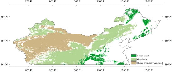
Figure 1.
Vegetation types in temperate China.
2.2. NDVI and Climate Dataset
GIMMS NDVI3G data derived from the Advanced Very-High-Resolution Radiometer (AVHRR) were used to extract spring phenology for the study area from 1982 to 2015. We used this dataset to study the impact of climate extremes on SOS because it has longer time coverage and includes the period of warming hiatus after 1997/98. The dataset was obtained using the maximum-value composite method with a temporal resolution of approximately 15 d and a spatial resolution of 1/12°. The data have undergone quality control (including atmospheric correction and orbital drift correction) [34] and are widely used for dynamic vegetation monitoring [35], land cover classification [36], and phenological information extraction [37,38] at regional and global scales.
The ERA-Interim dataset is used to calculate the CEIs, which is produced by the European Centre for Medium-Range Weather Forecasts. We chose to use ERA-Interim as our climate data source due to its widespread use and the fact that its spatial and temporal resolution met the requirements of our study. The spatial resolution of this dataset ranges from 0.125° to 2.5° [39,40]. We downloaded daily temperatures (including maximum and minimum temperatures) and precipitation at a spatial resolution of 0.125° for the years 1982–2015.
2.3. Methods
We extracted the SOS in temperate China based on the phenofit framework [41,42]. This framework contains six methods for fitting curves of NDVI, including asymmetric Gaussian [26] (AG hereafter), Beck’s [43] (Beck), Elmore’s [44] (Elmore), Gu’s [45] (Gu), Klosterman’s [46] (Klos), and Zhang’s [27] (Zhang), and four methods for determining phenological periods, including the threshold, derivative, Gu, and inflection methods. We used six curve-fitting methods combined with the derivative method to extract SOS. The NDVI curve-fitting functions for the six methods are shown in Table S1. The SOS corresponds to the time when the rate of change of the NDVI curve is locally maximized. To reduce uncertainty, we used an average of six methods to examine the impact of climate extremes on SOS.
The relationship between CEIs and SOS was examined using partial correlation analysis. We then used all-subsets regression to analyze the impact of CEIs on SOS. All-subsets regression tested all possible subsets of the set of potential independent variables and then used a specific criterion (e.g., adjusted R2) to determine the best model. There are 2k different subsets of the k possible independent variables that need to be tested. The equation below describes all possible regression models for the k variables:
where the first equation is a univariate model with i taking values from 1 to k, and the second equation is a bivariate model with i and j being unequal and taking values from 1 to k.
2.4. CEIs
The Expert Team (ET) of the CLIVAR project defines 27 core indices based on daily temperature and precipitation (http://etccdi.pacificclimate.org/list_27_indices.shtml, accessed on 1 September 2022). Some indices are based on fixed thresholds, and other thresholds are based on percentiles of the data series. We calculated 23 of these indices and calculated the mean daily maximum temperature and the mean daily minimum temperature. The CEIs were counted from 1 January to the SOS. Finally, we obtained 15 CEIs based on temperature and 10 based on precipitation. Table 1 shows the indices used in this study and their definitions.

Table 1.
Definition of climate extreme indices used in this study. TN, daily minimum temperature; TX, daily maximum temperature; RR, daily precipitation.
3. Results
3.1. Phenological Spatial Patterns
Using GIMMS NDVI3G data from 1982 to 2015, we obtained the spatial patterns of the SOS in temperate China calculated by six methods (Figure 2a–g). The area east of 105°E and south of 35°N is a low-latitude, low-altitude area, and the SOS of most pixels was less than 120 Julian days. In other regions, the SOS was relatively later, usually occurring after April. The Qinghai–Tibet Plateau has a lower latitude, but its high elevation caused its SOS to occur significantly later than that of the eastern region at the same latitude.
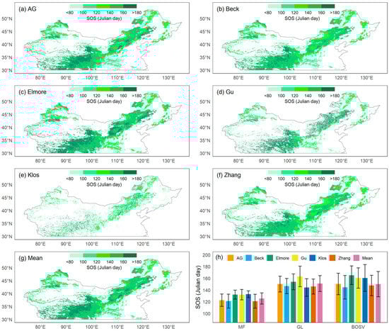
Figure 2.
Spatial patterns of the mean start of the growing season (SOS) from 1982 to 2015 using six methods: (a) asymmetric Gaussian method (AG), (b) Beck’s method (Beck), (c) Elmore’s method (Elmore), (d) Gu’s method (Gu), (e) Klosterman’s method (Klos), (f) Zhang’s method (Zhang), and (g) the mean of all methods (Mean). (h) The means and standard deviations of SOS for 1982–2015 estimated by six methods and their means for the three vegetation types: mixed forests (MF), grasslands (GL), and barren or sparsely vegetated land (BOSV).
On average, among the three vegetation types, the SOS of MF was the earliest (126 ± 10 d), while that of GL was the latest (151 ± 14 d). Spring phenology could not be detected in many pixels of BOSV because this vegetation type included desert areas in northwestern China. BOSV had the broadest range of SOS dates with standard deviations greater than 20 d.
3.2. Method Comparison
Similar spatial patterns were revealed by the SOS computed using the six different approaches, with the Klos method displaying the biggest divergence from the mean. For MF (Figure 2h), the SOS obtained using the Klos method had the highest mean and lowest standard deviation (133 ± 6 d), while the SOS values obtained using the Beck and Zhang methods had the lowest means and the highest standard deviations (121 ± 12 d). For GL, the SOS obtained using the Gu method had the highest mean and standard deviation (163 ± 18 d), while the SOS obtained by the Zhang method had the lowest mean and standard deviation (146 ± 13 d). For BOSV, the SOS obtained with the Elmore method had the highest mean and lowest standard deviation (165 ± 16 d), while the SOS obtained by the Beck method had the lowest mean (145 ± 20 d).
3.3. Temporal Dynamics of SOS and CEIs
To assess the influence of CEIs on the SOS, we examined trends in the SOS and CEIs. We first analyzed the average trend of the SOS obtained using the six methods. Overall, the SOS in the study area was significantly advanced at a rate of 0.97 days per decade between 1982 and 2015. Specifically, the SOS advanced in 63.9% of pixels, and in 23.4% of pixels the trends were significant (p < 0.05), while the SOS was delayed in 36.1% of pixels, and in 8.9% of pixels the trends were significant (Figure 3c). We observed that a significantly changed SOS occurred mainly in the eastern part of the study area. For the pixels with an advanced SOS, 90.7% of the changes were less than 0.8 days/year, and for the pixels with a delayed SOS, 81.5% of the changes were less than 0.6 days/year.
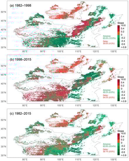
Figure 3.
Map of temporal trends of the start of the growing season (SOS) during (a) 1982–1998, (b) 1998–2015, and (c) 1982–2015. The insets show the pixels with p ≥ 0.05 (red) and p < 0.05 (green). Percentages indicate the proportion of pixels with advanced or delayed SOS (percentage of pixels with p value < 0.05 in parentheses).
However, the trend in the SOS was not consistent over time. Between 1982 and 1998, the SOS advanced in 63.4% of pixels, and in 12.0% of pixels the trends were significant (Figure 3a), while between 1998 and 2015 the SOS advanced in 46.0% of pixels, and in 6.0% of pixels the trends were significant (Figure 3b). The SOS was delayed in 36.6% of pixels during 1982–1998, and in 4.3% of pixels the trends were significant, while between 1998 and 2015 the SOS was delayed in 54.0% of pixels, and in 8.0% of pixels the trends were significant.
The direction and magnitude of the change in phenology were geographically variable and varied by vegetation type. Between 1982 and 2015, the SOS of most pixels for MF tended to be advanced, and the change was significant for more than half of the pixels (Table S2). For GL, more pixels had an advanced SOS than had a delayed SOS, and more pixels had a significantly advanced SOS than had a significantly delayed SOS—roughly 1.8 times more pixels had a significantly advanced SOS. For BOSV, the percentage of pixels with an advanced SOS was similar to that of pixels with a delayed SOS.
Interestingly, for all three vegetation types studied, the trend in the SOS changed over time and even reversed. For MF, the percentage of pixels with a significantly advanced SOS decreased from 21.9% in 1982–1998 to 8.4% in 1998–2015. For GL, during the period from 1982 to 1998, the percentage of pixels with a significantly advanced SOS was approximately twice that of pixels with a significantly delayed SOS. In contrast, during the period from 1998 to 2015, the percentage of pixels with a delayed SOS was higher than that of pixels with an advanced SOS. For BOSV, during the period from 1982 to 1998, the percentage of pixels with an advanced SOS was slightly higher than that with a delayed SOS. However, during the period from 1998 to 2015, the pixels with a significantly delayed SOS were approximately 3.5 times more significantly advanced.
We also investigated trends in CEIs over the period of 1982–2015 (Table S3). Overall, the extreme indices related to precipitation have no obvious trend (a similar percentage of significant increase or decrease), while some indices related to temperature have obvious trends. Between 1982 and 2015, the majority of pixel values of frost days (FD), cool nights (TN10P), min daily maximum temperature (TXN), and min daily minimum temperature (TNN) decreased, while the majority of pixel values of warm nights (TN90P), summer days (SU), and tropical nights (TR) increased.
However, the magnitude of change in the CEIs varies by vegetation type. For MF, over 60% of the pixels in FD show a significant decreasing trend, as do 28.9% of the pixels in max Tmin (TNX). Over 31% of the pixels in heavy precipitation days (R10MM) and total wet-day precipitation (PRCPTOT) show a significant decreasing trend. For GL, 24.2% of the pixels in FD show a significant decreasing trend, as do 17.3% of the pixels in TNN, while there is no significant trend in the extreme precipitation index. For BOSV, over 33% of the pixels in TN10P and ice days (ID) show a significant decreasing trend, and there is no significant trend in the extreme precipitation index.
To investigate the change in the trend of the CEIs over time, we calculated the difference in the percentage of the trend of the CEIs between 1998–2015 and 1982–1998 (Table S4). Overall, fewer pixels showed decreasing values for low-temperature-related indices (e.g., FD, TN10P, TX10P, CSDI, and ID), and fewer pixels showed increasing values for high-temperature-related indices (e.g., TN90P, TX90P, SU, and TR). For example, compared with 1982–1998, the percentage of pixels with decreasing FD decreased by 66% in 1998–2015, with the percentage of pixels showing a significant decreasing trend, decreasing from 18.6% to 1.0% (see Tables S5 and S6). For the extreme precipitation indices, the number of pixels with increasing values of wet-related indices (e.g., RX5DAY, R95P, R99P, CWD, R10MM, R20MM, and PRCPTOT) is decreasing, while the number of pixels with decreasing values of dry-related indices (CDD) is also decreasing.
The temporal trends of the CEIs vary by vegetation type. For MF, pixels with decreasing values of low-temperature-related indices (e.g., FD, TN10P, TX10P, CSDI, and ID) are decreasing, while there is no consistent temporal trend for high-temperature- and precipitation-related indices. The temporal trends of the CEIs for GL are similar to the overall temporal trends for the three vegetation types. For BOSV, most of the CEIs show the trend that the number of pixels with increasing values is increasing.
3.4. Correlation between SOS and CEIs
Considering the potential for correlation between CEIs, we calculated partial correlation coefficients between the CEIs and SOS (Figure 4). Overall, extreme temperatures were more strongly correlated with the SOS than extreme precipitation events during 1982–2015. For extreme temperature indices, the SOS was significantly positively correlated with FD (r = 0.83), TMINMEAN (r = 0.34), ID (r = 0.35), and TR (r = 0.36), while it was negatively correlated with TNN (r = −0.19) and SU (r = −0.17). For extreme precipitation indices, the SOS was significantly positively correlated with R95P (r = 0.14) and CDD (r = 0.15).
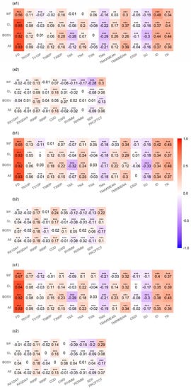
Figure 4.
Partial correlation coefficients between the start of the growing season (SOS) and climate extremes indices (CEIs) for mixed forests (MF), grasslands (GL), barren or sparsely vegetated land (BOSV), and all three vegetation types (All). Figures (a1,a2) are the partial correlation coefficients between the extreme temperature indices, extreme precipitation indices, and SOS from 1982 to 1998, respectively. Similarly, Figures (b1,b2,c1,c2) are the partial correlation coefficients between the extreme temperature indices, extreme precipitation indices, and SOS during 1998–2015 and 1982–2015, respectively. * p < 0.05, ** p < 0.01, *** p < 0.001.
The partial correlation coefficients between the SOS and the CEIs vary by vegetation type. For MF, the SOS was significantly positively correlated with FD (r = 0.67), TMINMEAN (r = 0.32), ID (r = 0.4), and TR (r = 0.37), while it was negatively correlated with TNN (r = −0.21). The SOS was significantly positively correlated with R95P (r = 0.11), CDD (r = 0.14), and PRCPTOT (r = 0.29), while it was negatively correlated with R20MM (r = −0.15) and SDII (r = −0.2). The partial correlation coefficients between the CEIs and SOS for GL are similar to those of all three vegetation types. For BOSV, the SOS was significantly positively correlated with FD (r = 0.82), ID (r = 0.38) and TR (r = 0.45), while it was negatively correlated with TXX (r = −0.29), TNN (r = −0.21), and SU (r = −0.3). The SOS was significantly positively correlated with R95P (r = 0.18), while it was negatively correlated with PRCPTOT (r = −0.17).
Comparing Figure 4(a1,b1,a2,b2), it can be found that the partial correlation coefficients between the extreme temperature indices, extreme precipitation indices, and SOS for 1982–1998 are similar to those for 1998–2015.
3.5. Comparing the Effects of CEIs on the SOS
Considering that the partial correlation coefficient reflects the degree of association between the two variables, its magnitude may not directly reflect the degree of influence of the CEIs on the SOS. We used all-subsets regression to select the best subsets from the predictor variables based on the adjusted R2 values (Figure 5). Overall, the regression model had the highest adjusted R2 of 0.93 when FD, TX90P, TNX, TNN, TMINMEAN, ID, TR, and R95P were used as predictor variables (Figure 5d). However, the predictor variables of the best regression models vary by vegetation type. For MF, when FD, TNX, TNN, TMINMEAN, ID, TR, CDD, R20MM, SDII, and PRCPTOT were used as predictor variables, the adjusted R2 of the regression model was highest, reaching 0.84. Similarly, for GL, when FD, TX90P, TNX, TNN, TMAXMEAN, TMINMEAN, SU, ID, TR, and R95P were used as predictor variables, the adjusted R2 of the regression model was the largest, reaching 0.93. For BOSV, FD, TN90P, TNN, TMINMEAN, SU, ID, and TR produced the highest adjusted R2 (0.96).

Figure 5.
Best subsets based on adjusted R2 for (a) mixed forests (MF), (b) grasslands (GL), (c) barren or sparsely vegetated land (BOSV), and (d) all three vegetation types (All).
To compare the regression coefficients, we eliminated the effects of the units of measurement of the variables on the coefficients and calculated the scaled coefficient. Table S7 lists the coefficients of the regression model. Overall, FD, TMINMEAN, TR, and ID affected the SOS of all three vegetation types, and FD and TMINMEAN had the greatest influence. For MF, the SOS was most affected by TMINMEAN, while for GL and BOSV the SOS was most affected by FD. These results indicate that the SOS of the three vegetation types was most affected by extreme temperature events. In addition, extreme precipitation events (e.g., SDII and R20MM) also affected the SOS of MF.
4. Discussion
4.1. Temporal Trends in SOS
Previous studies have shown that for most of temperate China there was no significant trend in vegetation spring phenology from 1982 to 2006 [38], which is consistent with the findings of the present study. Approximately half (50.3%) of the pixels of temperate ecosystems in China had an advancing trend from 1999 to 2013 [47], and our results showed that 46% of the pixels of temperate vegetation in China had an advancing trend from 1998 to 2015. The reason for this difference may be the satellite data used and the difference in the study period.
Similar to the findings of this study, Cong et al. demonstrated that the spring phenology of temperate vegetation in China advanced at an average rate of 1.3 ± 0.6 days from 1982 to 2010 [48]. Our study showed that most pixels of the SOS for the three vegetation types from 1982 to 2015 showed an advancing trend; however, this trend was not consistent throughout the study period. Studies have shown that the SOS in temperate vegetation in China mainly showed an advancement trend in the 1980s and early 1990s, with the turning point occurring in the mid-to-late 1990s [38], and similar conclusions can be drawn from our analysis. The SOS of all three vegetation types showed a trend from advancing to delayed, especially for GL and BOSV. For MF, most pixels of the SOS from 1998 to 2015 showed an advancement trend; however, the percentage of pixels with an advancement trend decreased significantly compared to 1982–1998. The findings of this study demonstrated that, although the trend was not significant for the majority of pixels (p > 0.05), the SOS of temperate vegetation in China primarily had a delayed trend between 1998 and 2015.
4.2. Temporal Trends in CEIs
Climate change is highly geographic and seasonal in nature [49,50]. For instance, over longer periods of time, global temperatures have shown significant warming tendencies in all seasons other than winter, whereas significant cooling trends are observed in winter across much of eastern North America and northern Eurasia [51]. The frequency of extreme climate occurrences has noticeably changed as global warming continues. Studies have shown that the increase in daily minimum temperature is more pronounced than the increase in daily maximum temperature [21]. During 1961–2015, indices related to high temperatures (e.g., tropical nights, summer days, warm days, and warm nights) showed an overall increasing trend in China, while indices related to low temperatures (e.g., frost days, ice days, and cool nights) showed a decreasing trend [52]. This is comparable to the findings of this study, despite the differences in study time and index calculation. In general, our results show no significant trend of increasing or decreasing extreme precipitation indices. This lack of a general trend may be due to the regional and seasonal nature of precipitation. The temporal trend of global warming is not uniform, and it experienced a hiatus of more than a decade after the 1997/98 El Niño event [50,53]. The study points out that the average temperature in China decreased by 0.221 °C per decade during 1998–2012, compared with an increase of 0.427 °C per decade during 1960–1998 [54]. The disruption of warming is reflected not only in the average temperature but also in extreme climate events. For instance, a warming hiatus occurred in eastern China during the 20 years after 1997, marked by a significant decline in daily minimum temperatures [55]. The trend differences in CEIs between the periods of 1982–1998 and 1998–2015 in this study may be explained by the warming hiatus.
4.3. Responses of SOS to CEIs
Although precipitation can change how sensitive vegetation spring phenology is to temperature, it has been demonstrated that temperature and not precipitation more closely correlates with vegetation spring phenology [48]. Our findings demonstrated that the extreme temperature indices had a higher correlation with the vegetation SOS than did the extreme precipitation indices. Of all the CEIs studied, frost days had the highest correlation with the vegetation SOS, and all-subsets regression showed that frost days also had a very strong influence on spring phenology. Currently, growing degree days (GDD) are often seen as the dominant factor driving spring phenology. A growing degree day refers to the part where the temperature exceeds a certain threshold (commonly set at 0 or 5 °C) [56]. The growing season begins when the cumulative GDD exceed a specific threshold. In addition, day length may also affect spring phenology [12,13]. Recent research has revealed that spring frost frequency drives the initiation of budburst, despite the fact that GDD can act quickly once the growing season has started [57]. This may be because the leaf-out is regulated by a strategy to minimize frost damage [58].
The timing of phenology reflects the trade-off between maximizing resource acquisition and avoiding frost damage [12,59,60,61]. Plants have two coping strategies when faced with undesirable conditions: evolving frost-resistant tissues to increase tolerance or avoiding frost damage with seeds or underground stems or regenerating roots, an example being the defoliation strategy of many woody plants [60,62]. Prebudburst frosts usually only delay budburst, but if vegetation experiences higher temperatures in early spring and budbursts occur early, experiencing subsequent frost may harm the plants and thus affect ecosystem composition and productivity [63]. Different species have separate growth strategies, tolerances, and resilience, resulting in various levels of impact. For example, conservative growth strategies render yellow birch and American beech largely unaffected by late spring frosts, while sugar maple suffers from frost damage, resulting in leaf loss and delayed crown development [64]. In addition, European beech showed low resistance to late frost events but high resilience in radial growth [65]. Considering the trend of increasing frost area in recent years, the effects of frost need to be continuously monitored, especially the damage from frost after the beginning of the growing season.
Studies have shown that the impacts of daytime and nighttime temperatures on vegetation spring phenology vary significantly, with Northern Hemisphere spring phenology being driven primarily by daytime temperatures [56]. According to our findings, spring phenology is more sensitive to TMINMEAN than TMAXMEAN. There may be several reasons behind this phenomenon. First of all, the effects of daytime and nighttime temperatures may vary with the seasons. For example, studies have shown that spring phenology in the temperate grasslands of China is mainly influenced by daytime temperatures in winter and by nighttime temperatures in spring [66]. On the other hand, the asymmetric effects of temperature on spring phenology may be spatially heterogeneous. For example, nighttime temperatures have a higher impact on spring phenology on the Tibetan Plateau than daytime temperatures [67]. In addition, previous studies have typically used the preseason approach, i.e., the months with the largest partial correlation coefficient between spring phenology and the temperature indicators before spring phenology were defined as preseason, which may lead to inconsistent time periods for daytime temperature and nighttime temperature statistics, whereas the time periods for statistical extreme climate indices are consistent in this study.
Phenology models are important tools for predicting phenological changes and are based on an understanding of the environmental factors influencing vegetation phenology. Temperature-based spring phenology models usually assume that plants need to undergo two processes: accumulating chilling temperature and accumulating forcing temperature [68]. Some models suggest that plants need to accumulate a specific amount of chilling temperature in winter to break dormancy, after which they begin to accumulate forcing temperature until the thermal requirements are met, while others suggest that the two processes are not sequential and there is an interaction between the chilling requirements and the forcing requirements [69,70,71]. In extremely warm years, the relationship between chilling requirements and forcing requirements may be altered. It has been shown that white ash trees have higher forcing requirements in extreme warm years than in nonextreme years, which can constrain the advancement of leaf-out and ultimately lead to early leaf-out predicted by existing phenology models [10]. Whether this phenomenon occurs for other species and the magnitude of the effect require further study.
Overall, the partial correlation coefficients between the SOS and extreme precipitation indices were low, with PRCPTOT having an opposite effect on the SOS for MF and BOSV. This may be because BOSV is mainly distributed in desert areas, whereas MF is mainly distributed in areas with better precipitation conditions. Different soil water contents and drought indices (annual precipitation divided by potential evapotranspiration) may contribute to the differences in the effects of precipitation events on vegetation phenology [72]. Forests tend to be less constrained by moisture conditions, while deserts have lower soil water content, making plants vulnerable to precipitation events. Pregrowing season precipitation has different effects on different vegetation types, and for moisture-limited areas, increased cumulative precipitation usually leads to an earlier vegetation SOS [25]. Our results suggest that extreme precipitation events may have an opposite effect to cumulative precipitation (e.g., R95P vs. PRCPTOT for BOSV), and similar findings have been reported in previous studies [73].
4.4. Limitations and Uncertainties
The findings of this study indicate that at the end of the 20th century the trend of advancing spring phenology in temperate China reversed. However, it is worth noting that different satellite data may yield inconsistent results. A typical controversy is the trend of the spring phenology of vegetation on the TP after 2000. Using the AVHRR dataset, Yu et al. analyzed the TP’s spring phenology of vegetation and found that the SOS had two distinct trends: a slow advancing trend from the early 1980s to the mid-1990s, and a rapid delay trend from the mid-1990s to 2006 [74]. However, a study by Zhang et al. based on AVHRR, SPOT, and MODIS data showed a consistent advancement trend in the spring phenology of the TP from 1982 to 2011 [75]. Ding et al. extracted the SOS of the TP using SPOT data, and the results showed that the SOS was delayed and then advanced from 1999 to 2009, with an overall advancing trend [76]. In addition, a study based on tree-ring data showed that spring phenology on the TP was significantly advanced from 2000 to 2009, while there was a trend of advancement that was not significant from 2000 to 2011 [77]. In a recent study combining AVHRR, MODIS, and aboveground biomass datasets to analyze vegetation growth on the TP, it was found that AVHRR NDVI did not capture an advancing trend in vegetation growth from 2000 to 2014, while MODIS NDVI partially captured this trend, and that all satellite-derived NDVI understated the advance in plant growth [78]. In summary, it is clear that the data sources and the study period may have important effects on the results. Therefore, when using satellite data to analyze vegetation phenology, the results from multiple data sources, especially ground-based observations, need to be combined [79].
5. Conclusions
Our study shows that the SOS was significantly advanced, with an average rate of 0.97 days per decade, and there was no consistent trend in either the SOS or CEIs from 1982 to 2015, with the turning point occurring in the late 1990s. The SOS of the three vegetation types studied showed mainly an advancement trend in 1982–1998 and a delayed trend or significant decrease in pixels with an advancement trend in 1998–2015. Overall, some of the extreme temperature indices have a clear trend, while the extreme precipitation indices do not have a clear trend, although they are affected by a warming hiatus after 1997/98. Extreme temperature showed a stronger correlation with the SOS than extreme precipitation. FD, TMINMEAN, TR, and ID all affected the SOS of the three vegetation types, of which FD and TMINMEAN showed the strongest effects. For MF, the SOS was most affected by TMINMEAN, while for GL and BOSV the SOS was most affected by FD. Considering the geographical, seasonal, and destructive nature of extreme climate events, their impact on terrestrial ecosystems requires continuous attention. In addition, we suggest integrating multiple data sources to investigate the changes in vegetation phenology, especially ground-based observations.
Supplementary Materials
The following are available online at https://www.mdpi.com/article/10.3390/rs15030686/s1, Table S1: Summary of six curve fitting methods in determining start of the growing season (SOS) from satellite-derived NDVI data. Table S2: Temporal trends of the start of the growing season (SOS) for the three vegetation types: mixed forest (MF), grasslands (GL), and barren or sparsely vegetated land (BOSV). The percentages represent the percentage of pixels with advanced or delayed SOS (percentage of pixels with p value < 0.05 in parentheses). Table S3: Changes in climate extremes indices over the period 1982–2015. Negative means that the climate extremes indices decrease with the year (percentage of pixels with p < 0.05 in parentheses), while positive means that it increases with the year. The values in the table are the percentage of the trend. Table S4: Changes in trends in climate extremes indices from 1982–1998 to 1998–2015. Negative means that the climate extremes indices decrease with the year (percentage of pixels with p < 0.05 in parentheses), while positive means that it increases with the year. The values in the table are the difference in the percentage of the trend in the climate extremes indices between 1998-2015 and 1982–1998. Table S5: Changes in extreme climate indices over the period 1982–1998. Negative means that the extreme climate indices decreases with the year (percentage of pixels with p < 0.05 in parentheses), while positive means that it increases with the year. The values in the table are the percentage of the trend. Table S6: Changes in extreme climate indices over the period 1998–2015. Negative means that the extreme climate indices decreases with the year (percentage of pixels with p < 0.05 in parentheses), while positive means that it increases with the year. The values in the table are the percentage of the trend. Table S7: Regression coefficients for the best regression model of climate extremes indices and the start of the growing season (SOS) for three vegetation types: mixed forest (MF), grasslands (GL), and barren or sparsely vegetated land (BOSV).
Author Contributions
Conceptualization, Y.F.; methodology, Y.M., X.Z., and Y.F.; software, validation, formal analysis, and data curation, Y.M.; investigation, Y.F. and X.Z.; writing—original draft, Y.F. and Y.M.; writing—review and editing, Y.M., Z.L., and J.Z.; visualization, Y.M.; funding acquisition, Y.F. and F.H.; supervision, Y.F., J.Z., and F.H. All authors have read and agreed to the published version of the manuscript.
Funding
This study was funded by the International Cooperation and Exchanges NSFC-FWO (32111530083), the National Science Fund for Distinguished Young Scholars (Grant No. 42025101), the National Natural Science Foundation of China (Grant No. 31770516), and the 111 Project (Grant No. B18006).
Data Availability Statement
Land cover data are available online at https://lpdaac.usgs.gov/products/mcd12q1v006/. Climate data can be found at https://apps.ecmwf.int/datasets/data/interim-full-daily/levtype=sfc/. GIMMS NDVI data are available online at http://poles.tpdc.ac.cn/en/data/9775f2b4-7370-4e5e-a537-3482c9a83d88/ (accessed on 1 March 2022).
Conflicts of Interest
The authors declare no conflict of interest.
References
- Urry, J. Climate change and society. In Why the Social Sciences Matter; Springer: Cham, Switzerland, 2015; pp. 45–59. [Google Scholar]
- Anderson, R.; Bayer, P.E.; Edwards, D. Climate change and the need for agricultural adaptation. Curr. Opin. Plant Biol. 2020, 56, 197–202. [Google Scholar] [CrossRef]
- Salimi, M.; Al-Ghamdi, S.G. Climate change impacts on critical urban infrastructure and urban resiliency strategies for the Middle East. Sustain. Cities Soc. 2020, 54, 101948. [Google Scholar] [CrossRef]
- Gernaat, D.E.; de Boer, H.S.; Daioglou, V.; Yalew, S.G.; Müller, C.; van Vuuren, D.P. Climate change impacts on renewable energy supply. Nat. Clim. Chang. 2021, 11, 119–125. [Google Scholar] [CrossRef]
- Richardson, A.D.; Keenan, T.F.; Migliavacca, M.; Ryu, Y.; Sonnentag, O.; Toomey, M. Climate change, phenology, and phenological control of vegetation feedbacks to the climate system. Agric. For. Meteorol. 2013, 169, 156–173. [Google Scholar] [CrossRef]
- Cleland, E.E.; Chuine, I.; Menzel, A.; Mooney, H.A.; Schwartz, M.D. Shifting plant phenology in response to global change. Trends Ecol. Evol. 2007, 22, 357–365. [Google Scholar] [CrossRef]
- Piao, S.; Liu, Q.; Chen, A.; Janssens, I.A.; Fu, Y.; Dai, J.; Liu, L.; Lian, X.; Shen, M.; Zhu, X. Plant phenology and global climate change: Current progresses and challenges. Glob. Chang. Biol. 2019, 25, 1922–1940. [Google Scholar] [CrossRef] [PubMed]
- Suttle, K.; Thomsen, M.A.; Power, M.E. Species interactions reverse grassland responses to changing climate. Science 2007, 315, 640–642. [Google Scholar] [CrossRef]
- Richardson, A.D.; Andy Black, T.; Ciais, P.; Delbart, N.; Friedl, M.A.; Gobron, N.; Hollinger, D.Y.; Kutsch, W.L.; Longdoz, B.; Luyssaert, S. Influence of spring and autumn phenological transitions on forest ecosystem productivity. Philos. Trans. R. Soc. Lond. Ser. B 2010, 365, 3227–3246. [Google Scholar] [CrossRef]
- Carter, J.M.; Orive, M.E.; Gerhart, L.M.; Stern, J.H.; Marchin, R.M.; Nagel, J.; Ward, J.K. Warmest extreme year in US history alters thermal requirements for tree phenology. Oecologia 2017, 183, 1197–1210. [Google Scholar] [CrossRef]
- Geng, X.; Fu, Y.H.; Hao, F.; Zhou, X.; Zhang, X.; Yin, G.; Vitasse, Y.; Piao, S.; Niu, K.; De Boeck, H.J. Climate warming increases spring phenological differences among temperate trees. Glob. Chang. Biol. 2020, 26, 5979–5987. [Google Scholar] [CrossRef]
- Fu, Y.H.; Zhang, X.; Piao, S.; Hao, F.; Geng, X.; Vitasse, Y.; Zohner, C.; Peñuelas, J.; Janssens, I.A. Daylength helps temperate deciduous trees to leaf-out at the optimal time. Glob. Chang. Biol. 2019, 25, 2410–2418. [Google Scholar] [CrossRef] [PubMed]
- Fu, Y.H.; Piao, S.; Zhou, X.; Geng, X.; Hao, F.; Vitasse, Y.; Janssens, I.A. Short photoperiod reduces the temperature sensitivity of leaf-out in saplings of Fagus sylvatica but not in horse chestnut. Glob. Chang. Biol. 2019, 25, 1696–1703. [Google Scholar] [CrossRef] [PubMed]
- De Reaumur, R. Observations du thermomètre faites à Paris pendant l’année 1735, comparées avec celles qui ont été faites sous la ligne, à l’Isle de France, à Alger et quelques unes de nos iles de l’Amérique. Mémoires l’Académie R des Sci. 1735, 1735, 545–576. [Google Scholar]
- Masle, J.; Doussinault, G.; Farquhar, G.; Sun, B. Foliar stage in wheat correlates better to photothermal time than to thermal time. Plant Cell Environ. 1989, 12, 235–247. [Google Scholar] [CrossRef]
- Jentsch, A.; Kreyling, J.; Boettcher-Treschkow, J.; Beierkuhnlein, C. Beyond gradual warming: Extreme weather events alter flower phenology of European grassland and heath species. Glob. Chang. Biol. 2009, 15, 837–849. [Google Scholar] [CrossRef]
- Li, P.; Liu, Z.; Zhou, X.; Xie, B.; Li, Z.; Luo, Y.; Zhu, Q.; Peng, C. Combined control of multiple extreme climate stressors on autumn vegetation phenology on the Tibetan Plateau under past and future climate change. Agric. For. Meteorol. 2021, 308, 108571. [Google Scholar] [CrossRef]
- Du, J.; Li, K.; He, Z.; Chen, L.; Lin, P.; Zhu, X. Daily minimum temperature and precipitation control on spring phenology in arid-mountain ecosystems in China. Int. J. Climatol. 2020, 40, 2568–2579. [Google Scholar] [CrossRef]
- Deng, H.; Yin, Y.; Wu, S.; Xu, X. Contrasting drought impacts on the start of phenological growing season in Northern China during 1982–2015. Int. J. Climatol. 2020, 40, 3330–3347. [Google Scholar] [CrossRef]
- Masson-Delmotte, V.; Zhai, P.; Pirani, A.; Connors, S.L.; Péan, C.; Berger, S.; Caud, N.; Chen, Y.; Goldfarb, L.; Gomis, M.I. Climate Change 2021: The Physical Science Basis. Contribution of Working Group I to the Sixth Assessment Report of the Intergovernmental Panel on Climate Change; IPCC: Geneva, Switzerland, 2021. [Google Scholar]
- Wang, H.-J.; Sun, J.-Q.; Chen, H.-P.; Zhu, Y.-L.; Zhang, Y.; Jiang, D.-B.; Lang, X.-M.; Fan, K.; Yu, E.-T.; Yang, S. Extreme climate in China: Facts, simulation and projection. Meteorol. Z. 2012, 21, 279. [Google Scholar] [CrossRef]
- Guan, J.; Yao, J.; Li, M.; Li, D.; Zheng, J. Historical changes and projected trends of extreme climate events in Xinjiang, China. Clim. Dyn. 2022, 59, 1753–1774. [Google Scholar] [CrossRef]
- Shi, J.; Cui, L.; Wen, K.; Tian, Z.; Wei, P.; Zhang, B. Trends in the consecutive days of temperature and precipitation extremes in China during 1961–2015. Environ. Res. 2018, 161, 381–391. [Google Scholar] [CrossRef]
- Wu, X.; Hao, Z.; Hao, F.; Zhang, X. Variations of compound precipitation and temperature extremes in China during 1961–2014. Sci. Total Environ. 2019, 663, 731–737. [Google Scholar] [CrossRef]
- Piao, S.; Fang, J.; Zhou, L.; Ciais, P.; Zhu, B. Variations in satellite-derived phenology in China’s temperate vegetation. Glob. Chang. Biol. 2006, 12, 672–685. [Google Scholar] [CrossRef]
- Jonsson, P.; Eklundh, L. Seasonality extraction by function fitting to time-series of satellite sensor data. IEEE Trans. Geosci. Remote Sens. 2002, 40, 1824–1832. [Google Scholar] [CrossRef]
- Zhang, X.; Friedl, M.A.; Schaaf, C.B.; Strahler, A.H.; Hodges, J.C.; Gao, F.; Reed, B.C.; Huete, A. Monitoring vegetation phenology using MODIS. Remote Sens. Environ. 2003, 84, 471–475. [Google Scholar] [CrossRef]
- Cong, N.; Piao, S.; Chen, A.; Wang, X.; Lin, X.; Chen, S.; Han, S.; Zhou, G.; Zhang, X. Spring vegetation green-up date in China inferred from SPOT NDVI data: A multiple model analysis. Agric. For. Meteorol. 2012, 165, 104–113. [Google Scholar] [CrossRef]
- White, M.A.; de Beurs, K.M.; Didan, K.; Inouye, D.W.; Richardson, A.D.; Jensen, O.P.; O’keefe, J.; Zhang, G.; Nemani, R.R.; van Leeuwen, W.J. Intercomparison, interpretation, and assessment of spring phenology in North America estimated from remote sensing for 1982–2006. Glob. Chang. Biol. 2009, 15, 2335–2359. [Google Scholar] [CrossRef]
- Liu, Q.; Fu, Y.H.; Zeng, Z.; Huang, M.; Li, X.; Piao, S. Temperature, precipitation, and insolation effects on autumn vegetation phenology in temperate China. Glob. Chang. Biol. 2016, 22, 644–655. [Google Scholar] [CrossRef]
- Zhou, X.; Geng, X.; Yin, G.; Hänninen, H.; Hao, F.; Zhang, X.; Fu, Y.H. Legacy effect of spring phenology on vegetation growth in temperate China. Agric. For. Meteorol. 2020, 281, 107845. [Google Scholar] [CrossRef]
- Channan, S.; Collins, K.; Emanuel, W. Global Mosaics of the Standard MODIS Land Cover Type Data; University of Maryland and the Pacific Northwest National Laboratory: College Park, ML, USA, 2014; Volume 30. [Google Scholar]
- Friedl, M.A.; Sulla-Menashe, D.; Tan, B.; Schneider, A.; Ramankutty, N.; Sibley, A.; Huang, X. MODIS Collection 5 global land cover: Algorithm refinements and characterization of new datasets. Remote Sens. Environ. 2010, 114, 168–182. [Google Scholar] [CrossRef]
- Pinzon, J.E.; Tucker, C.J. A non-stationary 1981–2012 AVHRR NDVI3g time series. Remote Sens. 2014, 6, 6929–6960. [Google Scholar] [CrossRef]
- Detsch, F.; Otte, I.; Appelhans, T.; Hemp, A.; Nauss, T. Seasonal and long-term vegetation dynamics from 1-km GIMMS-based NDVI time series at Mt. Kilimanjaro, Tanzania. Remote Sens. Environ. 2016, 178, 70–83. [Google Scholar] [CrossRef]
- He, Y.; Lee, E.; Warner, T.A. A time series of annual land use and land cover maps of China from 1982 to 2013 generated using AVHRR GIMMS NDVI3g data. Remote Sens. Environ. 2017, 199, 201–217. [Google Scholar] [CrossRef]
- Mo, Y.; Chen, S.; Jin, J.; Lu, X.; Jiang, H. Temporal and spatial dynamics of phenology along the North–South Transect of Northeast Asia. Int. J. Remote Sens. 2019, 40, 7922–7940. [Google Scholar] [CrossRef]
- Wu, X.; Liu, H. Consistent shifts in spring vegetation green-up date across temperate biomes in China, 1982–2006. Glob. Chang. Biol. 2013, 19, 870–880. [Google Scholar] [CrossRef]
- Berrisford, P.; Dee, D.; Fielding, K.; Fuentes, M.; Kallberg, P.; Kobayashi, S.; Uppala, S. The ERA-Interim Archive; ERA report series; ECMWF: Reading, UK, 2009; pp. 1–16. [Google Scholar]
- Berrisford, P.; Dee, D.; Poli, P.; Brugge, R.; Simmons, A. The ERA-Interim archive, version 2.0. Nihon Seirigaku Zasshi J. Physiol. Soc. Jpn. 2011, 31, 1–40. [Google Scholar]
- Kong, D.; Xiao, M.; Zhang, Y.; Gu, X.; Cui, J. phenofit: Extract remote sensing vegetation phenology. Zenodo 2020. [Google Scholar] [CrossRef]
- Zhang, Q.; Kong, D.; Shi, P.; Singh, V.P.; Sun, P. Vegetation phenology on the Qinghai-Tibetan Plateau and its response to climate change (1982–2013). Agric. For. Meteorol. 2018, 248, 408–417. [Google Scholar] [CrossRef]
- Beck, P.S.; Atzberger, C.; Høgda, K.A.; Johansen, B.; Skidmore, A.K. Improved monitoring of vegetation dynamics at very high latitudes: A new method using MODIS NDVI. Remote Sens. Environ. 2006, 100, 321–334. [Google Scholar] [CrossRef]
- Elmore, A.J.; Guinn, S.M.; Minsley, B.J.; Richardson, A.D. Landscape controls on the timing of spring, autumn, and growing season length in mid-A tlantic forests. Glob. Chang. Biol. 2012, 18, 656–674. [Google Scholar] [CrossRef]
- Gu, L.; Post, W.M.; Baldocchi, D.D.; Black, T.A.; Suyker, A.E.; Verma, S.B.; Vesala, T.; Wofsy, S.C. Characterizing the seasonal dynamics of plant community photosynthesis across a range of vegetation types. In Phenology of Ecosystem Processes; Springer: Cham, Switzerland, 2009; pp. 35–58. [Google Scholar]
- Klosterman, S.; Hufkens, K.; Gray, J.; Melaas, E.; Sonnentag, O.; Lavine, I.; Mitchell, L.; Norman, R.; Friedl, M.; Richardson, A. Evaluating remote sensing of deciduous forest phenology at multiple spatial scales using PhenoCam imagery. Biogeosciences 2014, 11, 4305–4320. [Google Scholar] [CrossRef]
- Wu, C.; Hou, X.; Peng, D.; Gonsamo, A.; Xu, S. Land surface phenology of China’s temperate ecosystems over 1999–2013: Spatial–temporal patterns, interaction effects, covariation with climate and implications for productivity. Agric. For. Meteorol. 2016, 216, 177–187. [Google Scholar] [CrossRef]
- Cong, N.; Wang, T.; Nan, H.; Ma, Y.; Wang, X.; Myneni, R.B.; Piao, S. Changes in satellite-derived spring vegetation green-up date and its linkage to climate in China from 1982 to 2010: A multimethod analysis. Glob. Chang. Biol. 2013, 19, 881–891. [Google Scholar] [CrossRef] [PubMed]
- Zhai, P.; Zhang, X.; Wan, H.; Pan, X. Trends in total precipitation and frequency of daily precipitation extremes over China. J. Clim. 2005, 18, 1096–1108. [Google Scholar] [CrossRef]
- Wang, L.; Yuan, X.; Xie, Z.; Wu, P.; Li, Y. Increasing flash droughts over China during the recent global warming hiatus. Sci. Rep. 2016, 6, 30571. [Google Scholar] [CrossRef]
- Cohen, J.L.; Furtado, J.C.; Barlow, M.; Alexeev, V.A.; Cherry, J.E. Asymmetric seasonal temperature trends. Geophys. Res. Lett. 2012, 39, L04705. [Google Scholar] [CrossRef]
- Shi, J.; Cui, L.; Ma, Y.; Du, H.; Wen, K. Trends in temperature extremes and their association with circulation patterns in China during 1961–2015. Atmos. Res. 2018, 212, 259–272. [Google Scholar] [CrossRef]
- Meehl, G.A.; Arblaster, J.M.; Fasullo, J.T.; Hu, A.; Trenberth, K.E. Model-based evidence of deep-ocean heat uptake during surface-temperature hiatus periods. Nat. Clim. Change 2011, 1, 360–364. [Google Scholar] [CrossRef]
- Du, Q.; Zhang, M.; Wang, S.; Che, C.; Ma, R.; Ma, Z. Changes in air temperature over China in response to the recent global warming hiatus. J. Geog. Sci. 2019, 29, 496–516. [Google Scholar] [CrossRef]
- Chen, Y.; Zhai, P. Persisting and strong warming hiatus over eastern China during the past two decades. Environ. Res. Lett. 2017, 12, 104010. [Google Scholar] [CrossRef]
- Piao, S.; Tan, J.; Chen, A.; Fu, Y.H.; Ciais, P.; Liu, Q.; Janssens, I.A.; Vicca, S.; Zeng, Z.; Jeong, S.-J. Leaf onset in the northern hemisphere triggered by daytime temperature. Nat. Commun. 2015, 6, 6911. [Google Scholar] [CrossRef] [PubMed]
- Marquis, B.; Bergeron, Y.; Simard, M.; Tremblay, F. Probability of spring frosts, not growing degree-days, drives onset of spruce bud burst in plantations at the boreal-temperate forest ecotone. Front. Plant Sci. 2020, 11, 1031. [Google Scholar] [CrossRef] [PubMed]
- Lenz, A.; Hoch, G.; Körner, C.; Vitasse, Y. Convergence of leaf-out towards minimum risk of freezing damage in temperate trees. Funct. Ecol. 2016, 30, 1480–1490. [Google Scholar] [CrossRef]
- Saxe, H.; Cannell, M.G.; Johnsen, Ø.; Ryan, M.G.; Vourlitis, G. Tree and forest functioning in response to global warming. New Phytol. 2001, 149, 369–399. [Google Scholar] [CrossRef] [PubMed]
- Kreyling, J. Winter climate change: A critical factor for temperate vegetation performance. Ecology 2010, 91, 1939–1948. [Google Scholar] [CrossRef]
- Fisichelli, N.; Vor, T.; Ammer, C. Broadleaf seedling responses to warmer temperatures “chilled” by late frost that favors conifers. Eur. J. For. Res. 2014, 133, 587–596. [Google Scholar] [CrossRef]
- Chamberlain, C.J.; Cook, B.I.; García de Cortázar-Atauri, I.; Wolkovich, E.M. Rethinking false spring risk. Glob. Chang. Biol. 2019, 25, 2209–2220. [Google Scholar] [CrossRef] [PubMed]
- Gu, L.; Hanson, P.J.; Post, W.M.; Kaiser, D.P.; Yang, B.; Nemani, R.; Pallardy, S.G.; Meyers, T. The 2007 eastern US spring freeze: Increased cold damage in a warming world? BioScience 2008, 58, 253–262. [Google Scholar] [CrossRef]
- Hufkens, K.; Friedl, M.A.; Keenan, T.F.; Sonnentag, O.; Bailey, A.; O’Keefe, J.; Richardson, A.D. Ecological impacts of a widespread frost event following early spring leaf-out. Glob. Chang. Biol. 2012, 18, 2365–2377. [Google Scholar] [CrossRef]
- Príncipe, A.; van der Maaten, E.; van der Maaten-Theunissen, M.; Struwe, T.; Wilmking, M.; Kreyling, J. Low resistance but high resilience in growth of a major deciduous forest tree (Fagus sylvatica L.) in response to late spring frost in southern Germany. Trees 2017, 31, 743–751. [Google Scholar] [CrossRef]
- Shen, X.; Liu, B.; Henderson, M.; Wang, L.; Wu, Z.; Wu, H.; Jiang, M.; Lu, X. Asymmetric effects of daytime and nighttime warming on spring phenology in the temperate grasslands of China. Agric. For. Meteorol. 2018, 259, 240–249. [Google Scholar] [CrossRef]
- Shen, M.; Piao, S.; Chen, X.; An, S.; Fu, Y.H.; Wang, S.; Cong, N.; Janssens, I.A. Strong impacts of daily minimum temperature on the green-up date and summer greenness of the Tibetan Plateau. Glob. Chang. Biol. 2016, 22, 3057–3066. [Google Scholar] [CrossRef] [PubMed]
- Hänninen, H.; Kramer, K.; Tanino, K.; Zhang, R.; Wu, J.; Fu, Y.H. Experiments are necessary in process-based tree phenology modelling. Trends Plant Sci. 2019, 24, 199–209. [Google Scholar] [CrossRef] [PubMed]
- Hänninen, H. Modelling bud dormancy release in trees from cool and temperate regions. Acta For. Fenn. 1990, 213, 7660. [Google Scholar] [CrossRef]
- Kramer, K. Selecting a model to predict the onset of growth of Fagus sylvatica. J. Appl. Ecol. 1994, 31, 172–181. [Google Scholar] [CrossRef]
- Cesaraccio, C.; Spano, D.; Snyder, R.L.; Duce, P. Chilling and forcing model to predict bud-burst of crop and forest species. Agric. For. Meteorol. 2004, 126, 1–13. [Google Scholar] [CrossRef]
- Zeppel, M.; Wilks, J.V.; Lewis, J.D. Impacts of extreme precipitation and seasonal changes in precipitation on plants. Biogeosciences 2014, 11, 3083–3093. [Google Scholar] [CrossRef]
- Qiu, T.; Song, C.; Clark, J.S.; Seyednasrollah, B.; Rathnayaka, N.; Li, J. Understanding the continuous phenological development at daily time step with a bayesian hierarchical space-time model: Impacts of climate change and extreme weather events. Remote Sens. Environ. 2020, 247, 111956. [Google Scholar] [CrossRef]
- Yu, H.; Luedeling, E.; Xu, J. Winter and spring warming result in delayed spring phenology on the Tibetan Plateau. Proc. Natl. Acad. Sci. USA 2010, 107, 22151–22156. [Google Scholar] [CrossRef]
- Zhang, G.; Zhang, Y.; Dong, J.; Xiao, X. Green-up dates in the Tibetan Plateau have continuously advanced from 1982 to 2011. Proc. Natl. Acad. Sci. USA 2013, 110, 4309–4314. [Google Scholar] [CrossRef]
- Ding, M.; Zhang, Y.; Sun, X.; Liu, L.; Wang, Z.; Bai, W. Spatiotemporal variation in alpine grassland phenology in the Qinghai-Tibetan Plateau from 1999 to 2009. Chin. Sci. Bull. 2013, 58, 396–405. [Google Scholar] [CrossRef]
- Yang, B.; He, M.; Shishov, V.; Tychkov, I.; Vaganov, E.; Rossi, S.; Ljungqvist, F.C.; Bräuning, A.; Grießinger, J. New perspective on spring vegetation phenology and global climate change based on Tibetan Plateau tree-ring data. Proc. Natl. Acad. Sci. USA 2017, 114, 6966–6971. [Google Scholar] [CrossRef] [PubMed]
- Wang, H.; Liu, H.; Huang, N.; Bi, J.; Ma, X.; Ma, Z.; Shangguan, Z.; Zhao, H.; Feng, Q.; Liang, T. Satellite-derived NDVI underestimates the advancement of alpine vegetation growth over the past three decades. Ecology 2021, 102, E03518. [Google Scholar] [CrossRef] [PubMed]
- Fu, Y.H.; Piao, S.; Op de Beeck, M.; Cong, N.; Zhao, H.; Zhang, Y.; Menzel, A.; Janssens, I.A. Recent spring phenology shifts in western Central Europe based on multiscale observations. Glob. Ecol. Biogeogr. 2014, 23, 1255–1263. [Google Scholar] [CrossRef]


Disclaimer/Publisher’s Note: The statements, opinions and data contained in all publications are solely those of the individual author(s) and contributor(s) and not of MDPI and/or the editor(s). MDPI and/or the editor(s) disclaim responsibility for any injury to people or property resulting from any ideas, methods, instructions or products referred to in the content. |
© 2023 by the authors. Licensee MDPI, Basel, Switzerland. This article is an open access article distributed under the terms and conditions of the Creative Commons Attribution (CC BY) license (https://creativecommons.org/licenses/by/4.0/).