Article

Remote Sensing Crop Recognition by Coupling Phenological Features and Off-Center Bayesian Deep Learning

1
School of Resources and Environmental Engineering, Anhui University, Hefei 230601, China
2
Anhui Engineering Research Center for Geographical Information Intelligent Technology, Hefei 230601, China
3
Engineering Center for Geographic Information of Anhui Province, Hefei 230601, China
4
School of Artificial Intelligence, Anhui University, Hefei 230601, China
5
Information Materials and Intelligent Sensing Laboratory of Anhui Province, Hefei 230601, China
6
Institutes of Physical Science and Information Technology, Anhui University, Hefei 230601, China
*
Author to whom correspondence should be addressed.
Remote Sens. 2023, 15(3), 674; https://doi.org/10.3390/rs15030674
Submission received: 24 November 2022 / Revised: 12 January 2023 / Accepted: 19 January 2023 / Published: 23 January 2023
(This article belongs to the Special Issue Deep Learning in Optical Satellite Images)

Abstract

:
Obtaining accurate and timely crop area information is crucial for crop yield estimates and food security. Because most existing crop mapping models based on remote sensing data have poor generalizability, they cannot be rapidly deployed for crop identification tasks in different regions. Based on a priori knowledge of phenology, we designed an off-center Bayesian deep learning remote sensing crop classification method that can highlight phenological features, combined with an attention mechanism and residual connectivity. In this paper, we first optimize the input image and input features based on a phenology analysis. Then, a convolutional neural network (CNN), recurrent neural network (RNN), and random forest classifier (RFC) were built based on farm data in northeastern Inner Mongolia and applied to perform comparisons with the method proposed here. Then, classification tests were performed on soybean, maize, and rice from four measurement areas in northeastern China to verify the accuracy of the above methods. To further explore the reliability of the method proposed in this paper, an uncertainty analysis was conducted by Bayesian deep learning to analyze the model’s learning process and model structure for interpretability. Finally, statistical data collected in Suibin County, Heilongjiang Province, over many years, and Shandong Province in 2020 were used as reference data to verify the applicability of the methods. The experimental results show that the classification accuracy of the three crops reached 90.73% overall and the average F1 and IOU were 89.57% and 81.48%, respectively. Furthermore, the proposed method can be directly applied to crop area estimations in different years in other regions based on its good correlation with official statistics.

1. Introduction

Crop acreage and spatial distribution information are essential for food security, agricultural refinement management, and sustainable agricultural development [1,2]. Remote sensing has the advantage of wide coverage and strong time series, and it has been widely used for crop acreage monitoring and yield prediction [3,4]. However, the robustness of the prediction model is weak due to certain conditions, such as different crop types, terrain, and climate. Moreover, though predictions with high precision are usually limited merely in the study area, crop remote sensing recognition still faces great challenges in the universality and migration [5].
Compared with single time-series remote sensing data, multi-temporal remote sensing data can better represent the dynamic changes in crop phenology and enhance the differentiability of different crops. To fully integrate time series data and crop phenology during crop information extraction, many phenological rule-based and vegetation timing index-based methods have been proposed. For example, Foerster et al. used Landsat TM/ETM+ time-series images to construct crop NDVI time-series curves and analyze the critical periods and corresponding thresholds for each identified crop and built a threshold method model to identify 12 crops in northeastern Germany [6]. Mingwei et al. used the fast Fourier transform method to process the MODIS-NDVI time-series curves [7]. They selected the mean value of the curves, the initial phase of the 1st–3rd harmonics, and the amplitude ratio as the parameters for crop identification to identify corn, cotton, and crop rotations in North China. In addition, the random forest classifier (RFC) [8,9] support vector machine (SVM) [10,11], graph probability model [12,13], and other machine learning algorithms have also been proposed for mining temporal features in multi-temporal remote sensing crop identification and successfully identifying local crops in the study area. However, these classification rules were established by relying on manual experience and phenological indicators, which are highly subjective, and fixed mathematical models present limited flexibility when applying classification rules in different regions and years [14]. In addition, for areas with complex and diverse crop types, the classification rules cannot easily consider all crop types [15], which leads to significant variations in the recognition accuracy of different crops. Relative to machine learning methods, deep learning (DL) methods can automatically extract depth features without relying on a manual design process. They have been widely used for multi-temporal crop recognition. These methods include convolutional neural network (CNN)-based crop extraction and recurrent neural network (RNN)-based extraction [16,17]. Although CNNs can extract spectral and semantic features of crops from medium and high-resolution images [18,19], traditional CNNs cannot extract time-series features. To take advantage of time-series features in CNN, 3D CNN [20], CNN-transformer [21], and other CNN-based variants were proposed to improve the classification accuracy of convolutional neural networks. RNN and its variant long-short-term memory networks (LSTM) were designed to process time-series data. Garnot et al. and Rußwurm et al. compared and analyzed the advantages and disadvantages of LSTM with CNN and other methods for crop identification in multi-temporal remote sensing images and revealed the unique advantages of these methods for multi-temporal crop extraction [22,23]. To combine the respective advantages of CNN and RNN, Castro et al. used CNN-extracted spatial features as input for an RNN to classify crops [24] and Chamorro et al. used bi-directional cyclic ConvLSTM and Sentinel-1 SAR time-series images to identify a variety of crops, including soybean, maize, and cotton, in the study area [25].
DL methods have achieved better accuracy in multi-temporal remote sensing crop recognition. However, there are still some problems: (1) The crop classification task is complex and easily affected by a variety of factors, such as mixed image elements of plot boundaries, landscape features, similar backgrounds, different climates, etc., thus generating a large amount of uncertainty, which leads to the fragmentation and incompleteness of crop extraction results [26] and the weak generalizability of model applicability [27]. (2) Several studies have analyzed the effects of sample impurities, landscape fragmentation [26], and feature selection [28] on uncertainty in crop classification but have not analyzed the effects of uncertainty arising from the model structure. (3) Despite the success of various studies in completing the classification of local crops [29,30], the adaptability of the model across years and regions has not been studied in depth [31].
Although the current DL network has adopted regularization, dropout, and other methods to reduce overfitting and enhance generalizability, the lack of uncertainty measures for prediction results in neural network architecture limits the power of the methods to be applied in different regions and years. Bayesian deep learning (BDL) [32] combines probabilistic modeling with deep neural networks [33], which turns weights and biases into distributions based on DL to obtain parameter combinations through multiple sampling, and this method can observe the impact of minor changes in parameters on the model results, which also makes the BDL model more robust and generalized. When extracting crops across regions and years, it can provide uncertainty estimates [34,35] to make the prediction results more reliable. The transformer model based on the attention module, which has been proven to be a powerful tool for processing long sequences in natural language, uses efficient parallel computation to learn the dependencies between any two vectors [36]. Therefore, by applying the attention mechanism to the extraction of crop information from multi-temporal remote sensing data, the temporal relationships of important information in long time series can be learned, the temporal features can be strengthened and high-precision and large-scale crop mapping can be performed [23,37]. Crop phenology can help us use interpretable phenological indicators from image series to accelerate the rule-making process and improve the stability of rules in time and space [38,39]. Spectral features provide richer and more reliable information to identify crop types. Translating phenological features into interpretable spectral features and comparing crop features at specific phenological stages can enhance the differences between crops.
Therefore, to overcome the problem that current DL crop classification methods are affected by uncertainty factors and have poor generalizability, based on a priori knowledge of phenology, we designed a multi-temporal remote sensing crop classification method by using the features of BDL that can take into account uncertainty and combined these features with an attention mechanism and residual connectivity. In this paper, we first optimized the image and input features based on a phenology analysis and feature optimization. Then, a CNN, RNN, and RFC were built based on farm data in northeastern Inner Mongolia and used for comparisons with the method proposed in this paper, and classification tests were performed on soybean, maize, and rice in four measurement areas in northeastern China to verify the accuracy of the methods. To further explore the reliability of the method proposed in this paper, an uncertainty analysis was conducted by BDL to analyze the model’s learning process and structure for interpretability. Finally, statistical data for Suibin County, Heilongjiang Province, collected over many years, and Shandong Province in 2020 were used as reference data to verify the applicability of the methods.
Specifically, the main contributions in this paper are as follows:
(1) A BDL-based crop recognition network is proposed, which contains an off-center structure and attention module and uses the BDL network to ensure its robustness and generalizability to effectively combine the phenological and temporal relationships and improve the crop recognition accuracy and adaptability of the method.
(2) An analysis of the uncertainty distribution in crop classification using BDL networks and the effect of model structure on classification uncertainty is performed.
(3) The method’s adaptability was validated for different years and regions.
This paper is structured as follows: Section 2 introduces the study area and data; Section 3 describes the proposed methodology; Section 4 presents and analyzes the experimental results; Section 5 summarizes the methodology of this paper.

2. Study Area and Dataset

2.1. Study Area

The study area spans 34°23′N–53°30′N, 115°31′E–135°10′E, and administratively includes Hulunbeier City in northeastern Inner Mongolia, Heilongjiang, Jilin, and Liaoning provinces in northeastern China and Shandong Province in the North China Plain (Figure 1). The total arable land in the study area is approximately 392,300 km2; thus, it accounts for approximately one-fourth of the total arable land in China. Northeast China is located in the northern part of the study area, which is in the middle temperate zone with a cold continental monsoon climate. Due to the region’s limited sunshine hours and accumulated temperature, an annual cropping pattern has been formed. The main crop types are soybean, maize, rice, and wheat. Shandong Province in the southern part of the study area is a central agricultural province in China located on the eastern coast of China and downstream of the Yellow River, and it has a warm–temperate monsoon climate with abundant light and heat resources, suitable climatic conditions, and good topographic conditions. Thus, it has formed an agricultural cropping system based on winter wheat and summer maize rotations.

2.2. Reference Data

The training data is farm cultivation data from 2019, including the plot crop types at 1400 coordinate points, but excluding plot boundary information. In this study, the images used for the training data have two time pairs, which are 6 June 2019 (sowing period), 30 August 2019 (vigorous period) and 6 June 2019 (sowing period), 14 August 2019 (vigorous period). We sampled within and at the boundaries of these plots and used sampling pixels to generate training samples. In total, we sampled 50,000 soybean pixels, 60,000 maize pixels, and 10,000 rice pixels. The validation data refers to full-pixel labels, which are manually outlined in Sentinel 2 images based on the surveyed plot types and manual visual interpretation, and the geographical locations are shown in Figure 1. The validation data are used to evaluating the accuracy of the model at the pixel level. In addition, according to different planting structures, we conducted model generalizability validations of Heilongjiang Province and Shandong Province using data from local statistical accessed on 1 June 2021 (https://www.suibin.gov.cn/; http://tjj.shandong.gov.cn/). Both datasets used for verification were independent of the classifier development process.

2.3. Sentinel 2

Sentinel 2 is a high-resolution multispectral imaging satellite that is divided into two satellites (A and B), which can cover 13 spectral bands with spatial resolutions of 10 m, 20 m, and 60 m, respectively. The A and B satellites operate simultaneously, with revisit cycles of up to 5 days, and can take images multiple times at each crop growth stage. Among the optical data, the Sentinel 2 satellite data are the only data that contain three bands in the red-edge range, which is very effective for monitoring vegetation health and predicting food production. The images used in this study are Sentinel 2 level 2A products downloaded from the Google Earth Engine (GEE), which have gone through some pre-treatment steps, such as atmospheric corrections.

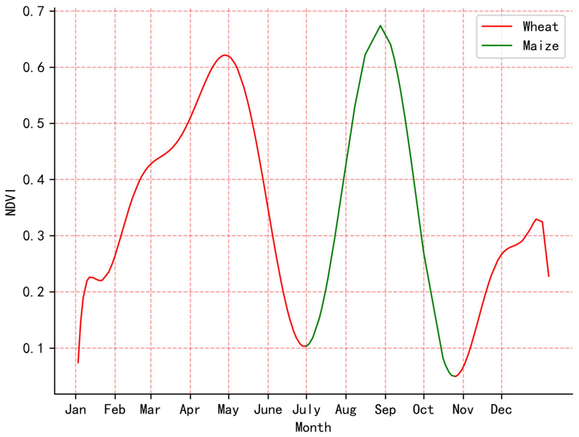
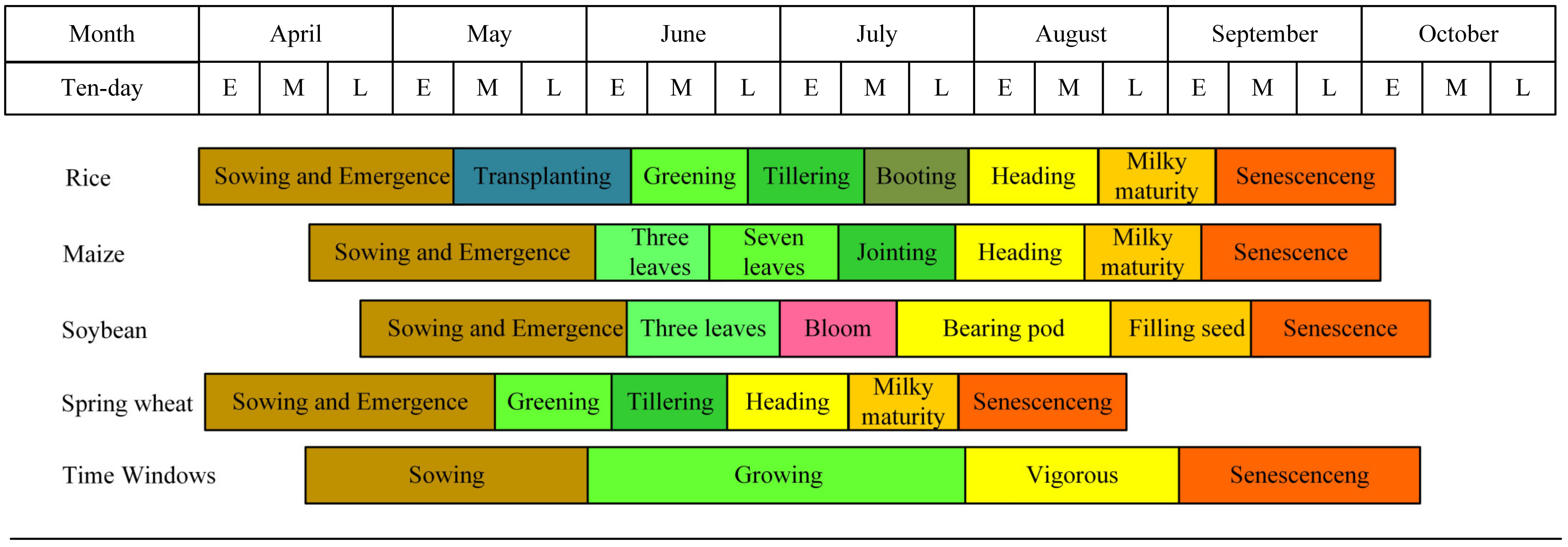
2.4. Phenological Features

Due to the influence of the temporal resolution and image quality of remote sensing images, obtaining images of every phenological stage of crops is difficult; therefore, the temporal image resolution requirement must be reduced, and the growth cycle of crops must be simplified to facilitate our temporal alignment using phenological stages. The complete NDVI time series dataset can better reflect the whole cultivation process of crops from sowing to growing, vigorous growth, maturation, and harvesting. This process is linked with the vegetation phenological period; therefore, NDVI time series curves can be used to extract key time windows that can both reduce the amount of classification data, accelerate the classification, and reduce the interference of invalid information on the classification.
In this paper, the NDVI time series curves of major crops in Northeast China and Shandong Province were established using Sentinel time series images and farm crop data. We downloaded the NDVI products of Sentinel 2 through the GEE platform and obtained the NDVI values of the corresponding locations based on the coordinates of the crops with tags. We downloaded NDVI datasets for 34-time nodes in Northeast China, and 46-time nodes in Shandong Province. Because factors such as clouds and aerosols can greatly affect NDVI data, it is necessary to smooth and denoise the NDVI time series set and reconstruct the NDVI time series. This paper uses a Savizky–Golay (S–G) filter for the smoothing and denoising process. The S–G filter is a moving-window weighted averaging algorithm derived by least-squares fitting of a given higher-order polynomial within a sliding window based on the following expression:
N D V I ( j , i ) = ( ρ N I R ρ R e d ) / ( ρ N I R + ρ R e d )
N D V I j = i = m i = m C i N D V I ( j , i ) N
where N D V I ( j , i ) denotes the original NDVI value of the i th pixel at time j , and N D V I j denotes the fitted NDVI value at time j after filtering; C i denotes the coefficient when the i th NDVI value is filtered; m is the half filter window width; and N is the filter length.
Northeast China and most of Inner Mongolia are located in the middle temperate zone, which is influenced by climate, and the crop rotation is annual, which shows only one wave peak on the NDVI time series curves, as shown in Figure 2. In addition, Shandong Province is in the warm temperate region of the northern hemisphere, and it presents significant continental monsoon climate characteristics, four distinct seasons, sufficient surface temperature, and a suitable climate, thus forming a biannual system with a winter wheat and summer maize rotation. Thus, the NDVI time series curve presents two wave peaks, as shown in Figure 3. Based on the analysis of the correspondence between the phenological calendar and the NDVI of the target crops, namely, maize, rice, and soybean, the crop growth cycle was redivided into four important time windows. They are sowing period, growing period, vigorous period, and harvesting period.
Based on the analysis of the correspondence between the phenological calendar and the NDVI of the target crops, namely, maize, rice, and soybean, the crop growth cycle was redivided into four important time windows. The first time window is the sowing period when the crop has no obvious features on the remote sensing images. In this window, soybean and maize have just been sown and the target cropland presents bare ground; however, due to the special sowing method of rice, the soaking/transplanting period of rice is observed in this window. The target cropland contrasts with other non-target vegetation, such as woodland and grassland, within this time window, and it is expressed in the NDVI curve as an inflection point from low to high. The second time window is the growing stage of rapid crop growth and development, and the crops in this period are characterized by rapid and unstable changes in remote sensing images within a short period, which is expressed in the NDVI curve as a fast-rising stage. The third time window is the vigorous period of crop growth (near the spike stage for maize and rice and near the pod stage for soybean), during which the NDVI reaches its peak, the leaf area reaches its maximum, photosynthesis is strong, the features of crops on remote sensing images are obvious, and the features of different crops differ greatly. This period is also an important period to distinguish wheat from target crops, because the phenological cycle of wheat is short, and wheat in this period has begun to be harvested. Thus, it is the most favorable period for distinguishing different crops. The fourth time window is the harvesting period from maturity to senescence. Due to the delay of harvesting, the state of cropland in this period is uneven because some crops on cropland have been harvested while other crops have not yet been harvested. This period is expressed in the NDVI curve as a rapid decline. Therefore, the sowing and vigorous periods are the two key time windows with the most different, prominent, and stable features. The centers of the time windows (Figure 4) are the inflection points for rapid increases and decreases of the NDVI. Images from these time windows within the study area were used as input to build our model.

3. Methodology

3.1. Off-Center Bayesian Deep Learning Network

To better incorporate the features of crop phenological changes and enhance the features of the vigorous period, a model structure based on the a priori knowledge of phenology is designed to thoroughly learn the phenological information in multi-temporal images. Unlike the traditional DL model, the posterior distribution of the weight parameters in BDL is represented as a probability distribution, which makes the trained model more tolerant to uncertainty and the model is more robust and generalizable, so we use BDL as a classifier. In terms of temporal feature extraction, a time-series feature fusion module is designed in this paper to capture the crop phenological relationships in temporal data by calculating the relationships between different temporal channels using the attention module. In addition, based on the analysis of the sowing period and the vigorous period phenological features, we design an off-center enhancement module to transfer shallow information to deeper layers in the vigorous period channel and deepen the feature extraction depth of the vigorous period. The model to improve separability between different crops by enhancing the vigorous period features is called off-center Bayesian deep learning (OCBDL). The structure of this model is shown in Figure 5.
In this model, the data from the sowing and vigorous periods are divided into two branches of the network, and each layer of the two branches is combined after convolution and goes through the time-series feature fusion module for temporal feature extraction. In addition, for the channel of the vigorous branch, we use the off-center enhancement module to enhance the extraction of the vigorous period features by transferring the shallow features to the deep features and enhancing the multiplexing of the vigorous features. Finally, the enhanced vigorous features are merged with the results of the temporal feature extraction, and the classification output is performed by the SoftMax function after convolution and full concatenation.

3.2. Off-Center Enhancement Module

Traditional convolutional or fully connected layers experience information loss during information transfer. Residual connection fuses shallow features with deeper features, which allows shallow features to be used in deeper layers, thereby increasing the reusability of shallow features and the learning efficiency of the network. As shown in Figure 6, we can use a nonlinear change function to describe the input and output of a network. For a network with input x l and output F ( x l ) , F ( x l ) usually includes operations such as convolution, normalization, and nonlinear activation. When we forcibly add an input to the output of the function, we can still use H l + 1 ( x l ) to describe the input–output relationship. This H l + 1 ( x l ) can be explicitly split into a linear superposition of F ( x l ) and x l using a corrected linear unit (RELU) to transform the fusion of shallow and deep features into a new feature representation:   x l + 1 = H l + 1 [ x l , F ( x l ) ] . This allows for the learning of deeper features while reducing the loss of underlying information.

3.3. Time-Series Feature Fusion Module

The time-series feature fusion module is based on a global attention mechanism that improves the performance of deep neural networks by increasing the interaction between different temporal feature channels. This module mainly includes global pooling, convolution, ReLu, and Sigmoid activation, as shown in Figure 7. In this module, we first merge the monophasic features of the subsidiary branches. Then, the merged features are pooled globally on average. The feature map is changed from a matrix of [h, w, c] to a vector of [1, 1, c], and then the information interaction between different timing channels is realized by one-dimensional convolution, and the size of the convolution kernel is determined by the adaptive function. Therefore, the layer with a larger number of channels can have more cross-channel interactions, and after convolution is activated by the ReLu function and the Sigmoid function, the model becomes more nonlinear and better fits the complex correlations between channels. The normalized weights of each channel are obtained, and the original input feature map is multiplied channel by channel to obtain the new feature layer after the information interaction to suppress useless information in a targeted manner, enhance the timing information, reduce the transmission and accumulation of redundant information in the network, and improve the classification accuracy.

3.4. Accuracy Evaluation Metrics

3.4.1. Pixel-Level Accuracy Evaluation

In this paper, the accuracy of the crop classification extraction results is evaluated by the overall accuracy (OA), F1 score, and intersection over union (IOU) ratio. OA refers to the ratio of the sum of the number of pixels in the correctly identified categories to the total number of pixels in the test image among all categories identified. Precision is the proportion of correct pixels in the prediction result, and Recall indicates the proportion of correct pixels in the ground truth. The Recall, OA, F1, and IOU formulas are as follows:
OA = TP + TN TP + TN + FP + FN
Precision = TP TP + FP
Recall = TP TP + FN
F 1 = 2 × Precision × Recall Precision + Recall
IOU = TP TP + FN + FP
where TP represents true positive, FP represents false positive, TN represents true negative, and FN represents false negative. TP + FP + TN + FN is the total number of samples.

3.4.2. Classification Uncertainty Evaluation

The uncertainty of the classification is not only affected by the dataset but also by the model. SoftMax can determine the probability that the predicted pixels belong to each category. Because the predictions are not given as explicit categories but as probability distributions, the uncertainty estimates can be derived directly from the predictions. Shannon entropy [40] considers the average amount of information contained in a predictive distribution. Results with low entropy values correspond to plausible predictions, while results with high entropy values correspond to significantly uncertain predictions. By sampling from the posterior distribution inferred by the BDL classifier, the uncertainty of the model is therefore considered as follows:
p ^ = 1 M i = 1 i p i
H ( p ^ ) = k p ^ k log 2 p ^ k
where p ^ represents the SoftMax output after M samples, k represents the number of categories, and p ^ k represents the probability that the pixel belongs to a certain category after sampling. H ( p ^ ) represents the degree of confusion of the information contained and is used here to measure the uncertainty of classification.

3.5. Implementation Details

The proposed model uses TensorFlow 1.14.0 as the deep learning framework, and the development language is Python. This paper uses Adam optimizer to optimize the network and update the parameters with the initial learning rate set to 0.001. To better train the model, the learning rate will be automatically adjusted as the training period increases to accelerate the convergence of the network combined with optimization. This paper uses a multiclass cross-entropy loss function as the loss function. There were a total of 80 epochs in the training process and the batch size was 1024. In addition, to ensure a fair comparison of different deep learning methods, all compared deep learning models have the same learning rate, epoch, and batch size settings. The RFC uses grid search and cross-validation for tuning, and the final RFC parameters are set as n_estimators of 60, max_features of 6, and max_depth of 13.

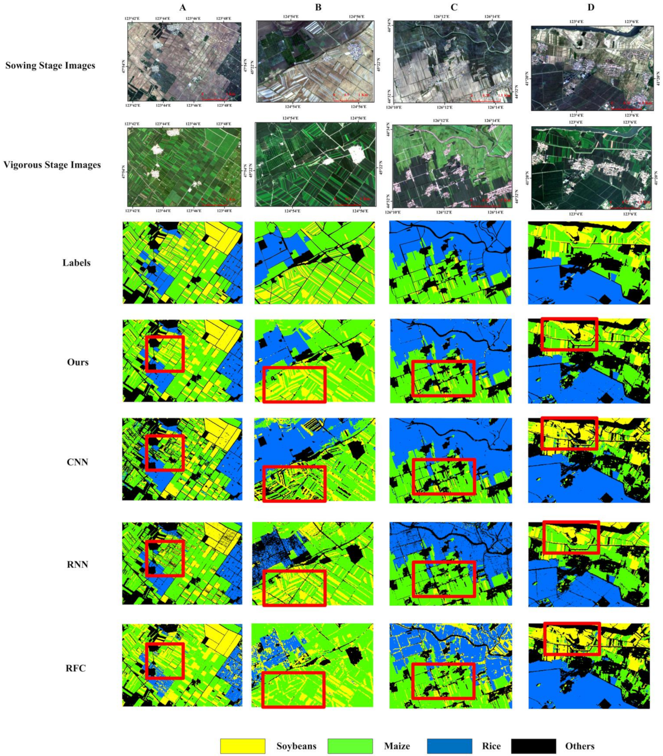
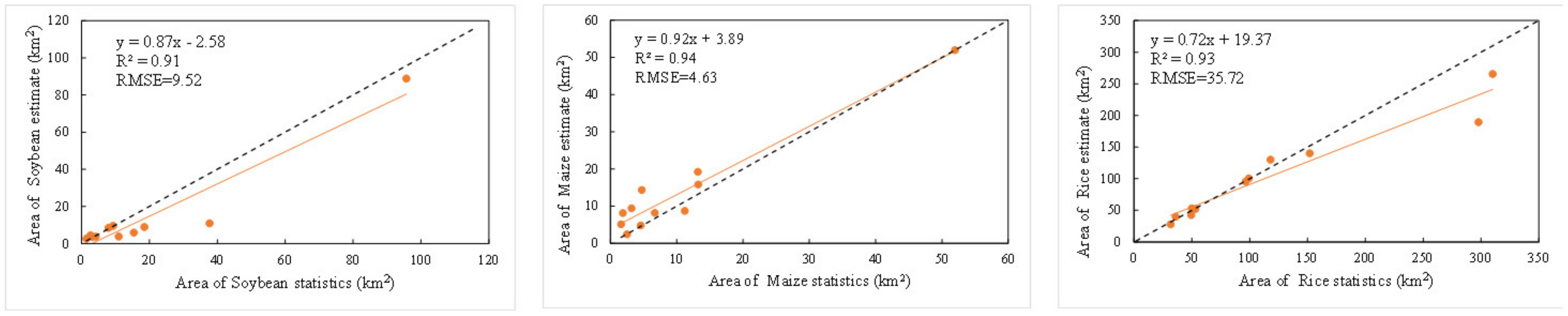
4. Results and Analysis

Based on the preparatory work and the constructed model, tests were conducted in four urban test areas that did not participate in the training. The image dates of the four test areas are 6 June 2019 and 30 August 2019 (A), 7 June 2021 and 6 August 2021 (B), 9 May 2019 and 1 September 2019 (C), and 12 June 2021 and 22 July 2021 (D), respectively. Details of the extraction results of the methods in this paper are shown in this section (Figure 8), and the classification results of this paper are compared with those of DL and machine learning models commonly used in crop classification. All models are trained from the same training data.
From Figure 8, it can be seen that among the four extraction methods, including the method of this paper, the overall extraction effect of the method of this paper is closest to the visual interpretation result, and the extraction results of CNN and RNN are slightly worse than the method of this paper. The red box in the figure shows the difference in details of the method in this paper compared to other methods. RNN is correct in the judgment of plot crop type, but there is a large amount of noise. The type of some plots of CNN is wrongly judged or not extracted. Still, the noise is less compared to RNN. This phenomenon is consistent with the advantages and disadvantages of RNN and CNN in crop extraction, as RNN focuses on temporal relationships. At the same time, CNN is more concerned with spatial contextual information. RFC has the worst extraction effect, and there are a large number of errors in the judgment of categories, and a large number of field ridges are incorrectly identified as soybeans and soybean plots are incorrectly identified as maize, which indicates that the feature extraction ability of RFC is worse than other networks.
From the perspective of qualitative analysis, the extraction results of OCBDL are more complete in all four urban tests, with almost no errors in the judgment of the class of the plots and less noise in the images, and they are very close to the real labels of the ground. To quantitatively verify the method’s performance in this paper, Table 1 lists the accuracy of the test results of different types of crops in each test area. The overall accuracy of the extraction results of the four test areas is 92.84%, 89.90%, 92.01%, and 88.15%. The average OA, F1, and IOU of the extraction results of the four test areas are 90.73%, 89.57%, and 81.48%; specifically for each category, the extraction results of soybean, maize, and rice reached 85.77%, 90.59%, and 92.34% on F1 and 75.70%, 82.91%, and 85.83% on IOU, respectively. The best extraction result among the three crops was rice, and the worst was soybean, which was due to the different degree of patch fragmentation. This is caused by the fact that, for the convenience of irrigation, rice is often planted in patches with a lower degree of fragmentation and therefore has a higher extraction accuracy. In contrast, soybean patches tend to be smaller in size and in slender strips, which results in soybean patches being more fragmented, especially in the C test area, where soybean patches are small. The extraction accuracy is the worst among the four test areas.
Table 2 list the average precision of the three crop extraction methods of this paper and CNN, RNN, and RFC in the four test areas. Regarding accuracy, RNN is the best performer among the other three crop classification models, except for this paper’s method. In the extraction results of RNN, the overall average precision of the four images OA, F1, and IOU are 85.99%, 84.56%, and 74.08%, which are lower than the methods in this paper by 4.74%, 5.01%, and 7.40%. Specifically for each category, the RNN model extracted F1 scores of 76.72%, 88.26%, and 88.69% for soybean, maize, and rice crop types, respectively, which were 9.05%, 2.33%, and 3.65% lower than the method of this paper, and IOUs of 63.44%, 79.02%, and 79.80%, respectively, which were 12.26%, 3.89%, and 6.03% lower than the method of this paper, which proves that the method in this paper outperforms other deep learning methods in crop classification extraction, no matter if they are type judgment or shape extraction. It is worth noting that although the overall classification accuracy of RNN is higher than that of CNN and RFC, the accuracy of soybean classification is the lowest among the four networks. Among the four classification models, the classification accuracy of soybean is the lowest among the three types of crops. However, the classification accuracy of soybean in this paper is still higher than that of other methods by more than 5%, indicating that this paper still performs better in classifying crop types with smaller patches and higher fragmentation compared with other methods.

5. Discussion

5.1. Uncertainty Analysis of Different Model Structures

In this subsection, to demonstrate the positive effects of the time-series feature fusion module and the off-center enhancement module on the network, we modified the networks as follows: the original BDL and the BDL networks containing the symmetrical enhancement module (SEBDL), the BDL networks containing the off-center enhancement module only at vigorous period channels (OCEBDL), the BDL networks containing only the time-series feature fusion module (T-BDL), and the off-center BDL network (OCBDL) proposed in this paper. The uncertainty distribution of the prediction results of the different models is shown in Figure 9, and the average classification accuracy evaluation of the other models in the four test areas is given in Table 3. Figure 9 shows that the classification results with higher uncertainty are mainly distributed on the ridge of the field. This uncertainty distribution can be explained by the ridge being located at the junctions between plots. Due to the resolution, the ridge contains many mixed pixels; therefore, the uncertainty is higher. Some pixels with higher uncertainty are distributed on other vegetation, caused by the similarity between vegetation types. The classification uncertainties of SEBDL, OCEBDL, and T-BDL are all decreased relative to that of the original BDL.
Table 3 shows that the OA, F1, and IOU of SEBDL, OCEBDL, and T-BDL are higher than that of the original BDL in all scenes; therefore, the residual linking module and attention module play an active role in crop classification. In addition, the OA, F1, and IOU of OCEBDL are improved by 1.18%, 1.33%, and 1.32%, respectively, relative to the symmetric SEBDL, which indicates that the asymmetric residual structure highlights the crop characteristics in the vigorous stage and enhances the differentiability among different crops. T-BDL has lower uncertainty in other vegetation relative to SEBDL, indicating that the attention mechanism effectively uses the temporal relationship to discriminate between diverse vegetation. OCBDL performs better in terms of the classification uncertainty of the ridge and other vegetation relative to the other networks, and the OA, F1, and IOU of OCBDL are improved by 5.46%, 6.08%, and 7.53%, respectively, relative to the original BDL. This result indicates that both the attention module and the residual linkage module are essential for our network and the model structure of OCBDL effectively reduces the classification uncertainty and improves the classification accuracy.

5.2. Validation of the Adaptability of the Method in Different Years

Based on the same simplified time window in 2019, we verified the generalizability of the method in different years in Suibin County, Heilongjiang Province, Northeast China, and the latest available set of statistics released by the Suibin County Bureau of Statistics as of May 2022 was the 2020 Statistical Yearbook. Therefore, we compared the county-level crop acreage statistics of Suibin County from 2018 to 2020 with the results obtained by the proposed method for the crop mapping area. The dates of the images used in the multi-year adaptation validation experiments in Suibin were 18 May 2018, 7 June 2019, 13 June 2020 (sowing period) and 16 August 2018, 31 August 2019, 22 August 2020 (vigorous period). As shown in Figure 10, Figure 11 and Figure 12, the 2018 Suibin County Statistical Yearbook contains statistics for only nine townships in Suibin County. The average coefficient of determination, R2, between the three crop mapping areas and the official statistical area was 0.897. The average RMSE was 9.55 km2, and the mapped area for maize was generally high compared to the official statistics, which was influenced by cloud shading in the images, which was occasionally incorrectly identified as maize. In 2019, the same year in which the NDVI curves were produced, the average coefficient of determination, R2, between the mapped area and the official statistics for the three crops was 0.926, and the average RMSE was 16.62 km2. The average coefficient of determination, R2, between the mapped area and the official statistics for the three crops was 0.933, and the average RMSE was 17.75 km2 in 2020. The excellent correlation between the soybean, maize, and rice crops estimated from Sentinel 2 satellite data and the official statistical area over 18–20 years indicates that the method in this paper has good adaptability in different years, which indicates that the same site can be continuously monitored for many years. In addition, there will be some differences between NDVI curves in different years and areas. Still, the crop phenology in Northeast China is similar, and using phenological stages aligned in different years in Northeast China can eliminate the need to establish NDVI curves each year. In Figure 13a–c, the distribution and changes in soybean maize and rice cultivation in Suibin County from 2018–2020 are shown.

5.3. Validation of the Adaptability of the Proposed Method in Areas with Different Cropping Structures

The method adaptation validation was first conducted in Heilongjiang province. According to the NDVI time series curve and phenological period, the date ranges of the images used in the adaptability verification experiment in Heilongjiang Province are 10 May 2020–10 June 2020 (sowing period) and 1 August 2020–1 September 2020 (vigorous period), respectively. Because of missing data in Daxinganling, Heihe, and Mudanjiang cities, we used the OCBDL model to draw crop maps for 11 cities in Heilongjiang province. The soybean, maize, and rice pixels estimated using the OCBDL were aggregated and compared with statistical data. As shown in Figure 14, the official statistics for soybean, maize, and rice for the 11 cities were 29,710, 48,663, and 38,060 km2, respectively, and the OCBDL model estimated 33,423, 49,386, and 42,446 km2 for soybean, maize, and rice for the 11 cities, respectively. The absolute errors for soybean, maize, and rice were 3713, 723, and 4386 km2, respectively, with relative errors of 0.115, 0.0148, and 0.125; R2 = 0.98 and RMSE = 3343.95. The influence of clouds, the shaded part of which was incorrectly identified as a crop, in addition to other crops not previously sampled by the model, lead to the over estimation of crop area by the OCBDL. The area distribution of soybean, maize, and rice planted in Heilongjiang Province in 2020 is shown in Figure 15.
Method adaptation validation was carried out in Shandong Province without any adjustment to the model, and summer maize was mapped in Shandong Province for the year 2020. We selected Sentinel 2 images corresponding to the sowing and vigorous period based on the NDVI curve of maize in Shandong province, and then input them into the model for prediction. According to the NDVI time series curve and phenological period, the date ranges of the images used in the adaptability verification experiment in Shandong Province are 10 June 2020–10 July 2020 (sowing period) and 10 August 2020–10 September 2020 (vigorous period). The input and output of the model were not adjusted, and for the extraction results of Shandong province we masked the results and only extracted maize as a class in the classification results; soybean and rice were classified as other classes. Summer maize pixels estimated using Sentinel 2A/B data were aggregated to the municipal level in Shandong Province and compared with municipal statistics. Compared with the other three methods (Figure 16a–d), the summer maize planted area method estimated using the OCBDL method best matched the municipal agricultural census data, with an R2 of 0.94 and RMSE of 370.26 km2. The summer maize planted area extracted by the RNN and CNN also showed a good correlation with the municipal agricultural census data, with R2 values of 0.91 and 0.86, respectively, while the RMSE values were 672.58 km2 and 750.96 km2, respectively. The estimated summer maize area in individual cities had significant errors relative to the statistical data. The summer maize area extracted using the RFC in Shandong Province was generally lower than the official statistical summer maize planted area, which indicated that the trained RFC is less adaptable in Shandong Province. Therefore, compared with other models, the method proposed in this paper is more adaptable in other regions, thus reflecting the advantage of OCBDL in terms of generalizability. The distribution of the maize cultivation area in Shandong Province in 2020 is shown in Figure 17.

6. Conclusions

This paper aimed to overcome the problems of uncertainty and generalizability observed in multi-time-series remote sensing crop classification, and it proposed the OCBDL multi-time-series remote sensing classification method based on phenology, which was used for large-area mapping of soybean, maize, and rice in different regions and years. This method uses the advantage of BDL, which can consider uncertainty, and combines this method with an attention mechanism and residual connection to reduce the uncertainty in the process of crop classification of remote sensing images. Sentinel 2A/B time series data were used to create crop NDVI time-series curves, and crop phenology information was combined to obtain key time windows, strengthen the differences among crops, and improve the accuracy of crop classification and the applicability of the model. In the precision verification experiments of the four test areas in Northeast China, the overall classification accuracy of the three crops reached 90.73% and the average F1 and average IOU were 89.57% and 81.48%, respectively. Thus, the proposed model outperformed the CNN, RNN, and RFC in crop classification judgment and plot integrity. In the uncertainty analysis experiment, the uncertainty of crop classification was mainly distributed in the mixed pixels of the plot boundary and some other vegetation pixels similar to the crops. The model structure based on the phenology design effectively reduced the uncertainty and improved the classification accuracy and completeness. The applicability of the model for crop classification in different years was verified in Suibin County, Heilongjiang Province, and the estimated planting areas of soybean, maize, and rice based on this method were strongly correlated with the statistical data. These findings show that the method proposed in this paper has good adaptability for crop mapping in different years. In the experiments with different climates and crop rotations from the training data, the estimated summer maize planted area in Shandong Province based on the method proposed in this paper showed good correlations and variance with the statistical data, with R2 = 0.94 and RMSE = 370.26 km2. The performance was better than that of the CNN, RNN, and RFC, indicating that the method of this paper still has good applicability under different climates and crop rotations. Although the method in this paper showed improved uncertainty and generalizability for multi-temporal remote sensing crop classification, many challenges remain in remote sensing estimations of crop acreage. For example, the plot size, clouds, and shadows still have influence on the crop acreage estimation. Therefore, further attention will be paid to these influencing factors in future research to find appropriate solutions.

Author Contributions

Conceptualization, Y.W. (Yongchuang Wu) and H.Y.; methodology, Y.W. (Yongchuang Wu); validation, Y.W. (Yanlan Wu); investigation, P.W. and B.W.; resources, P.W. and Y.W. (Yongchuang Wu); data curation, P.W. and B.W.; writing—original draft preparation, Y.W. (Yongchuang Wu); writing—review and editing, Y.W. (Yongchuang Wu) and H.Y.; funding acquisition, Y.W. (Yanlan Wu), H.Y. and B.W. All authors have read and agreed to the published version of the manuscript.

Funding

This research was funded by the National Natural Science Foundation of China (grant Nos. 42101381, 41901282, and 41971311) and the funders are Hui Yang, Yanlan Wu and Biao Wang, the National Natural Science Foundation of Anhui (grant No. 2008085QD188) and the funder is Yanlan Wu, the Science and Technology Major Project of Anhui Province (grant No. 201903a07020014) and the funder is Yanlan Wu, and the Anhui Provincial Key R&D International Cooperation Program (grant No. 202104b11020022) and the funder is Yanlan Wu.

Institutional Review Board Statement

Not applicable.

Informed Consent Statement

Not applicable.

Data Availability Statement

The data presented in this study are available on request from the corresponding author. The data are not publicly available due to the permissions issues.

Conflicts of Interest

The authors declare no conflict of interest.

References

  1. Foley, J.A.; Ramankutty, N.; Brauman, K.A.; Cassidy, E.S.; Gerber, J.S.; Johnston, M.; Mueller, N.D.; O’Connell, C.; Ray, D.K.; West, P.C.; et al. Solutions for a Cultivated Planet. Nature 2011, 478, 337–342. [Google Scholar] [CrossRef] [Green Version]
  2. Godfray, H.C.J.; Beddington, J.R.; Crute, I.R.; Haddad, L.; Lawrence, D.; Muir, J.F.; Pretty, J.; Robinson, S.; Thomas, S.M.; Toulmin, C. Food Security: The Challenge of Feeding 9 Billion People. Science (80-) 2010, 327, 812–818. [Google Scholar] [CrossRef] [Green Version]
  3. Biradar, C.M.; Thenkabail, P.S.; Noojipady, P.; Li, Y.; Dheeravath, V.; Turral, H.; Velpuri, M.; Gumma, M.K.; Gangalakunta, O.R.P.; Cai, X.L.; et al. A Global Map of Rainfed Cropland Areas (GMRCA) at the End of Last Millennium Using Remote Sensing. Int. J. Appl. Earth Obs. Geoinf. 2009, 11, 114–129. [Google Scholar] [CrossRef]
  4. Teluguntla, P.; Thenkabail, P.; Oliphant, A.; Xiong, J.; Gumma, M.K.; Congalton, R.G.; Yadav, K.; Huete, A. A 30-m Landsat-Derived Cropland Extent Product of Australia and China Using Random Forest Machine Learning Algorithm on Google Earth Engine Cloud Computing Platform. ISPRS J. Photogramm. Remote Sens. 2018, 144, 325–340. [Google Scholar] [CrossRef]
  5. Yuan, Q.; Shen, H.; Li, T.; Li, Z.; Li, S.; Jiang, Y.; Xu, H.; Tan, W.; Yang, Q.; Wang, J.; et al. Deep Learning in Environmental Remote Sensing: Achievements and Challenges. Remote Sens. Environ. 2020, 241, 111716. [Google Scholar] [CrossRef]
  6. Foerster, S.; Kaden, K.; Foerster, M.; Itzerott, S. Crop Type Mapping Using Spectral-Temporal Profiles and Phenological Information. Comput. Electron. Agric. 2012, 89, 30–40. [Google Scholar] [CrossRef] [Green Version]
  7. Mingwei, Z.; Qingbo, Z.; Zhongxin, C.; Jia, L.; Yong, Z.; Chongfa, C. Crop Discrimination in Northern China with Double Cropping Systems Using Fourier Analysis of Time-Series MODIS Data. Int. J. Appl. Earth Obs. Geoinf. 2008, 10, 476–485. [Google Scholar] [CrossRef]
  8. Conrad, C.; Dech, S.; Dubovyk, O.; Fritsch, S.; Klein, D.; Löw, F.; Schorcht, G.; Zeidler, J. Derivation of Temporal Windows for Accurate Crop Discrimination in Heterogeneous Croplands of Uzbekistan Using Multitemporal RapidEye Images. Comput. Electron. Agric. 2014, 103, 63–74. [Google Scholar] [CrossRef]
  9. Valero, S.; Morin, D.; Inglada, J.; Sepulcre, G.; Arias, M.; Hagolle, O.; Dedieu, G.; Bontemps, S.; Defourny, P.; Koetz, B. Production of a Dynamic Cropland Mask by Processing Remote Sensing Image Series at High Temporal and Spatial Resolutions. Remote Sens. 2016, 8, 55. [Google Scholar] [CrossRef] [Green Version]
  10. Devadas, R.; Denham, R.J.; Pringle, M. Support Vector Machine Classification of Object-Based Data for Crop Mapping, Using Multi-Temporal Landsat Imagery. Int. Arch. Photogramm. Remote Sens. Spat. Inf. Sci. 2012, XXXIX-B7, 185–190. [Google Scholar] [CrossRef]
  11. Kumar, P.; Gupta, D.K.; Mishra, V.N.; Prasad, R. Comparison of Support Vector Machine, Artificial Neural Network, and Spectral Angle Mapper Algorithms for Crop Classification Using LISS IV Data. Int. J. Remote Sens. 2015, 36, 1604–1617. [Google Scholar] [CrossRef]
  12. Shao, Y.; Lunetta, R.S. Comparison of Support Vector Machine, Neural Network, and CART Algorithms for the Land-Cover Classification Using Limited Training Data Points. ISPRS J. Photogramm. Remote Sens. 2012, 70, 78–87. [Google Scholar] [CrossRef]
  13. Song, X.P.; Potapov, P.V.; Krylov, A.; King, L.A.; Di Bella, C.M.; Hudson, A.; Khan, A.; Adusei, B.; Stehman, S.V.; Hansen, M.C. National-Scale Soybean Mapping and Area Estimation in the United States Using Medium Resolution Satellite Imagery and Field Survey. Remote Sens. Environ. 2017, 190, 383–395. [Google Scholar] [CrossRef]
  14. Xu, J.; Zhu, Y.; Zhong, R.; Lin, Z.; Xu, J.; Jiang, H.; Huang, J.; Li, H.; Lin, T. DeepCropMapping: A Multi-Temporal Deep Learning Approach with Improved Spatial Generalizability for Dynamic Corn and Soybean Mapping. Remote Sens. Environ. 2020, 247, 111946. [Google Scholar] [CrossRef]
  15. Zhong, L.; Hawkins, T.; Biging, G.; Gong, P. A Phenology-Based Approach to Map Crop Types in the San Joaquin Valley, California. Int. J. Remote Sens. 2011, 32, 7777–7804. [Google Scholar] [CrossRef]
  16. Rubwurm, M.; Korner, M. Temporal Vegetation Modelling Using Long Short-Term Memory Networks for Crop Identification from Medium-Resolution Multi-Spectral Satellite Images. In Proceedings of the IEEE Conference on Computer Vision and Pattern Recognition (CVPR) Workshops, Honolulu, HI, USA, 21–26 July 2017; pp. 1496–1504. [Google Scholar] [CrossRef]
  17. Ndikumana, E.; Minh, D.H.T.; Baghdadi, N.; Courault, D.; Hossard, L. Deep Recurrent Neural Network for Agricultural Classification Using Multitemporal SAR Sentinel-1 for Camargue, France. Remote Sens. 2018, 10, 1217. [Google Scholar] [CrossRef] [Green Version]
  18. Huang, B.; Zhao, B.; Song, Y. Urban Land-Use Mapping Using a Deep Convolutional Neural Network with High Spatial Resolution Multispectral Remote Sensing Imagery. Remote Sens. Environ. 2018, 214, 73–86. [Google Scholar] [CrossRef]
  19. Marcos, D.; Volpi, M.; Kellenberger, B.; Tuia, D. Land Cover Mapping at Very High Resolution with Rotation Equivariant CNNs: Towards Small yet Accurate Models. ISPRS J. Photogramm. Remote Sens. 2018, 145, 96–107. [Google Scholar] [CrossRef] [Green Version]
  20. Lu, Y.; Li, H.; Zhang, S. Multi-Temporal Remote Sensing Based Crop Classification Using a Hybrid 3D-2D CNN Model. Nongye Gongcheng Xuebao/Trans. Chin. Soc. Agric. Eng. 2021, 37, 13. [Google Scholar] [CrossRef]
  21. Li, Z.; Chen, G.; Zhang, T. A CNN-Transformer Hybrid Approach for Crop Classification Using Multitemporal Multisensor Images. IEEE J. Sel. Top. Appl. Earth Obs. Remote Sens. 2020, 13, 847–858. [Google Scholar] [CrossRef]
  22. Garnot, V.S.F.; Landrieu, L.; Giordano, S.; Chehata, N. Time-Space Tradeoff in Deep Learning Models for Crop Classification on Satellite Multi-Spectral Image Time Series. In Proceedings of the IGARSS 2019–2019 IEEE International Geoscience and Remote Sensing Symposium, Yokohama, Japan, 28 July–2 August 2019; pp. 6247–6250. [Google Scholar] [CrossRef] [Green Version]
  23. Rußwurm, M.; Körner, M. Self-Attention for Raw Optical Satellite Time Series Classification. ISPRS J. Photogramm. Remote Sens. 2020, 169, 421–435. [Google Scholar] [CrossRef]
  24. Castro, J.B.; Feitosa, R.Q.; Happ, P.N. An Hybrid Recurrent Convolutional Neural Network for Crop Type Recognition Based on Multitemporal SAR Image Sequences. In Proceedings of the IGARSS 2018–2018 IEEE International Geoscience and Remote Sensing Symposium, Valencia, Spain, 22–27 July 2018; pp. 3824–3827. [Google Scholar] [CrossRef]
  25. Chamorro Martinez, J.A.; Cué La Rosa, L.E.; Feitosa, R.Q.; Sanches, I.D.A.; Happ, P.N. Fully Convolutional Recurrent Networks for Multidate Crop Recognition from Multitemporal Image Sequences. ISPRS J. Photogramm. Remote Sens. 2021, 171, 188–201. [Google Scholar] [CrossRef]
  26. Chen, Y.; Song, X.; Wang, S.; Huang, J.; Mansaray, L.R. Impacts of Spatial Heterogeneity on Crop Area Mapping in Canada Using MODIS Data. ISPRS J. Photogramm. Remote Sens. 2016, 119, 451–461. [Google Scholar] [CrossRef]
  27. Löw, F.; Knöfel, P.; Conrad, C. Analysis of Uncertainty in Multi-Temporal Object-Based Classification. ISPRS J. Photogramm. Remote Sens. 2015, 105, 91–106. [Google Scholar] [CrossRef]
  28. Löw, F.; Michel, U.; Dech, S.; Conrad, C. Impact of Feature Selection on the Accuracy and Spatial Uncertainty of Per-Field Crop Classification Using Support Vector Machines. ISPRS J. Photogramm. Remote Sens. 2013, 85, 102–119. [Google Scholar] [CrossRef]
  29. Biggs, T.W.; Thenkabail, P.S.; Gumma, M.K.; Scott, C.A.; Parthasaradhi, G.R.; Turral, H.N. Irrigated Area Mapping in Heterogeneous Landscapes with MODIS Time Series, Ground Truth and Census Data, Krishna Basin, India. Int. J. Remote Sens. 2006, 27, 4245–4266. [Google Scholar] [CrossRef]
  30. Turker, M.; Arikan, M. Sequential Masking Classification of Multi-Temporal Landsat7 ETM+ Images for Field-Based Crop Mapping in Karacabey, Turkey. Int. J. Remote Sens. 2005, 26, 3813–3830. [Google Scholar] [CrossRef]
  31. Zhong, L.; Gong, P.; Biging, G.S. Efficient Corn and Soybean Mapping with Temporal Extendability: A Multi-Year Experiment Using Landsat Imagery. Remote Sens. Environ. 2014, 140, 1–13. [Google Scholar] [CrossRef]
  32. Wang, H.; Yeung, D.Y. A Survey on Bayesian Deep Learning. ACM Comput. Surv. 2020, 53, 1–37. [Google Scholar] [CrossRef]
  33. Kendall, A.; Gal, Y. What Uncertainties Do We Need in Bayesian Deep Learning for Computer Vision? In Proceedings of the Advances in Neural Information Processing Systems 30 (NIPS 2017), Long Beach, CA, USA, 4–9 December 2017; pp. 5575–5585. [Google Scholar]
  34. Mena, J.; Catalunya, C.T.D.; Matemàtiques, D.D. A Survey on Uncertainty Estimation in Deep Learning. ACM Comput. Surv. (CSUR) 2021, 54, 1–35. [Google Scholar] [CrossRef]
  35. Hern, D.; Tom, F.; Adams, R.P. Predictive Entropy Search for Multi-Objective Bayesian Optimization. arXiv 2014, arXiv:1511.05467v3. [Google Scholar]
  36. Vaswani, A.; Shazeer, N.; Parmar, N.; Uszkoreit, J.; Jones, L.; Gomez, A.N.; Kaiser, Ł.; Polosukhin, I. Attention Is All You Need. In Proceedings of the Advances in Neural Information Processing Systems, Long Beach, CA, USA, 4–9 December 2017. [Google Scholar]
  37. Xu, J.; Yang, J.; Xiong, X.; Li, H.; Huang, J.; Ting, K.C.; Ying, Y.; Lin, T. Towards Interpreting Multi-Temporal Deep Learning Models in Crop Mapping. Remote Sens. Environ. 2021, 264, 112599. [Google Scholar] [CrossRef]
  38. Friedl, M.A.; Brodley, C.E.; Strahler, A.H. Maximizing Land Cover Classification Accuracies Produced by Decision Trees at Continental to Global Scales. IEEE Trans. Geosci. Remote Sens. 1999, 37, 969–977. [Google Scholar] [CrossRef]
  39. Geerken, R.A. An Algorithm to Classify and Monitor Seasonal Variations in Vegetation Phenologies and Their Inter-Annual Change. ISPRS J. Photogramm. Remote Sens. 2009, 64, 422–431. [Google Scholar] [CrossRef]
  40. Shannon, C.E. A Mathematical Theory of Communication. Bell Syst. Tech. J. 1948, 27, 379–423. [Google Scholar] [CrossRef]
Figure 1. (AD) Geographical location of the study area and distribution of training data and validation area.
Remotesensing 15 00674 g001
Figure 2. NDVI time series curves of major important crops in Northeast China.
Remotesensing 15 00674 g002
Figure 3. NDVI time series curve of wheat and maize in Shandong Province in 2020.
Remotesensing 15 00674 g003
Figure 4. Phenological calendar of major crops and simplified phenological time window.
Remotesensing 15 00674 g004
Figure 5. The structure of OCBDL.
Remotesensing 15 00674 g005
Figure 6. Off-center enhancement module.
Remotesensing 15 00674 g006
Figure 7. Time-series feature fusion module.
Remotesensing 15 00674 g007
Figure 8. (AD) Input images of four test areas and test results of different models. The red wireframe shows the difference in detail.
Remotesensing 15 00674 g008
Figure 9. (AD) Uncertainty distribution of the classification results of different model structures in the four test areas. The black wireframe shows the difference in detail.
Remotesensing 15 00674 g009
Figure 10. Correlation of the model−estimated main crop area with the statistical area in 2018.
Remotesensing 15 00674 g010
Figure 11. Correlation of the model−estimated main crop area with the statistical area in 2019.
Remotesensing 15 00674 g011
Figure 12. Correlation of the model−estimated main crop area with the statistical area in 2020.
Remotesensing 15 00674 g012
Figure 13. (a) Distribution of the main crop cultivation area in Suibin County in 2018. (b) Distribution of the main crop cultivation area in Suibin County in 2019. (c) Distribution of the main crop cultivation area in Suibin County in 2020.
Remotesensing 15 00674 g013aRemotesensing 15 00674 g013b
Figure 14. Crop areas recorded in the Statistical Yearbook for 11 cities in Heilongjiang Province in 2020 and the crop areas extracted by OCBDL.
Remotesensing 15 00674 g014
Figure 15. Sowing and vigorous images and OCBDL−estimated crop distribution in 11 cities in Heilongjiang Province.
Remotesensing 15 00674 g015
Figure 16. (ad). Estimated area of different models vs. the statistical area. The dotted line in the figure represents the 1:1 line, and the orange line is the estimated data fit line.
Remotesensing 15 00674 g016
Figure 17. OCBDL mapping of the distribution of the maize cultivated area in Shandong Province in 2020.
Remotesensing 15 00674 g017
Table 1. The classification accuracy of crop classification, based on the OCBDL. (%).
ImagesSoybeansMaizeRiceAverage
F1
Average
IOU
OA
F1IOUF1IOUF1IOU
A93.3587.5393.6688.0794.0288.7293.6888.1192.84
B86.7476.5991.3484.0691.8384.9089.9781.8589.90
C74.6759.5891.0483.5693.8788.4586.5377.2092.01
D88.3379.1086.3375.9589.6581.2488.1078.7688.15
Average85.7775.7090.5982.9192.3485.8389.5781.4890.73
Table 2. The classification accuracy of crop classification using the different methods. (%).
ModelSoybeansMaizeRiceAverage F1Average IOUOA
F1IOUF1IOUF1IOU
OCBDL85.7775.7090.5982.9192.3485.8389.5781.4890.73
CNN79.5866.3682.1170.8186.4476.4882.7171.2184.75
RNN76.7263.4488.2679.0288.6979.8084.5674.0885.99
RFC79.4835.8173.1558.7272.1058.2764.9150.9174.01
Table 3. Evaluation metric results for the ablation experiments. (%).
ModelSoybeansMaizeRiceAverage F1Average IOUOA
F1IOUF1IOUF1IOU
OCBDL85.7775.7090.5982.9192.3485.8389.5781.4890.73
T-BDL80.1167.9287.3378.2989.7782.2085.7476.1488.23
OCEBDL79.6068.4386.7578.4688.6581.6185.0076.1788.06
SEBDL79.1768.0585.1576.6287.1679.8683.8274.8486.74
BDL77.2865.1585.3076.3187.8980.4083.4973.9585.27
Disclaimer/Publisher’s Note: The statements, opinions and data contained in all publications are solely those of the individual author(s) and contributor(s) and not of MDPI and/or the editor(s). MDPI and/or the editor(s) disclaim responsibility for any injury to people or property resulting from any ideas, methods, instructions or products referred to in the content.

