Article

Study on Regional Eco-Environmental Quality Evaluation Considering Land Surface and Season Differences: A Case Study of Zhaotong City

1
School of Geography Science and Geomatics Engineering, Suzhou University of Science and Technology, Suzhou 215009, China
2
College of Resources and Environment, Xingtai University, Xingtai 054001, China
3
Xingtai Key Laboratory of Geo-Information and Remote Sensing Technology Application, Xingtai 054001, China
4
China Satellite Communications Co., Ltd., Beijing 100190, China
5
Northwest Institute of Eco-Environment and Resources, Chinese Academy of Sciences, Lanzhou 730000, China
6
Department of Geography and Environmental Studies, Wollo University, Dessie P.O. Box 1145, Ethiopia
7
Aerospace Information Research Institute, Chinese Academy of Sciences, Beijing 100094, China
8
School of Geomatics Science and Technology, Nanjing Tech University, Nanjing 211816, China
*
Author to whom correspondence should be addressed.
Remote Sens. 2023, 15(3), 657; https://doi.org/10.3390/rs15030657
Submission received: 20 November 2022 / Revised: 14 January 2023 / Accepted: 21 January 2023 / Published: 22 January 2023

Abstract

:
Timely and quantitatively evaluating regional eco-environmental quality (EEQ) is of great significance for realizing regional sustainable development goals. Especially for cloudy areas, it was a great challenge to construct a regional EEQ dataset with high quality and high resolution. However, existing studies failed to consider the influence of land surface and season elements in evaluating regional EEQ. Therefore, this study aimed to promote an accurate EEQ-evaluating framework for cloudy areas. Zhaotong city, a typical karst and cloudy region, was chosen as the study area. First, we integrated multi-source spatiotemporal datasets and constructed a novel eco-environmental comprehensive evaluation index (ECEI) to assess its EEQ from 2000 to 2020. Next, standard deviation ellipse (SDE) and trend analysis methods were applied to investigate regional EEQ’s change trends. Finally, ecological index (EI) values for different years were calculated to validate the effectivity of the ECEI. The main findings were as follows: (1) The EEQ of Zhaotong showed an upward-fluctuating trend (0.0058 a−1), with average ECEI values of 0.729, 0.693, 0.722, 0.749, and 0.730. (2) The spatial distribution pattern of the EEQ showed high values in the north and low values in the south, with Zhaoyang district having the lowest ECEI value. (3) From 2000 to 2020, the standard deviation of the major axis of the ellipse moved northeast of Zhaotong city with θ of SDE changing from 57.06° to 62.90°, thus, indicating the improvement of northeastern regions’ EEQ. (4) The coefficients of the determinant (R2) between the EI and ECEI were 0.84, which was higher than that of EI–RSEI (R2 = 0.56). This indicated that our promoted framework and the ECEI could acquire more accurate EEQ results and provide suggestions for relevant policymakers.

1. Introduction

Since the Industrial Revolution, the urbanization of the whole world has increased dramatically [1]. Based on the United Nations report issued in 2014, the world’s urbanization rate is expected to reach 66% in 2050 [2]. Especially in China, since the implementation of the reform and opening-up policy, the urbanization rate has increased from 17.92% in 1978 to 64.72% in 2021, with an average annual growth rate of 103.03% [3]. However, with the rapid development of urbanization, a series of problems have arisen, for example, degradation of land quality and soil erosion [4,5], decrease in biodiversity and vegetation coverage [6,7], intensification of heat island effect [8,9], a decline of air quality [10,11], and deterioration of eco-environment [12]. In response to these problems, the Chinese government carried out a regional, coordinated development strategy in 2017 [13], aiming to decrease the gap between different regions and promote coordinated development between the eco-environment and urbanization. Specifically, it is necessary to improve these eco-environment issues from the perspective of green infrastructure and urban sprawl. Urban green infrastructure is defined as “a strategically planned network of natural and semi-natural areas with other environmental features designed and managed to deliver a wide range of ecosystems services” [14]. Marando et al. used European functional urban areas to study the influence of the implementation of urban green infrastructure in mitigating the urban heat island effect, and they found that a tree cover of at least 16% was required to achieve a l ℃ drop in urban temperatures [14]. Donati et al. found that the planning of blue-green infrastructure could promote the permeability and availability of “stepping stone” habitats in densely populated landscapes, indicating that the blue and green infrastructure construction was of great help in maintaining regional habitat connectivity [15]. When Chanchipricha and Fischer evaluated the impact of developing urban green infrastructure, they suggested that environmental impact assessment should consider green infrastructure [16]. Barbosa et al. concluded that there was a disconnect and disarticulation between public spaces and green areas [17]. In general, green infrastructure construction could provide some influence on promoting an urban eco-environment, including the mitigation of the urban heat island effect and the maintenance of regional habitat connectivity.
As for urban sprawl, its influence on the regional EEQ is complicated. Ewing and Hamidi found that sprawling areas had higher ozone levels than compact areas [18]. Polidoro et al. found that urban sprawl could lead to the consequences of territorial ordering and the egalitarian spatial distribution of essential services [19]. Tian et al. concluded that planning was strongly correlated with urban sprawl, which was kind of a “planned sprawl” [20]. Huang et al. took eight landscape metrics to analyze the spatiotemporal changes in landscape patterns, indicating that a guiding plan was required to integrate planning in both urban and non-urban planned districts [21]. Barbosa and Pradilla concluded that the degree of vulnerability encountered by the social urban spatial structure was higher in expansion areas than in central areas [22]. Generally, urban sprawl, to some extent, could influence the regional EEQ. Thus, it is important to integrate planning to guide the direction of urban sprawl. Therefore, to realize this goal, it is urgent to evaluate the regional eco-environmental quality (EEQ) timely and quantitatively.
The definition of an eco-environment is the total quantity and quality of water resources, land resources, biological resources, and climate resources that affect human survival and development [23]. Evaluation of the EEQ normally consisted of two parts, which were the construction of a scientific index system and an accurate assessment of the regional EEQ [24]. To date, many scholars have promoted numerous novel indexes to evaluate the regional EEQ. For example, Fu developed a comprehensive index system to evaluate the regional EEQ at the provincial scale; this index system included water and soil loss, land salinization, agricultural natural disasters, land resources, water resources, forest resources, air pollution, water pollution, solid waste pollution, population, economic development, and township enterprises. However, all used datasets were acquired from national statistical yearbooks [25]. He et al. combined fine particulate matter (PM2.5) concentration, land surface temperature (LST), and vegetation cover (VC) to develop a comprehensive evaluation index (CEI), and he found that the increase of PM2.5 concentration had a great influence on the regional EEQ. Specifically, degraded regions were mainly distributed in expanded urban areas with an increased PM2.5 concentration [26]. Wei et al. integrated the normalized difference vegetation index (NDVI), wetness index, albedo, index-based built-up index, salinization index, and LST to construct an environmental quality index. In their study, weights of multiple indicators were objectively determined by the eigenvalues of all principal components. In addition, they found that the EEQ of urban regions displayed a damaging trend [27]. Chang et al. used the average annual precipitation, net primary productivity (NPP), elevation, biological abundance index (BAI), highway net density, and other nine indexes to establish an ecological environmental index (EEI). In their study, four climate aspects, such as soil–terrain, biological resources, and human factors were used to evaluate the regional EEQ. They also found that human factors had a negative influence on the regional EEQ [28]. Sun et al. calculated the NDVI, habitat quality index, normalized difference moisture index (NDMI), and normalized difference soil index (NDSI) to promote an eco-environmental quality index (EQI). Among them, threshold values were set to divide each index into different types. In addition, they also came to the conclusion that residential regions had poor EEQ [29]. Wei et al. selected twenty-three indices from hydro-meteorological, socioeconomic, soil, biological, and topographical aspects to construct an environmental vulnerability distance index (EVDI). Similar to the aforementioned studies, land use changes and human activities indirectly influenced the results of environmental vulnerability [30]. Chai and Lha chose sixty-six indexes from aspects of human activity and the natural environment to evaluate different regions’ EEQ; however, it took a long time to collect these data [31]. Ariken et al. built an index system from level, pollution, and protection aspects to evaluate the regional EEQ. Numerous indexes were calculated or acquired by statistical yearbooks [32]. To sum up, the data sources used in existing studies could be divided into two types: statistical data and non-statistical data [33]. Statistical data has the advantage of high authority. However, its data is mainly at the administrative scale, which fails to acquire the index value of any location [34]. Hence, in the previous studies, the regional EEQ was evaluated qualitatively. At the same time, it failed to detect EEQ changes at the grid level. Among non-statistical data, remote sensing data are one of the most widely used due to the advantages of wide space coverage and strong time continuity [35]. EEQ’s evaluation based on remote sensing datasets provided a useful way to detect EEQ changes at multi-dimensions, such as degradation of the EEQ caused by urban sprawl and human negative activities. To date, numerous indexes have been proposed to evaluate the regional EEQ, such as NDVI for vegetation detection [36] and LST for urban heat islands [37]. However, a single index could only reflect one aspect of the regional eco-environment, which fails to evaluate the regional comprehensive EEQ [38]. Compared with a single index, the aggregated index showed great potential. Especially, the remote sensing ecological index (RSEI) integrated four aspects, such as greenness, wetness, dryness, and heat, to evaluate the regional EEQ [39]. Since its promotion in 2013, numerous studies have applied this index to evaluate the regional EEQ at various scales [40,41,42,43,44]. However, the RSEI had some limitations in practical applications, including the influence of season, the effect of water bodies, lack of consideration for the land surface difference, and lack of application in cloudy areas. In response to the first three shortcomings, Xu et al. combined the land use data to develop the RSEI-2 to assess China’s EEQ [45]. Zhang et al. assessed Tianjin’s EEQ by combining the RSEI and season [46]. Xu and Deng suggested that it was not suitable to name these indexes as RSEI or use RSEI-related names when considering non-ecological factors [47]. Moreover, existing studies failed to consider both land surface and season differences. As for the fourth shortcoming, numerous studies adopted Google Earth Engine (GEE) platform to evaluate the regional EEQ by filtering satisfied images [48,49,50].
Generally, EEQ evaluation achieved fruitful results; however, cloudy regions’ EEQ evaluation considering both land surface and season differences has not been reported. This study aimed to promote an accurate EEQ-evaluating framework for cloudy areas and provide constant regional EEQ datasets with high quality and high resolution. Zhaotong city, a typical cloudy and karst area in China, was chosen as a study area to evaluate its EEQ from 2000 to 2020 as, during this period, the economic and social level of Zhaotong increased significantly. In addition, several high-accuracy datasets, such as land use datasets, have been available since 2000. First, Zhaotong’s cloudy-free Landsat series images from different seasons were filtered based on the GEE platform. Then, the results from the abundance index (AI) and four other indexes obtained in different seasons were integrated to establish a novel eco-environmental comprehensive evaluation index (ECEI). Finally, the ECEI results of were analyzed based on standard deviation ellipse (SDE) and trend analysis methods and compared with the ecological index (EI) developed by the Ministry of Ecology and Environment. This study is organized as follows: the Section 2 presents the general situations of the study area and adopted methodologies, which include calculation methods of the ECEI, EI, SDE, and trend analysis; the Section 3 describes the spatiotemporal distribution of the ECEI at different scales and the spatiotemporal change trend of the ECEI based on SDE and trend analysis methods; the Section 4 analyzes the spatial principal component analysis (SPCA) results, compares the ECEI results with the EI, and displays the implications and limitations of this study; the Section 5 shows this study’s main results and findings.

2. Materials and Methods

2.1. Study Area

Zhaotong is located in the northeastern part of Yunnan Province in China and the hinterland of the Wumeng Mountains on the border of Yunnan, Guizhou, and Sichuan provinces (Figure 1). It is also a typical karst region [51]. Zhaotong has a highland monsoon climate, with 96% of its territory covered by mountainous areas. It is rich in water resources, with an average annual precipitation of about 1120 mm and an uneven spatial and temporal distribution of rainfall, with the flood season concentrated in May–October. In 2020, the population and gross domestic product of Zhaotong were 5.09 million people and 128.87 billion yuan [52].

2.2. Data Sources and Processing
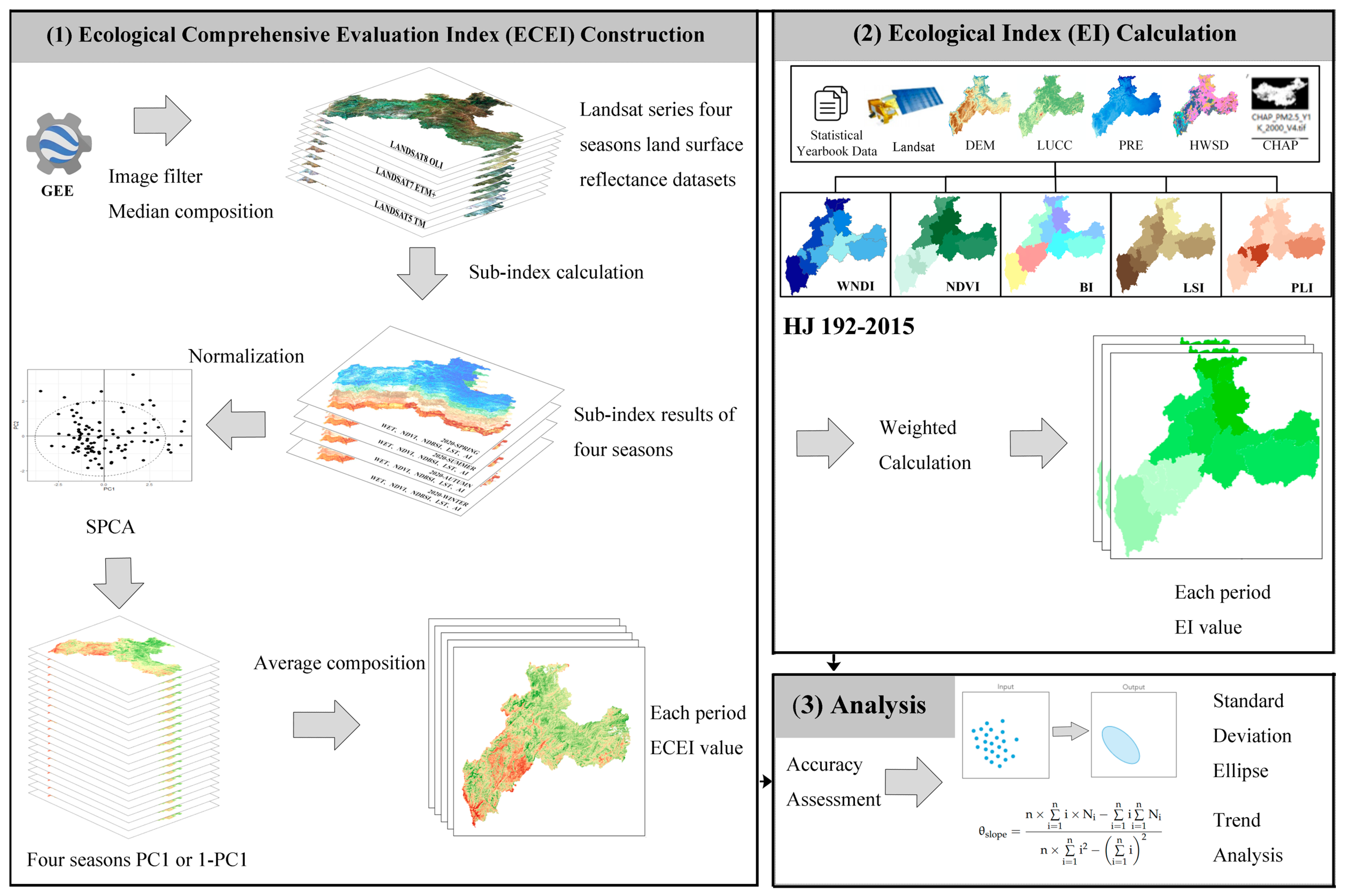
The study adopted multiple remote sensing datasets and administrative boundary data to evaluate Zhaotong’s EEQ. A brief introduction of each dataset is shown in Table 1.
Based on Table 1, Landsat 5, 7, and 8 images, land surface reflectance products of different seasons in the years 2000, 2005, 2010, 2015, and 2020 were obtained by using the GEE platform and median method. Due to the cloud pollution problem, it was difficult to get cloud-free images for each target year. Therefore, images from adjacent years were also included when filtering. Specifically, spring is from 1 March to 31 May, summer is from 1 June to 31 August, autumn is from 1 September to 30 November, and winter is from 1 December to 28 February [53]. GLC_FCS30 datasets were acquired from the Data Sharing and Service Portal website at a resolution of 30 m. ASTER GDEM data were obtained from the Geospatial Data Cloud website at a resolution of 30 m. Precipitation data were downloaded from the National Earth System Science Data Center with a 1000 m resolution. CHAP datasets were acquired from Weijing’s website at a resolution of 1000 m. HWSD data were derived from the Food and Agriculture Organization of the United Nations by selecting surface soil texture attributes with a 30-arc-second resolution. All raster datasets (Table 1) were resampled to 30 m resolution and converted to WGS_1984_48N coordinate system using ArcGIS 10.8 software.

2.3. Methods

The framework of this study is shown in Figure 2, which consists of three main parts: (1) ECEI construction; (2) EI construction; (3) ECEI accuracy assessment, spatiotemporal and trend analysis. Among them, SDE was used to present the change direction at the city scale. Section 2.3.1, Section 2.3.2, Section 2.3.3 and Section 2.3.4 describe the calculation formulas in detail.

2.3.1. Calculation of ECEI

The ECEI integrates NDVI, wetness (WET), normalized difference build-up and soil index (NDBSI), LST, and AI. After calculating each index for the four seasons, average ECEI values of different years were calculated. To reduce the influence of outliers, the values of the first 0.1% and last 0.1% in the histogram were removed. Equations (1)–(14) were utilized to obtain Zhaotong’s ECEI in 2000, 2005, 2010, 2015, and 2020, respectively [54,55]. All equations were calculated using the GEE platform and ArcGIS 10.8 software.
N D V I = ρ n i r ρ r e d / ρ n i r + ρ r e d
W E T T M = 0.03 × ρ b l u e + 0.20 × ρ g r e e n + 0.30 × ρ r e d + 0.16 × ρ n i r 0.68 × ρ s w i r 1 0.61 × ρ s w i r 2
W E T E T M + = 0.26 × ρ b l u e + 0.21 × ρ g r e e n + 0.09 × ρ r e d + 0.07 × ρ n i r 0.76 × ρ s w i r 1 0.54 × ρ s w i r 2
W E T O L I = 0.15 × ρ b l u e + 0.20 × ρ g r e e n + 0.33 × ρ r e d + 0.34 × ρ n i r 0.71 × ρ s w i r 1 0.46 × ρ s w i r 2
N D B S I = 1 2 2 × ρ s w i r 1 ρ s w i r 1 + ρ n i r ρ n i r ρ n i r + ρ r e d ρ g r e e n ρ g r e e n + ρ s w i r 1 2 × ρ s w i r 1 ρ s w i r 1 + ρ n i r + ρ n i r ρ n i r + ρ r e d + ρ g r e e n ρ g r e e n + ρ s w i r 1 + 1 2 ρ s w i r 1 + ρ r e d ρ n i r ρ b l u e ρ s w i r 1 + ρ r e d + ρ n i r + ρ b l u e
L S T = a 1 C D +   b 1 C D + C + D   × T b + D × T a / C
C = ε τ
D = 1 ε 1 + 1 ε τ
T a = 16.01 + 0.09 × T 0
A I = μ × 0.35 × F o r e s t + 0.21 × G r a s s l a n d + 0.28 × W a t e r + 0.11 × C r o p l a n d + 0.04 × B u i l d + 0.01 × U n u s e d / A r e a
X r e s c a l e = X i X min / X max X min
E C E I s e a s o n _ o = P C 1 f N D V I , W E T , N D B S I , L S T , A I
E C E I s e a s o n = E C E I s e a s o n _ o _ i E C E I s e a s o n _ o _ min E C E I s e a s o n _ o _ max E C E I s e a s o n _ o _ min
E C E I = j = 1 N E C E I s e a s o n _ j N
where ρblue, ρgreen, ρred, ρnir, ρswir1 and ρswir2 represent the land surface reflectance of the blue, green, red, nir, swir1, and swir2 bands, respectively; WET is the moisture component of the tasseled cap transformation, its calculation formulas are different for different Landsat series [56,57]; a and b are constant variables, which are −67.36 and 0.46, respectively; ε is the land surface emissivity; τ is the atmospheric transmittance; Ta is the average atmospheric action temperature; Tb is the brightness temperature, which is derived from Landsat images metadata file; T0 is the actual surface temperature; μ is the normalized coefficient; Forest, grassland, water, cropland, built and unused are the corresponding areas of each land use type in the target units of the study area; Xrescale indicates the normalized result of each index; Xi, Xmin and Xmax represent the ith, min and max value of each index; PC1 displays the first component of SPCA, which can aggregate the most information of five indicators; ECEIseason_o means the origin ECEIseason value; ECEIseason_o_i, ECEIseason_o_min, and ECEIseason_o_max represent the ith, min and max value of ECEIseason_o; ECEIseason is the normalized value of ECEIseason_o; ECEI is the average value of all seasons in each period. ECEI ranges from 0 to 1, and a higher value indicates a higher EEQ.

2.3.2. Calculation of EI

Based on Technical Criterion for Ecosystem Status Evaluation (HJ 192-2015) [58], the calculation of EI consists of five parts, which are the biological abundance index (BAI), vegetation cover index (VCI), water network density index (WNDI), land stress index (LSI), and pollution load index (PLI). Equations (15)–(19) were used to calculate each index.
B A I = B I + H Q I 2
where BI represents the biodiversity index, calculated from species diversity level, ecosystem diversity level, and landscape diversity level [59,60]. Table 2 displays the weight and sub-indicator names for BI calculation. Among them, the Simpson diversity index (SIDI), Splitting index (SPLIT), and Contagion index (CONTAG) were calculated using Fragstats 4.2 software. HQI indicates habitat quality index, which is acquired by using InVEST model [61,62]. The weights of all indicators were determined by analytic hierarchy process method (AHP) [60].
N D V I a v g = A v e g × i = 1 n P i n
where Pi is the average value of the maximum monthly value of NDVI from May to September; n is the pixel number; Aveg is the normalization coefficient value; NDVIavg is the value of VCI.
WNDI = A riv × Length r i v e r / Area r e g i o n + A lak × A r e a w a t e r / Area r e g i o n + A res × Souce water / Area r e g i o n / 3
where Ariv, Alak, and Ares are the normalized coefficient values; Lengthriver is the length of all rivers in Zhaotong; Areawater is the area of water in Zhaotong, including lakes, reservoirs, rivers, canals, and offshore; Arearegion is Zhaotong’s area; Sourcewater is the water resource amount [63].
L S I = A e r o × 0.4 × A r e a s e v e r e + 0.2 × A r e a m i d d l e + 0.2 × A r e a o t h e r + 0.2 × A r e a b u i l d i n g / A r e a r e g i o n
where Aero is the normalized coefficient value; Areasevere, Areamiddle, Areaother, and Areabuilding are the area of severe soil erosion, medium soil erosion, other soil erosion, and building land; Arearegion is the city area.
P L I = 0.20 × A C O D × Ems C O D / Pre a n n u a l + 0.20 × A N H 3 × Ems N H 3 / Pre a n n u a l + 0.20 × A S O 2 × Ems S O 2 / A r e a r e g i o n + 0.10 × A Y F C × Ems Y F C / A r e a r e g i o n + 0.20 × A N O X × Ems N O X / A r e a r e g i o n + 0.10 × A S O L × V ol S O L / A r e a r e g i o n
where ACOD, ANH3, ASO2, AYFC, ANOX, and ASOL are normalized coefficient values; EmsCOD, EmsNH3, EmsSO2, EmsYFC, EmsNOX, and VolSOL represent emissions of COD, NH3, fume, and dust, NOX and solid waste disposal volume; Preannual is the average annual precipitation; Arearegion is the city area.
Due to the lack of long-term NH3 and NOX data, this study used CHAP datasets to represent the emission amount of NH3 and NOX [64,65]. As CHAP datasets represented spatial data, each county’s emission amount was allocated by the AHP method. Table 3 shows the pollutant allocation indicator system.

2.3.3. Calculation of SDE

The SDE, long served as a general geographic information system tool, is a statistical method to measure the distribution characteristics of spatial features [66]. It can be constructed by ArcGIS directional distribution tool and can describe the characteristics of gravity center trend, dispersion, and directional trend [66]. In this study, SDE was used to present the aggregation characteristics of ECEI spatial distribution. One standard deviation was selected to perform SDE [67]. Equations (20)–(24) were used to calculate the gravity center, corner, and major and minor axes of SDE.
S D E x = i = 1 n x i X ¯ 2 n
S D E y = i = 1 n y i Y ¯ 2 n
tan θ = i = 1 n x ¯ i 2 i = 1 n y ¯ i 2 + i = 1 n x ¯ i 2 i = 1 n y ¯ i 2 2 + 4 i = 1 n x ¯ i y ¯ i 2 2 i = 1 n x ¯ i y ¯ i
σ x = 2 i = 1 n x ¯ i cos θ y ¯ i sin θ 2 n
σ y = 2 i = 1 n x ¯ i sin θ + y ¯ i cos θ 2 n
where xi and yi display the spatial location of each pixel; X ¯ and Y ¯ indicate the arithmetic mean center; x ¯ i and y ¯ i represent the difference between mean center and coordinate x and coordinate y; θ presents the corner. In this study, it represents the primary spatial distribution trend of ECEI.

2.3.4. Trend Analysis Method

Trend analysis is a method to analyze the change trend and intensity of a variable by performing a univariate linear regression analysis. The slope of the regression equation indicates the variable’s change trend [68,69]. In this study, trend analysis was applied to analyze the change trend of ECEI. Equation (25) shows the calculation formula.
θ s l o p e = n × i = 1 n i × N i i = 1 n i i = 1 n N i n × i = 1 n i 2 i = 1 n i 2
where θslope denotes the changing trend; n is the number of study periods. In this study, n equals 5; Ni is the ith value of ECEI; θslope > 0 indicates an increasing trend, and vice versa.

3. Results

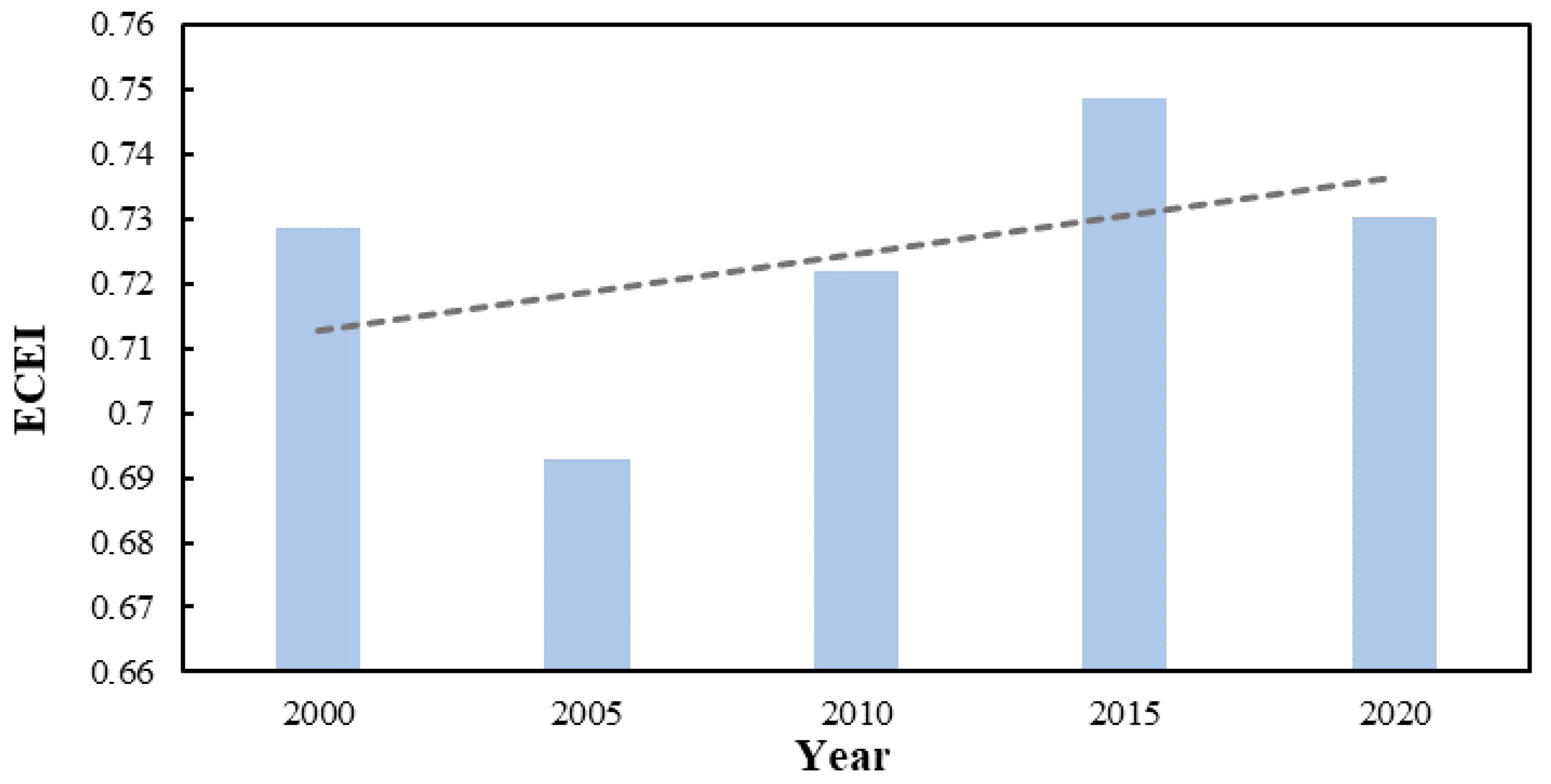
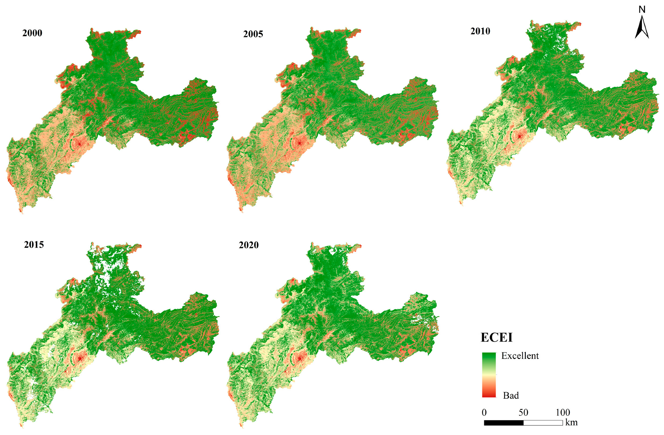
3.1. Spatiotemporal Change Analysis of ECEI

Figure 3 shows the average ECEI values of Zhaotong from 2000 to 2020. Based on Figure 3, all ECEI values in Zhaotong were higher than 0.690, indicating an inverted “N” change trend. In 2005, the ECEI had the lowest value (0.693). In 2015, the ECEI had the highest value (0.749). Generally, the EEQ of Zhaotong has shown an upward trend over the past 20 years, with the ECEI value increasing by 0.23%.
To understand the spatial characteristics of the ECEI, a spatial distribution map at grid and county levels was drawn (Figure 4 and Figure 5).
According to Figure 4, the distribution pattern of EEQ in Zhaotong was relatively stable. Regions located in the northern and eastern parts had high ECEI values. Western areas had moderate ECEI values, better contiguity, and rich patch detail. Areas with low ECEI values showed highly fragmented characteristics. In addition, these regions were mainly distributed in Weixin county, Zhenxiong county, Zhaoyang district, surrounding areas of Shuifu city, Suijiang county, Yongshan county, Daguan county, and Qiaojia county. Except for Chaoyang district, all remaining regions displayed an upward trend to varying degrees. The EEQ of the southern Zhaoyang district was consistent in the past 20 years, with no expansion. In 2015, areas with low ECEI values in Zhaoyang district showed a slight reduction. In addition, the EEQ in the western regions, including Yongshan county, Zhaoyang district, Ludian county, and Qiaojia county, have improved. Due to the lack of satisfying images, in 2015, some regions did not have valid ECEI values. Here, to fully understand the area change with respect to different grades, we set 0.2 as the interval to equally divide ECEI into five grades, which were bad [0,0.2], fair (0.2,0.4], moderate (0.4,0.6], good (0.6,0.8] and excellent (0.8,1]. Table 4 shows the area percentage of different ECEI grades. Figure 6 shows the area percentage bar chart of Zhaotong from 2000 to 2020.
Data from Table 4 and Figure 6 show that the area percentage of different grades in different years was relatively stable. Specifically, for the bad grade, its area percentage displayed an upward trend, with its value increasing from 0.37% in 2000 to 0.73% in 2020. However, the percentage of this grade in all periods was small (lower than 1%). For the fair grade, its area percentage presented a downward change trend, especially in 2020; the area percentage decreased from 13.86% in 2015 to 10.04% in 2020. For the moderate grade, its area percentage increased from 22.39% in 2000 to 23.70% in 2020. For the good grade, its area percentage showed a fluctuating upward trend, with the area percentage rising from 0.57% in 2000 to 7.27% in 2020. As for the excellent grade, its area percentage displayed a fluctuating downward change trend, with the area percentage decreasing from 63.22% in 2000 to 58.26% in 2020. Generally, in 2020, the area percentage of excellent grade decreased. However, the area percentage of moderate, good, and excellent grades in 2020 was the highest. In addition, in all periods, the area percentage of the excellent grade was the highest, indicating that the overall EEQ of Zhaotong city was good.

3.2. Change Direction of ECEI Based on SDE

Figure 7 shows the change direction of ECEI in Zhaotong from 2000 to 2020.
According to Figure 7, the θ range of SDE was from 57.06° to 62.90° with the central areas almost located in the SDE. The distribution pattern of EEQ in Zhaotong presented the direction of “southwest–northeast.” Based on the standard deviation change situation of the major and minor axes of the ellipse, this study was divided into four periods, which were 2000–2005, 2005–2010, 2010–2015, and 2015–2020. Specifically, from 2000 to 2005, the standard deviation of the major and minor axes of the ellipse increased, and regions with high ECEI values moved along the major axis and toward the northeast of Zhaotong city. At the same time, these regions spread toward the minor axis. From 2005 to 2010, the standard deviation of the major and minor axes of the ellipse indicated that the spatial aggregation situation of the ECEI moved toward the gravity center of the ellipse with the coordinate point changing from (386983.50, 3045862.44) to (381051.81, 3041515.11). In general, compared with the previous period, in this period, the changes in southwestern regions’ EEQ played an important role. From 2010 to 2015, standard deviation increments of the major and minor axes of the ellipse were small, and the SDE spatial distribution over two years was similar, indicating that the spatial distribution of EEQ was stable. From 2015 to 2020, standard deviation increments of the major and minor axes of the ellipse were accelerated. Compared with the first period, the transport and expansion intensity were stronger, indicating that the changes in the northeastern regions’ EEQ played an enhanced driving effect. In addition, in this period, the gravity center was located in the northeast corner of Zhaoyang district. In general, from 2000 to 2020, the standard deviation of the major axis of the ellipse moved toward the northeast of Zhaotong city with θ of SDE changing from 57.06° to 62.90°, indicating the improvement of northeastern regions’ EEQ.

3.3. Change Trend of ECEI Based on the Trend Analysis Method

Figure 8 shows the spatial distribution of the ECEI changing trend in Zhaotong from 2000 to 2020.
According to Figure 8, the change trend value ranged from −0.24 to 0.24. Change trend values of most regions were close to 0, indicating that the EEQ of those regions did not show a noticeable improvement or decrease. Regions with low change trend values were mainly distributed in the center of Zhaoyang district. These regions primarily comprised artificial surfaces with intense human activities. To further understand these changes, the center regions of Zhaoyang district were enlarged (b). In Figure 8b, regions with the red color displayed an obvious eco-environmental deterioration. Combined with Figure 8c,d, these regions belonged to urban-expanded areas. In 2021, the urbanization rate of Zhaotong city reached 40.50%, and the build-up area of Zhaoyang district was 62 km2. Other areas with low change trend values presented a scattered distribution. Regions with high change trend values also displayed a scattered distribution. Generally, in the past 20 years, with the increase in urbanization levels, especially the increase in artificial surfaces, the EEQ of the center of Zhaoyang district displayed an evident decrease trend. However, the EEQ’s change trend in most regions of Zhaotong city remained stable, with the change trend value close to 0. Other regions with high or low change trend values showed a scattered distribution.

4. Discussion

4.1. Analysis of ECEI’s SPCA Results

Based on the aforementioned analysis, each ECEI season’s SPCA results were analyzed. Among them, the eigenvalue and percentage of PC1 are shown in Table 5.
According to Table 5, in 2000 and 2005, due to the lack of cloudy-free images, only two seasons were taken into consideration. The eigenvalue represented the information aggregated by the SPCA method. A higher eigenvalue aggregated more information. However, there was no comparison between two or more periods. For example, for the spring–summer season in 2000, the eigenvalue of PC1 was the highest compared with PC2 to PC5. Specifically, for the three remaining periods, four seasons’ cloudy-free images were all available. Specifically, in 2000, the two seasons’ eigenvalues of PC1 were 0.0303 and 0.0292, with PC1 percentages of 73.40% and 80.24%. In 2005, the two seasons’ eigenvalues of PC1 were 0.0325 and 0.0298, with the PC1 percentages of 69.94% and 73.72%. In 2010, four seasons’ eigenvalues of PC1 were 0.0312, 0.0302, 0.0303, and 0.0325, with PC1 percentages of 72.16%, 70.92, 65.83%, and 69.94%. In 2015, four seasons’ eigenvalues of PC1 were 0.0321, 0.0290, 0.0297, and 0.0308, with percentages of 81.47%, 86.93%, 85.43%, and 78.53%. In the year 2020, the eigenvalues of different seasons were 0.0352, 0.0306, 0.0301, and 0.0313, and percentages of PC1 in four seasons were 77.91%, 80.04%, 82.77%, and 79.18%. Generally, the percentages of PC1 were all higher than 65%, with an average percentage value of 76.77%. These results were consistent with the existing RSEI studies. In these studies, even the results of the contribution of PC1 varied. Typically, the contribution was higher than 60% [70,71]. Therefore, based on Table 5, the first component of the SPCA could aggregate the most information of the five indicators, demonstrating the first component’s ability to influence the regional EEQ’s assessment.

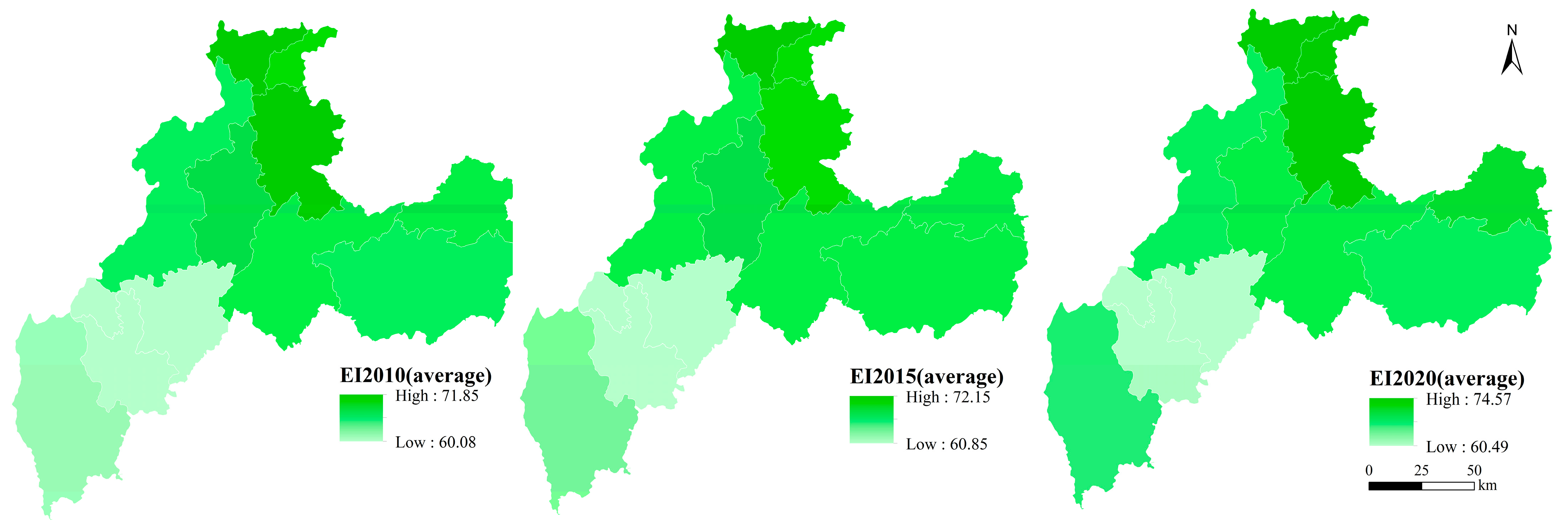
4.2. Validation of ECEI by Comparing with EI

To further validate the effectiveness of the ECEI, the EI was adopted to compare with the ECEI. According to the aforementioned calculation steps, the results of the EI in 2010, 2015, and 2020 were calculated considering the data accessibility. Figure 9 shows the eight sub-indexes calculation results of BI in 2020.
Based on Figure 9, different sub-indexes showed noticeable differences. For WNDI, southern and northwestern Zhaotong had high WNDI values while central regions had low WNDI values, indicating that those regions’ water networks were relatively low. Areas with low HQI values were mainly distributed in Zhaoyang district as those regions had intense human activities. However, the HQI value in northern Zhaotong was relatively high. This is mainly because of those regions’ high vegetation coverage. The spatial distribution of the EVI further validated that areas with high vegetation index are mainly distributed in northern Zhaotong. For SPLIT, regions with high SPLIT values were primarily distributed in southwestern and western parts, indicating that landscape segmentation degrees of these regions were high. However, at the center of Zhaoyang district, the landscape segmentation degree was low. Combined with CONTAG and SIDI, those regions had contiguous artificial surfaces, which further proved that regions with intense human activities usually had low ecosystem and landscape diversity [72,73].
Figure 10 shows the spatial distribution map with the average EI value of Zhaotong city during three periods.
Based on Figure 10, the spatial distribution situation of the average EI during the three periods was similar. Specifically, the average EI values of northern Zhaotong were high, especially in Yanjin and Suijiang counties. However, Zhaoyang district and Ludian county had low average EI values. From the perspective of spatiality, average EI values presented the pattern of high values in the north and low values in the south. From the standpoint of the highest–lowest value, from 2010 to 2020, the lowest values were 60.08, 60.85, and 60.49, respectively, while the highest values were 71.85, 72.15, and 74.57. Generally, the lowest value showed a fluctuating upward trend, with the value increasing by 0.69%. The highest value showed an increasing upward trend with the value increased by 3.78%. These results indicated that the EEQ of Zhaotong improved from 2010 to 2020, which was consistent with the results of the ECEI. In addition, based on the technique criteria, all years’ highest and lowest EI values were higher than 55, indicating that all regions of Zhaotong city qualified for good grades.
To further validate the accuracy of the ECEI, average ECEI and RSEI values of the same three periods were calculated to draw the scatter diagram and establish the fitting curve (Figure 11).
Based on Figure 11, the coefficients of determination (R2) between the EI and ECEI were 0.95 (2010), 0.88 (2015), and 0.89 (2020), with an average R2 of 0.90. As for the R2 between the EI and RSEI, the values of the three periods were 0.31 (2010), 0.92 (2015), and 0.82 (2020), with an average value of 0.69. It could be found that the average R2 value between the EI and ECEI was higher than that of the EI and RSEI, indicating that the ECEI could provide more accurate and scientific EEQ results when considering land surface and season differences. In addition, the R2 of the ECEI was more stable than the RSEI with the value ranging from 0.88 to 0.95, while the R2 of the RSEI went from 0.31 to 0.92. In addition, the R2 of considering all values of the three periods further validated the accuracy of the ECEI with the value of 0.84, which was higher than that of the RSEI (R2 = 0.56). Generally, after considering land surface and season differences, the evaluation of the EEQ in typical cloudy regions was more accurate and scientific compared with the RSEI.

4.3. Implications, Limitations, and Further Study

To evaluate the EEQ of cloudy regions, land surface and season differences were considered to construct a new index-ECEI to assess Zhaotong’s EEQ from 2000 to 2020 accurately and scientifically. Then, the ECEI and RSEI results were compared to validate the effectiveness of the ECEI. Based on the aforementioned analysis, Zhaotong’s EEQ showed a fluctuating upward trend in the past 20 years, with the value increasing from 0.729 to 0.730. From 2000 to 2005, ECEI’s value decreased from 0.729 to 0.693. In this period, due to the rapid population growth and low economic development level, people decided to get more food by destroying forests, cutting trees, and abandoning grazing, thus causing serious water and soil loss and forest coverage loss [72]. From 2002 to 2004, the area of water and soil loss in Zhaotong city increased from 11307.93 km2 to 13362.49 km2 [72,73]. From 2005 to 2020, with the implementation of a series policies, including the “Returning Farmland to Forest (grass) Project”, the forest coverage rate increased from 32.60% in 2011 to 47.80% in 2021. As a result, northern counties had a higher forest coverage rate compared with southern counties. Specifically, Suijiang county’s forest coverage rate reached 71.99% in 2021. In addition, Yanjin, Daguan, Yongshan, and Suijiang counties were listed in the National Key Ecological Function Areas, implemented by the Chinese government since 2007. The number of nature reserves at all levels increased from 8 in 2011 to 23 in 2021, with the area increasing to 1656.00 km2. The controlled area of rocky desertification reached 1180 km2. Moreover, the wastewater treatment rate and garbage harmless treatment rate increased from 41.80% and 45.80% to 98.40% and 100.00%, respectively. Generally, the spatial distribution of the EEQ displayed a pattern of high values in the north and low values in the south, which was consistent with the vegetation coverage situation. Based on the statistical yearbook of Zhaotong, at the end of 2021, the forest coverage rate of Suijiang county was the highest, with a value of 71.99%. Except for Suijiang county and other northern counties in Zhaotong city, forest coverage rates of Yanjin county and Shuifu county were 64.62% and 66.5%. However, the Zhaoyang district’s forest coverage rate was only 38.67%. These results indicated the accuracy of ECEI evaluation results. In addition, the EEQ value of Zhaoyang district was the lowest due to its intense human activities. Existing studies found that human activities could exert a significant influence on the regional EEQ [74,75]. In the future, regions with intense human activities, such as Zhaoyang district, should seek coordinated development between the economy and eco-environment [23].
This paper established the ECEI and evaluated the EEQ of Zhaotong in the past 20 years. Compared with the RSEI, the ECEI results were more accurate and stable. However, this paper still had some limitations. On the one hand, the regional eco-environment belongs to a compound system, including society, economy, and nature [23]. The RSEI only considers four main aspects of the eco-environment. In this study, land surface and season differences were taken into consideration. However, some components, such as air and soil environments, should also be taken into account in the evaluation model. Hence, in further studies, relevant air and soil indicators should be carefully selected to establish a more comprehensive index. On the other hand, for cloudy regions, although the adjacent year was also used to select the satisfying images, this study found that some places did not have any satisfying images. Hence, in further studies, image fusion and image construction from multi-satellites may provide helpful ways to evaluate the regional EEQ thoroughly. Generally, despite these shortcomings, this study still provided a new framework for assessing cloudy regions’ EEQ more accurately and scientifically.

5. Conclusions

Based on multi-source datasets, this study constructed a new eco-environmental comprehensive evaluation index (ECEI) by considering land surface and season differences to evaluate Zhaotong’s EEQ in the past 20 years. Five aspects, such as the biological abundance index (BAI), vegetation cover index (VCI), water network density index (WNDI), land stress index (LSI), and pollution load index (PLI), were also calculated to acquire the ecological index (EI) of Zhaotong at the county level from 2010 to 2020. Finally, spatiotemporal characteristics, standard deviation ellipse (SDE), and trend analysis of Zhaotong’s EEQ at different periods were analyzed. In addition, scatter diagrams of EI–ECEI and EI–RSEI were explored. The main conclusions were as follows: (1) The EEQ of Zhaotong showed a fluctuating upwards trend (0.0058 a−1), with average ECEI values of 0.729, 0.693, 0.722, 0.749, and 0.730. Since 2005, a series of policies, including the “Returning Farmland to Forest (grass) Project”, were implemented to improve Zhaotong’s EEQ. (2) The spatial distribution pattern of EEQ showed high values in the north and low values in the south, which was consistent with the actual forest coverage rate distribution. For example, Suijiang county had a forest coverage rate of 71.99% in 2021. Zhaoyang district had the lowest ECEI value, which was mainly caused by urban sprawl and intense human activities. (3) From 2000 to 2020, the standard deviation of the major axis of the ellipse moved northeast of Zhaotong city with θ of SDE changing from 57.06° to 62.90°, indicating the improvement of northeastern regions’ EEQ; this was related to the increase of National Key Ecological Function Area and nature reserves numbers in northern counties. (4) The coefficients of the determinant (R2) between the EI and ECEI were 0.84, which was higher than that of EI–RSEI (R2 = 0.56). Generally, the ECEI could provide more accurate spatial EEQ evaluation results compared with the RSEI, which could contribute to the regional eco-environmental management, as the spatial pattern of the regional EEQ could be quickly obtained and actual measures could improve the regional EEQ with low ECEI values.

Author Contributions

Conceptualization, J.J.; methodology, L.J. and Z.T.; software, L.J. and T.S.; validation, F.Z., L.J. and R.Z.; formal analysis, L.J.; investigation, E.S.; resources, W.L., H.L. (Huan Li), X.L. and H.L. (Huiyuan Lu); data curation, L.J.; writing—original draft preparation, J.J. and L.J.; writing—review and editing, J.J. and E.S.; visualization, R.Z.; supervision, W.L.; project administration, J.J.; funding acquisition, J.J. All authors have read and agreed to the published version of the manuscript.

Funding

This research was funded by the Humanities and Social Sciences Foundation of Suzhou University of Science and Technology (No. XKR202102), Philosophy and Social Science Research in Colleges and Universities of Jiangsu Province (No. 2022SJYB1465), Starting Research Program of Suzhou University of Science and Technology (No. 332114809) and the Jiangsu University Students Innovation and Entrepreneurship Training Program Fund Project (No. 202210332073Y).

Institutional Review Board Statement

Not applicable.

Informed Consent Statement

Not applicable.

Data Availability Statement

The data presented in this study are available on request from the corresponding author.

Acknowledgments

We thank the Google Earth Engine platform, National Aeronautics and Space Administration, United States Geological Survey, Geospatial Data Cloud, Data Sharing and Service Portal, National Earth System Science Data Center, Food and Agriculture Organization of the United Nations, National Geomatics Center of China, and Jing Wei for supplying the administrative division data and remote sensing datasets.

Conflicts of Interest

The authors declare no conflict of interest.

Abbreviations

AIAbundance indexAn index for describing regional biological abundance
BIBiodiversity indexAn index for describing regional biodiversity
ECEIEco-environmental comprehensive evaluation indexAn index for evaluating regional comprehensive eco-environmental quality
EEQEco-environmental qualityA measure of regional eco-environmental quality
EIEcological indexAn index for describing ecological quality
GEEGoogle Earth EngineA cloud platform for processing massive data
HQIHabitat quality indexAn index for describing regional habitat quality
LSILand stress indexAn index for describing regional land stress
LSTLand surface temperatureAn index for describing regional eco-environmental heat
NDBSINormalized difference build-up and soil indexAn index for describing regional eco-environmental dryness
NDVINormalized difference vegetation indexAn index for describing regional eco-environmental greenness
RSEIRemote sensing ecological indexAn index for describing eco-environmental quality
SDEStandard deviation ellipseAn ellipse for measuring the standard deviation of data
SPCASpatial principal component analysisA multivariate statistical analysis method
WETWetnessAn index for describing regional eco-environmental wetness
WNDIWater network density indexAn index for describing regional water network density

References

  1. Zhang, X.; Song, W.; Wang, J.; Wen, B.; Yang, D.; Jiang, S.; Wu, Y. Analysis on decoupling between urbanization level and urbanization quality in China. Sustainability 2020, 12, 6835. [Google Scholar] [CrossRef]
  2. United Nations. World Urbanization Prospects: The 2013 Revision; United Nations: New York, NY, USA, 2014. [Google Scholar]
  3. National Bureau of Statistics of the People’s Republic of China. China Statistical Yearbook (2022); China Statistics Press: Beijing, China, 2022.
  4. Zhao, G.; Mu, X.; Wen, Z.; Wang, F.; Gao, P. Soil erosion, conservation, and eco-environment changes in the Loess plateau of China. Land Degrad. Develop. 2013, 24, 499–510. [Google Scholar] [CrossRef]
  5. Rao, E.; Xiao, Y.; Ouyang, Z.; Yu, X. National assessment of soil erosion and its spatial patterns in China. Ecosyst. Health Sust. 2015, 1, 1–10. [Google Scholar] [CrossRef]
  6. Pennekamp, F.; Pontarp, M.; Tabi, A.; Altermatt, F.; Alther, R.; Choffat, Y.; Fronhofer, E.; Ganesanandamoorthy, P.; Garnier, A.; Griffiths, J.; et al. Biodiversity increases and decreases ecosystem stability. Nature 2018, 563, 109–112. [Google Scholar] [CrossRef] [Green Version]
  7. Hao, J.; Xu, G.; Luo, L.; Zhang, Z.; Yang, H.; Li, H. Quantifying the relative contribution of natural and human factors to vegetation coverage variation in coastal wetlands in China. Catena 2020, 188, 104429. [Google Scholar] [CrossRef]
  8. Estoque, R.C.; Murayama, Y.; Myint, S.W. Effects of landscape composition and pattern on land surface temperature: An urban heat island study in the megacities of southeast Asia. Sci. Total Environ. 2017, 577, 349–359. [Google Scholar] [CrossRef]
  9. Geng, X.; Zhang, D.; Li, C.; Yuan, Y.; Yu, Z.; Wang, X. Impacts of climate zones on urban heat island: Spatiotemporal variations, trends, and drivers in China from 2001-2020. Sustain. Cities Soc. 2023, 89, 104303. [Google Scholar] [CrossRef]
  10. Dey, S.; Girolamo, L.D.; Donkelaar, A.; Tripathi, S.N.; Gupta, T.; Mohan, M. Variability of outdoor fine particulate (PM2.5) concentration in the Indian subcontinent: A remote sensing approach. Remote Sens. Environ. 2012, 127, 153–161. [Google Scholar] [CrossRef]
  11. Liu, M.; Bi, J.; Ma, Z. Visibility-based PM2.5 concentrations in China: 1957-1964 and 1973-2014. Environ. Sci. Technol. 2017, 51, 13161–13169. [Google Scholar] [CrossRef]
  12. Hu, S.; Yang, Y.; Zheng, H.; Mi, C.; Ma, T.; Shi, R. A framework for assessing sustainable agriculture and rural development: A case study of the Beijing-Tianjin-Hebei region, China. Environ. Impact Asses. 2022, 97, 106861. [Google Scholar] [CrossRef]
  13. Ji, J.; Wang, S.; Zhou, Y.; Liu, W.; Wang, L. Spatiotemporal Change and Coordinated Development Analysis of “PopulationSociety-Economy-Resource-Ecology-Environment” in the Jing-Jin-Ji Urban Agglomeration from 2000 to 2015. Sustainability 2021, 13, 4075. [Google Scholar] [CrossRef]
  14. Marando, F.; Heris, M.; Zuilian, G.; Udías, A.; Mentaschi, L.; Chrysoulakis, N.; Parastatidis, D.; Maes, J. Urban heat island mitigation by green infrastructure in European Functional Urban Areas. Sustain. Cities Soc. 2022, 77, 103564. [Google Scholar] [CrossRef]
  15. Donati, G.; Bolliger, J.; Psomas, A.; Maurer, M.; Bach, P. Reconciling cities with nature: Identifying local blue-green infrastructure interventions for regional biodiversity enhancement. J. Environ. Manag. 2022, 316, 115254. [Google Scholar] [CrossRef] [PubMed]
  16. Chanchitpricha, C.; Fischer, T. The role of impact assessment in the development of urban green infrastructure: A review of EIA and SEA practices in Thailand. Impact Assess. Proj. A. 2022, 40, 191–201. [Google Scholar] [CrossRef]
  17. Barbosa, V.; Pradilla, M.; Chica-Mejía, J.; Bonilla, J. Functionality and Value of Green Infrastructure in Metropolitan Sprawl: What Is the City’s Future? A Case Study of the Bogotá-Sabana Northern Region; IntechOpen: London, UK, 2022. [Google Scholar]
  18. Ewing, R.; Hamidi, S. Compactness versus sprawl: A review of recent evidence from the United States. J. Plan. Lit. 2015, 30, 413–432. [Google Scholar] [CrossRef]
  19. Polidoro, M.; Lollo, J.; Barros, M. Urban sprawl and the challenges for urban planning. J. Environ. Prot. 2012, 3, 1010–1019. [Google Scholar] [CrossRef] [Green Version]
  20. Tian, L.; Li, Y.; Yan, Y.; Wang, B. Measuring urban sprawl and exploring the role planning plays: A Shanghai case study. Land Use Policy 2017, 67, 426–435. [Google Scholar] [CrossRef]
  21. Huang, S.; Wang, S.; Budd, W. Sprawl in Taipei’s peri-urban zone: Responses to spatial planning and implications for adapting global environmental change. Landscape Urban Plan. 2009, 90, 20–32. [Google Scholar] [CrossRef]
  22. Barbosa, V.; Pradilla, M. Identifying the social urban spatial structure of vulnerability: Towards climate change equity in Bogotá. Urban Plan. 2021, 6, 365–379. [Google Scholar] [CrossRef]
  23. Ji, J.; Tang, Z.; Zhang, W.; Liu, W.; Jin, B.; Xi, X.; Wang, F.; Zhang, R.; Guo, B.; Xu, Z.; et al. Spatiotemporal and multiscale analysis of the coupling coordination degree between economic development equality and eco-environmental quality in China from 2001 to 2020. Remote Sens. 2022, 14, 737. [Google Scholar] [CrossRef]
  24. Ji, J.; Wang, S.; Zhou, Y.; Liu, W.; Wang, L. Studying the Eco-Environmental Quality Variations of Jing-Jin-Ji Urban Agglomeration and Its Driving Factors in Different Ecosystem Service Regions From 2001 To 2015. IEEE Access 2020, 8, 154940–154952. [Google Scholar] [CrossRef]
  25. Fu, B. The evaluation of eco-environmental qualities in China. China Popul. Resour. Environ. 1992, 2, 48–54. (In Chinese) [Google Scholar]
  26. He, C.; Gao, B.; Huang, Q.; Ma, Q.; Dou, Y. Environmental degradation in the urban areas of China: Evidence from multi-source remote sensing data. Remote Sens. Environ. 2017, 193, 65–75. [Google Scholar] [CrossRef]
  27. Wei, W.; Guo, Z.; Xie, B.; Zhou, J.; Li, C. Spatiotemporal evolution of environment based on integrated remote sensing indexes in arid inland river basin in Northwest China. Environ. Sci. Pollut. Res. 2019, 26, 13062–13084. [Google Scholar] [CrossRef]
  28. Chang, Y.; Hou, K.; Wu, Y.; Li, X.; Zhang, J. A conceptual framework for establishing the index system of ecological environment evaluation-A case study of the upper Hanjiang River, China. Ecol. Indic. 2019, 107, 105568. [Google Scholar] [CrossRef]
  29. Sun, R.; Wu, Z.; Chen, B.; Yang, C.; Qi, D.; Lan, G.; Fraedrich, K. Effects of land-use change on eco-environmental quality in Hainan Island, China. Ecol. Indic. 2020, 109, 105777. [Google Scholar] [CrossRef]
  30. Wei, W.; Shi, S.; Zhang, X.; Zhou, L.; Xie, B.; Zhou, J.; Li, C. Regional-scale assessment of environmental vulnerability in an arid inland basin. Ecol. Indic. 2020, 109, 105792. [Google Scholar] [CrossRef]
  31. Chai, L.; Lha, D. A new approach of deriving indicators and comprehensive measure for ecological environmental quality assessment. Ecol. Indic. 2018, 85, 716–728. [Google Scholar] [CrossRef]
  32. Ariken, M.; Zhang, F.; Chan, N.; Kung, H. Coupling coordination analysis and spatio-temporal heterogeneity between urbanization and eco-environment along the Silk Road Economic Belt in China. Ecol. Indic. 2021, 121, 107014. [Google Scholar] [CrossRef]
  33. Huang, Y.; Qiu, Q.; Sheng, Y.; Min, X.; Cao, Y. Exploring the Relationship between Urbanization and the Eco-Environment: A Case Study of Beijing. Sustainability 2019, 11, 6298. [Google Scholar] [CrossRef] [Green Version]
  34. Yu, Q.; Ji, J.; Zhang, R.; Liu, W. Spatiotemporal evolution of coupling coordination level between eco-environment and economy based on multi-source data: A case study of Jing-Jin-Ji urban agglomeration. J. Safety Environ. 2022, 20, 3541–3549. (In Chinese) [Google Scholar]
  35. Ji, J.; Tang, Z.; Wang, L.; Liu, W.; Eshetu, S.; Zhang, W.; Guo, B. Spatiotemporal Analysis of the Coupling Coordination Degree between Haze Disaster and Urbanization Systems in China from 2000 to 2020. Systems 2022, 10, 150. [Google Scholar] [CrossRef]
  36. Yang, Q.; Liu, X.; Huang, Z.; Guo, B.; Tian, L.; Wei, C.; Meng, Y.; Zhang, Y. Integrating satellite-based passive microwave and optically sensed observations to evaluating the spatio-temporal dynamics of vegetation health in the red soil regions of southern China. Gisci. Remote Sens. 2022, 59, 215–233. [Google Scholar] [CrossRef]
  37. Li, K.; Chen, Y. Identifying and characterizing frequency and maximum durations of surface urban heat and cool island across global cities. Sci. Total. Environ. 2022, 859, 160218. [Google Scholar] [CrossRef]
  38. Ji, J.; Wang, S.; Zhou, Y.; Liu, W.; Wang, L. Spatiotemporal change and landscape pattern variation of eco-environmental quality in Jing-Jin-Ji urban agglomeration from 2001 to 2015. IEEE Access 2020, 8, 125534–125548. [Google Scholar] [CrossRef]
  39. Xu, H. A remote sensing urban ecological index and its application. Acta Ecol. Sinica. 2013, 33, 7853–7862. (In Chinese) [Google Scholar]
  40. Lin, L.; Hao, Z.; Post, C.; Mikhailova, E. Monitoring Ecological Changes on a Rapidly Urbanizing Island Using a Remote Sensing-Based Ecological Index Produced Time Series. Remote Sens. 2022, 14, 5773. [Google Scholar] [CrossRef]
  41. Yang, Z.; Sun, C.; Ye, J.; Gan, C.; Li, Y.; Wang, L.; Chen, Y. Spatio-Temporal Heterogeneity of Ecological Quality in Hangzhou Greater Bay Area (HGBA) of China and Response to Land Use and Cover Change. Remote Sens. 2022, 14, 5613. [Google Scholar] [CrossRef]
  42. Wang, J.; Ding, J.; Ge, X.; Qin, S.; Zhang, Z. Assessment of ecological quality in Northwest China (2000-2020) using the Google Earth Engine platform: Climate factors and land use/land cover contribute to ecological quality. J. Arid Land 2022, 14, 1196–1211. [Google Scholar] [CrossRef]
  43. Yang, X.; Meng, F.; Fu, P.; Zhang, Y.; Liu, Y. Spatiotemporal change and driving factors of the Eco-Environment quality in the Yangtze River Basin from 2001 to 2019. Ecol. Indic. 2021, 131, 108214. [Google Scholar] [CrossRef]
  44. Xu, D.; Cheng, J.; Xu, S.; Geng, J.; Yang, F.; Fang, H.; Xu, J.; Wang, S.; Wang, Y.; Huang, J.; et al. Understanding the Relationship between China’s Eco-Environmental Quality and Urbanization Using Multisource Remote Sensing Data. Remote Sens. 2022, 14, 198. [Google Scholar] [CrossRef]
  45. Xu, D.; Yang, F.; Yu, L.; Zhou, Y.; Li, H.; Ma, J.; Huang, J.; Wei, J.; Xu, Y.; Zhang, C.; et al. Quantization of the coupling mechanism between eco-environmental quality and urbanization from multisource remote sensing data. J. Clean Prod. 2021, 321, 128948. [Google Scholar] [CrossRef]
  46. Zhang, T.; Yang, R.; Yang, Y.; Li, L.; Chen, L. Assessing the Urban Eco-Environmental Quality by the Remote-Sensing Ecological Index: Application to Tianjin, North China. ISPRS Int. J. Geo-Inf. 2021, 10, 475. [Google Scholar] [CrossRef]
  47. Xu, H.; Deng, W. Rationality Analysis of MRSEI and Its Difference with RSEI. Remote Sens. Technol. Appl. 2022, 37, 1–7. (In Chinese) [Google Scholar]
  48. Liu, Z.; Wang, L.; Li, B. Quality Assessment of Ecological Environment Based on Google Earth Engine: A Case Study of the Zhoushan Islands. Front. Ecol. Evol. 2022, 10, 918756. [Google Scholar] [CrossRef]
  49. Xia, X.; Jiao, C.; Song, S.; Zhang, L.; Feng, X.; Huang, Q. Developing a method for assessing environmental sustainability based on the Google Earth Engine platform. Environ. Sci. Pollut. Res. 2022, 29, 57437–57452. [Google Scholar] [CrossRef]
  50. Zhang, M.; He, T.; Wu, C.; Li, G. The Spatiotemporal Changes in Ecological-Environmental Quality Caused by Farmland Consolidation Using Google Earth Engine: A Case Study from Liaoning Province in China. Remote Sens. 2022, 14, 3646. [Google Scholar] [CrossRef]
  51. Liu, Y.; Luo, K.; Li, L.; Shahid, M. Fluoride and sulfur dioxide indoor pollution situation and control in coal-burning endemic area in Zhaotong, Yunnan, China. Atmos. Environ. 2013, 77, 725–737. [Google Scholar] [CrossRef]
  52. Yunnan Provincial Bureau of Statistics. Yunnan Statistical Yearbook (2021); China Statistics Press: Beijing, China, 2021.
  53. Li, Y.; Chang, C.; Wang, Z.; Zhao, G. Remote sensing prediction and characteristic analysis of cultivated land salinization in different seasons and multiple soil layers in the coastal area. Int. J. Appl. Earth Obs. 2022, 111, 102838. [Google Scholar] [CrossRef]
  54. Ye, X.; Kuang, H. Evaluation of ecological quality in southeast Chongqing based on modified remote sensing ecological index. Sci. Rep. 2022, 12, 15694. [Google Scholar] [CrossRef]
  55. Zhu, D.; Chen, T.; Wang, Z.; Niu, R. Detecting ecological spatial-temporal changes by Remote Sensing Ecological Index with local adaptability. J. Environ. Manag. 2021, 299, 113655. [Google Scholar] [CrossRef] [PubMed]
  56. Joshi, P.; Wynne, R.; Thomas, V. Cloud detection algorithm using SVM with SWIR2 and tasseled cap applied to Landsat 8. Int. J. Appl. Earth Obs. 2019, 82, 101898. [Google Scholar] [CrossRef]
  57. Liu, Q.; Liu, G.; Huang, C.; Xie, C.; Chu, L.; Shi, L. Comparison of tasselled cap components of images from Landsat 5 Thematic Mapper and Landsat 7 Enhanced Thematic Mapper Plus. J. Spat. Sci. 2016, 61, 351–365. [Google Scholar] [CrossRef]
  58. Technical Criterion for Ecosystem Status Evaluation, Document, HJ 192–2015. 2015. Available online: https://www.mee.gov.cn/ywgz/fgbz/bz/bzwb/stzl/201503/t20150324_298011.shtml (accessed on 2 September 2022).
  59. Gatti, R.; Notarnicola, C. A novel Multilevel Biodiversity Index (MBI) for combined field and satellite imagery surveys. Glob. Ecol. Conserve. 2018, 13, e00361. [Google Scholar] [CrossRef]
  60. Qie, G.; Lin, W.; Xu, R.; Li, L. Calculation and Analysis of SDG 15.1.2 Biodiversity Index Based on Remote Sensing: A Case Study of Demonstration Zone of Green and Integrated Ecological Development of the Yangtze River Delta. Res. Environ. Sci. 2022, 35, 1025–1036. (In Chinese) [Google Scholar]
  61. Wang, B.; Cheng, W. Effects of Land Use/Cover on Regional Habitat Quality under Different Geomorphic Types Based on InVEST Model. Remote Sens. 2022, 14, 1279. [Google Scholar] [CrossRef]
  62. Li, M.; Zhou, Y.; Xiao, P.; Tian, Y.; Huang, H.; Xiao, L. Evolution of Habitat Quality and Its Topographic Gradient Effect in Northwest Hubei Province from 2000 to 2020 Based on the InVEST Model. Land 2021, 10, 857. [Google Scholar] [CrossRef]
  63. Yousif, M.; Sracek, O. Integration of geological investigations with multi-GIS data layers for water resources assessment in arid regions: EI Ambagi Basin, Eastern Desert, Egypt. Environ. Earth Sci. 2016, 75, 684. [Google Scholar] [CrossRef]
  64. Wei, J.; Liu, S.; Li, Z.; Liu, C.; Qin, K.; Liu, X.; Pinker, R.; Dickerson, R.; Lin, J.; Boersma, K.; et al. Ground-level NO2 surveillance from space across China for high resolution using interpretable spatiotemporally weighted artificial intelligence. Environ. Sci. Technol. 2022, 56, 9988–9998. [Google Scholar] [CrossRef]
  65. Wei, J.; Li, Z.; Lyapustin, A.; Sun, L.; Peng, Y.; Xue, W.; Su, T.; Cribb, M. Reconstructing 1-km-resolution high-quality PM2.5 data records from 2000 to 2018 in China: Spatiotemporal variations and policy implications. Remote Sens. Environ. 2021, 252, 112136. [Google Scholar] [CrossRef]
  66. Xiong, J.; Ye, C.; Cheng, W.; Guo, L.; Zhou, C.; Zhang, X. The Spatiotemporal Distribution of Flash Floods and Analysis of Partition Driving Forces in Yunnan Province. Sustainability 2019, 11, 2926. [Google Scholar] [CrossRef] [Green Version]
  67. Wang, B.; Shi, W.; Miao, Z. Confidence Analysis of Standard Deviational Ellipse and Its Extension into Higher Dimensional Euclidean Space. PLoS One 2015, 10, e0118537. [Google Scholar] [CrossRef] [PubMed]
  68. Xu, J. Mathematical Methods in Contemporary Geography, 2nd ed.; Higher Education Press: Beijing, China, 2002. (In Chinese) [Google Scholar]
  69. Zhao, H.; Chen, Y.; Zhou, Y.; Pei, T.; Xie, B.; Wang, X. Spatiotemporal variation of NDVI in vegetation growing season and its responses to climate factors in mid and eastern Gansu Province from 2008 to 2016. Arid Land Geogra. 2019, 42, 1427–1435. (In Chinese) [Google Scholar]
  70. Gao, W.; Zhang, S.; Rao, X.; Lin, X.; Li, R. Landsat TM/OLI-Based Ecological and Environmental Quality Survey of Yellow River Basin, Inner Mongolia Section. Remote Sens. 2021, 13, 4477. [Google Scholar] [CrossRef]
  71. Xiong, Y.; Xu, W.; Lu, N.; Huang, S.; Wu, C.; Wang, L.; Dai, F.; Kou, W. Assessment of spatial–temporal changes of ecological environment quality based on RSEI and GEE: A case study in Erhai Lake Basin, Yunnan province, China. Ecol. Indic. 2021, 125, 107518. [Google Scholar] [CrossRef]
  72. Wang, Y. A demonstration analysis on the mountainous region on the south west of China for economic development and its ecological protection—The case of Zhaotong in Yunnan province. Yunnan Geogra. Environ. Researh 2004, 7, 47–50. (In Chinese) [Google Scholar]
  73. Jiang, C. Eco-environment of Zhaotong prefecture and countermeasures for problems. Environ. Sci. Survey 2002, 21, 29–31. (In Chinese) [Google Scholar]
  74. Hong, G.; Chi, W.; Pan, T.; Dou, Y.; Kuang, W.; Guo, C.; Hao, R.; Bao, Y. Examining Spatio-Temporal Dynamics of Ecological Quality in the Pan-Third Pole Region in the Past 20 years. Remote Sens. 2022, 14, 5473. [Google Scholar] [CrossRef]
  75. Kuang, W.; Liu, J.; Tian, H.; Shi, H.; Dong, J.; Song, C.; Li, X.; Du, G.; Hou, Y.; Lu, D.; et al. Cropland redistribution to marginal lands undermines environmental sustainability. Natl. Sci. Rev. 2022, 9, nwab091. [Google Scholar] [CrossRef]
Figure 1. Location of the study area.
Remotesensing 15 00657 g001
Figure 2. Framework of this study.
Remotesensing 15 00657 g002
Figure 3. Average ECEI values of Zhaotong from 2000 to 2020.
Remotesensing 15 00657 g003
Figure 4. Spatial distribution of ECEI in Zhaotong from 2000 to 2020.
Remotesensing 15 00657 g004
Figure 5. Spatial distribution of ECEI in Zhaotong from 2000 to 2020 at the county level.
Remotesensing 15 00657 g005
Figure 6. Average ECEI values of Zhaotong from 2000 to 2020.
Remotesensing 15 00657 g006
Figure 7. Change direction in Zhaotong from 2000 to 2020.
Remotesensing 15 00657 g007
Figure 8. Spatial distribution of the changing trend of ECEI from 2000 to 2020 (a), change trend of the selected region (b), Landsat image in 2005 (c), and Landsat image in 2020 (d).
Remotesensing 15 00657 g008
Figure 9. Eight sub-indexes calculation results of BI in 2020.
Remotesensing 15 00657 g009
Figure 10. Spatial distribution map of average EI value from 2010 to 2020.
Remotesensing 15 00657 g010
Figure 11. Scatter diagram of EI, RSEI, and ECEI from 2010 to 2020.
Remotesensing 15 00657 g011
Table 1. Brief introduction of datasets.
NameResolutionData AvailabilityBrief Description
Landsat series30 mhttps://www.usgs.gov/landsat-missions/landsat-collection-2-level-2-science-products
accessed on 1 May 2022
A product of land surface spectral reflectance
GLC_FCS3030 mhttps://data.casearth.cn/
accessed on 15 May 2022
A product of global land cover with fine classification system
ASTER GDEM30 mhttp://www.gscloud.cn/home
accessed on 22 May 2022
A product of global digital elevation model
Precipitation1000 mhttp://www.geodata.cn
accessed on 5 July 2022
A product of monthly precipitation data
CHAP1000 mhttps://weijing-rs.github.io/product.html
accessed on 20 June 2022
Products of China’s high-spatial air pollutants
HWSD30 arc-secondhttps://www.fao.org/soils-portal/soil-survey/soil-maps-and-databases/harmonized-world-soil-database-v12/en/
accessed on 20 June 2022
A product of harmonized world soil database
Statistical yearbook\http://www.zt.gov.cn/
accessed on 20 June 2022
Statistical data of regional socio-economic aspects
Administrative boundary data\http://www.ngcc.cn/ngcc/html/1/index.html
accessed on 5 May 2022
A vector dataset for data mask and spatial analysis
Table 2. Weight and sub-indicator system of BI.
LevelWeightSub-IndicatorWeight
Species diversity0.60Habitat quality index (HQI)0.30
Enhanced vegetation index (EVI)0.15
Water network density index (WNDI)0.15
Ecosystem diversity0.15Percentage of habitat area (Sp)0.05
Simpson diversity index (SIDI)0.10
Landscape diversity0.25Splitting index (SPLIT)0.15
Contagion index (CONTAG)0.10
Table 3. Pollutant allocation indicator system.
Target LevelElement LayerIndicatorWeight
Pollutant emissions allocationEnvironmentWater quality (WQ)0.38
EconomyGross domestic product (GRP)0.33
SocietyPopulation density (PD)0.29
Table 4. Area percentage of different ECEI grades.
ECEI Grades20002005201020152020
Area
Percentage/%
Area
Percentage/%
Area
Percentage/%
Area
Percentage/%
Area
Percentage/%
Bad0.370.490.610.790.73
Fair13.4513.4813.4813.8610.04
Moderate22.3922.3122.3622.4423.70
Good0.572.650.590.637.27
Excellent63.2261.0762.9662.2858.26
Table 5. Each ECEI season’s SPCA results.
YearSeasonEigenvalue of PC1Percentage of PC1/%
2000Spring–Summer0.030373.40
Autumn–Winter0.029280.24
2005Spring–Summer0.032569.94
Autumn–Winter0.029873.72
2010Spring0.031272.16
Summer0.030270.92
Autumn0.030365.83
Winter0.032569.94
2015Spring0.032181.47
Summer0.029086.93
Autumn0.029785.43
Winter0.030878.53
2020Spring0.035277.91
Summer0.030680.04
Autumn0.030182.77
Winter0.031379.18
Disclaimer/Publisher’s Note: The statements, opinions and data contained in all publications are solely those of the individual author(s) and contributor(s) and not of MDPI and/or the editor(s). MDPI and/or the editor(s) disclaim responsibility for any injury to people or property resulting from any ideas, methods, instructions or products referred to in the content.

