Usage of Airborne LiDAR Data and High-Resolution Remote Sensing Images in Implementing the Smart City Concept

Abstract

The cities of the future should not only be smart, but also smart green, for the well-being of their inhabitants, the biodiversity of their ecosystems and for greater resilience to climate change. In a smart green city, the location of urban green spaces should be based on an analysis of the ecosystem services they provide. Therefore, it is necessary to develop appropriate information technology tools that process data from different sources to support the decision-making process by analysing ecosystem services. This article presents the methodology used to develop an urban green space planning tool, including its main challenges and solutions. Based on the integration of data from ALS, CLMS, topographic data, and orthoimagery, an urban green cover model and a 3D tree model were generated to complement a smart-city model with comprehensive statistics. The applied computational algorithms allow for reports on canopy volume, CO${}_2$ reduction, air pollutants, the effect of greenery on average temperature, interception, precipitation absorption, and changes in biomass. Furthermore, the tool can be used to analyse potential opportunities to modify the location of urban green spaces and their impact on ecosystem services. It can also assist urban planners in their decision-making process.

1. Introduction

The development of green, healthy, and attractive cities should take a holistic approach to environmental issues and the production and management of energy from traditional and renewable sources, supported by environmental and climate knowledge. The spaces designated for green and blue infrastructure in cities must be seen, not only as an investment area, but also as a valuable asset. The arrangement of green spaces in the city is as important as their amount and accessibility. This includes the size and distribution, as well as the location and proximity to residential areas, in order to benefit biodiversity and human health [1,2]. Numerous studies have been conducted on the use of UGS (urban green spaces) as a result of the COVID-19 pandemic, which strongly influenced the public perception of urban greenery [3,4]—the pandemic affected both the purpose of visiting (from collective to individual) and the choice of available green spaces; additionally, access to urban green spaces was considered essential for health [5]. These studies provided a great amount of information on the behaviour and needs of urban residents, helping urban planners provide public access to green areas [6,7,8], taking into account the different needs of social groups and their spatial distribution. For this purpose, urban planners use tools such as participatory mapping or online surveys [9]. However, surveys that focus solely on human preferences are insufficient for planning UGS, as they are an essential part of the city’s ecosystem.

Other problems can also be encountered: it can be observed that when determining the impact of green areas on the ecology of the city, the impact of green areas of private property is sometimes underestimated, mainly due to a lack of information (e.g., land use, vegetation inventory, and classification of existing greenery species) [10,11]. A detailed inventory of green areas is often limited to green areas under governmental management (inventoried in their databases). For other spaces, the problem is determining the ratio of the number of trees to the area, as well as the volume of tree crowns, as their layout may be compact or dispersed. Some of these issues can be solved using remote sensing tools. In addition, other problems can also be encountered. For example, the use of unmanned aerial vehicles (UAVs) can be problematic due to the need for permits and the dilution of the point cloud at higher altitudes [12]. Furthermore, aerial and satellite imagery does not provide information on tree heights, and tree crowns are not always distinguished from other groups of objects in the image [13]. Another limitation of UGS information is the simplifications assumed; in the popular V-I-S (vegetation–impervious surface–soil) model, the urban landscape is considered as the simple sum of vegetation, impervious surfaces, and soil. This model does not make a distinction between trees and other forms of vegetation. Other methods are very time-consuming and cost-consuming, with relatively low accuracy. With the presence of more vegetation forms, most methods do not take into account that canopy cover varies throughout the year [2].

Automatic assignment of land cover in a city is a complex task, requiring additional databases that take into account time variation and spatial uncertainty, due to the high variability and coexistence of green infrastructure with other forms of land cover (e.g., trees along streets). Methods for determining tree parameters often use artificial intelligence in combination with one or more data sources [14], such as satellite imagery and light detection and ranging (LiDAR) data sets [15], neural networks to automatically classify forest LiDAR point cloud [16], UAVs, Google street view [17,18], or images taken with smartphones [12].

The type and resolution of the data used often depend on the scale of the analysis. It is becoming increasingly popular to depart from the distinction between the ‘in the city’ approach, which considers green spaces as part of the urban space, and the ecology ‘of the city’ treating the city as a total [2]. Nowadays, thanks to the use of Geographic Information Systems (GIS) and remote sensing tools, these methods can be combined and cities can be treated as integrated social-ecological systems, allowing us to learn about the impact of small-scale phenomena on city-wide processes. This approach requires appropriate parameter unification methods to allow for transitions between scales and the use of different sensors to acquire information on different scales [19]. Design focused on general information and percentage canopy cover lacks a ‘more than human’ tree-orientated approach that could lead to the creation of ‘smart urban forests’ [20] as part of the concept of smart cities. The concept of smart cities is a coherent system that operates on the basis of information and communication technologies (ICT), monitoring, automation, and computer technologies. This also allows for interaction between city officials and the community, aiming to improve the quality of city services [21]. Furthermore, to achieve the status of a smart city, the city must have all the characteristics of a smart environment [22,23], as shown in Figure 1.

Urban green management issues in the smart city can be divided into two main groups [24]: (i) one that assumes the use of digital technologies such as wireless networks, sensors, and cloud-based storage to improve the ecosystem services of green infrastructure and to improve the ability to observe and collect information about green spaces and their functioning, and (ii) another that assumes the participation of citizens and businesses in urban green management through open mapping platform services, volunteered geographic information (VGI) initiatives, and social networks, in line with the concept ‘Smart City 3.0’, which is the most sustainable vision of the smart city that extends the range of needs to include software and solutions that involve residents in urban management [25,26].

The integration of smart city and green city concepts requires the consideration of many variables related to the ecosystem and cultural services of urban green spaces, which generate the need for tools for different levels of management [27]. Specialised analyses of the impact of green spaces on the spatial planning process are not always possible due to the costs and time involved. Local authorities need simple, fast, and credible decision-support tools to optimise the location and use of urban green spaces. Recent tools developed to support the design and management of urban green spaces include the Nature Smart Cities Business Model (NSC-BM) [27], which aims to help authorities of smaller municipalities to assess the potential impact of a green infrastructure project in the early planning stages, based on user input of the parameters of the project under consideration. Another approach introduces a tool that uses urban green mapping and composite benefit scores for given areas, developed based on a multi-criteria analysis, as a tool to support urban green location planning in regions with rapid urbanisation [28]. Another example of the use of different types of multi-criteria analysis for the allocation of green infrastructure (GI) is the evaluation of different approaches, such as the opinion of environmental, social, and financial groups [29].

The methodology presented in this paper is a contribution to the SekoZ project (Polish acronym that stands for the System Ewaluacji Usług Ekosystemowych Zieleni Mieskiej, the service system for the evaluation of green urban ecosystems), which is a comprehensive, unexplored, and innovative decision-support tool for the location of urban green spaces in cities of different sizes, based on indicators that quantify urban green ecosystem services and the impacts of land use modification on the city scale. This tool addresses one of the main challenges in the quantification of ecosystem services provided by trees, which has been the automatic inventory and generation of stand geometry for the determination of ecosystem service indicators.

2. Materials and Methods

2.1. Area of the Study

The test area and the pilot site for the SekoZ project was Poznań, a major city in Poland, located in the western part of the country (see Figure 2), between Warsaw and Berlin. Poznań, as the capital of the Greater Poland Voivodeship, is a prominent economic, cultural, and scientific hub in both the region and the country.

It has an area of 261.9 km${}^2$ and its administrative boundaries extend about 22 km from north to south and 21 km from east to west. Every day, Poznań’s urban space is used by about 700,000 people: permanent and temporary residents, as well as tourists and professionals. In 2021, its green areas, including 52 publicly accessible parks and 123 green spaces, represented 27% of the city’s territory (for a more detailed summary, see

Table 1. Covered land use area within the territory of Poznań city.

Land Use	Area (km${}^2$)	Area (%)
Forrest	43.79	16.72
Other greenery	20.84	7.95
Residential area	35.31	13.48
Industrial area	10.44	3.99
Other build-up area	28.58	10.94
Transport (roads, railway, etc)	35.92	13.72
Agricultural area	64.07	24.45
Water	8.23	3.14
Other	14.74	5.61
Sum	261.92	100

). In the Poznań area, the predominant soils are sand and loamy sand. The mio-pliocene clays of the Poznań series are dominant only in the lower terraces of the Warta River valley. Natural conditions are influenced by a large number of lakes.

Poznań is one of many cities in Poland that aims to develop as a smart city. The city has won the ’Smart City Award’ in the category of cities with more than 300,000 inhabitants twice. The scope of activities is divided into six areas: smart living, smart environment, smart economy, smart community, smart mobility, and smart digital city [30], as previously depicted in Figure 1. Numerous initiatives are being implemented in Poznań with the aim of transforming the city into a smart agglomeration. Examples include the Smart City Poznań application, which improves communication with residents, a dynamic traffic management system, and a three-dimensional city model [31].

2.2. Method of Developing an Automated Inventory of Land Use/Cover Information

2.2.1. Sources of Data

The project tasks started by identifying potential data sources and evaluating them for accuracy, consistency, and timeliness. The consistency of the data sources was then checked within and between the data sets to identify potential problems during integration. Remote sensing data, including satellite images and ALSs (airborne laser scanning), were selected as the primary data sources, together with the City Inventory Database and other sources listed in

Table 2. Main datasets used in the project (first row definitions): 1. format; 2. correctness of files and their structure; 3. completeness; 4. logical consistency; 5. position accuracy; 6. temporal accuracy.

Data Sets	1	2	3	4	5	6
LiDAR	LAS	+	+	+	Spatial characteristics 12 p/m${}^2$	2012
					Mean height error 0.1 m
DTM	asc, xyz	+	+	+	1 m	2012
Ortophoto	GeoTIFF	+	+	+	1 m	April 2018
Orthophoto (CIR)	GeoTIFF	+	+	+	1 m	May 2016
Satellite imagery	GeoTIFF	+	+	+	1 m	2020
Land & building	SHP	+	+/−	+	suitable for a scale of 1:5000	2018, 2019
Registry						2020
Boundary of parks,	SHP	+	+/−	+	a scale of 1:10,000	2019
forests, green spaces
3D model of buildings	cityGML 2.0	+	+	+	Spatial accuracy (H): LoD1	2019
					+/− 1 m; LoD2 +/−0.5 m
Species or dendrological					suitable for a scale	2014
inventory in selected areas	SHP	+	+	+	of 1:10,000
Soil and agricuItural map	TIFF	+	+/−	+	suitable for a scale of 1:5000	2010
Forest Numerical Map	SHP+DBF	+	+/−	+	suitable for a scale of 1:5000	2019
Topographic Database	SHP	+	+	+	suitable for a scale of 1:10,000	2018, 2019
						2020

.

After selecting and evaluating the data sources, multiresolution databases were created to collect, consolidate, and process a wide range of data sources. The database architecture allowed for the storage of data in different formats, levels of accuracy, and attributes sourced from a wide range of channels, with an emphasis on spaces used as green areas or having the potential to be classified as such.

The geometric data used in these databases have different origins, which hindered complete harmonisation, including land and building registers, topographic object databases (BDOT500 and BDOT10k), orthoimagery vectorisation and a digital terrain model (DTM) downloaded from the Polish National Map Agency, spatial databases of state and municipal services in green areas, boundaries of physical geographical units, and a 3D model of development. Furthermore, specialist data were obtained from several databases, including the Central Geological Database (CBDG) of the Polish Geological Institute, State Forests, and the Institute of Soil Science and Plant Cultivation, among others. All data were stored in raster, vector, or hybrid form.

Satellite imagery was the main source for the initial study of land cover data. To carry out differential studies, input data were obtained from Sentinel 2A satellite images. Its sensor had the broadest spatial and spectral coverage, making it an optimal choice for acquiring general land cover data at a 10 m resolution. In addition, the images allowed us to track changes in forest cover. It was important to select the images so that cloud cover was as low as possible and the season, characterised by the highest possible chlorophyll content in plant leaves, was the same for both images (August 2018 and 2020). To ensure uniformity, channels B02, B03, B04 (RGB), and B08 (infrared) were obtained from both sets of images.

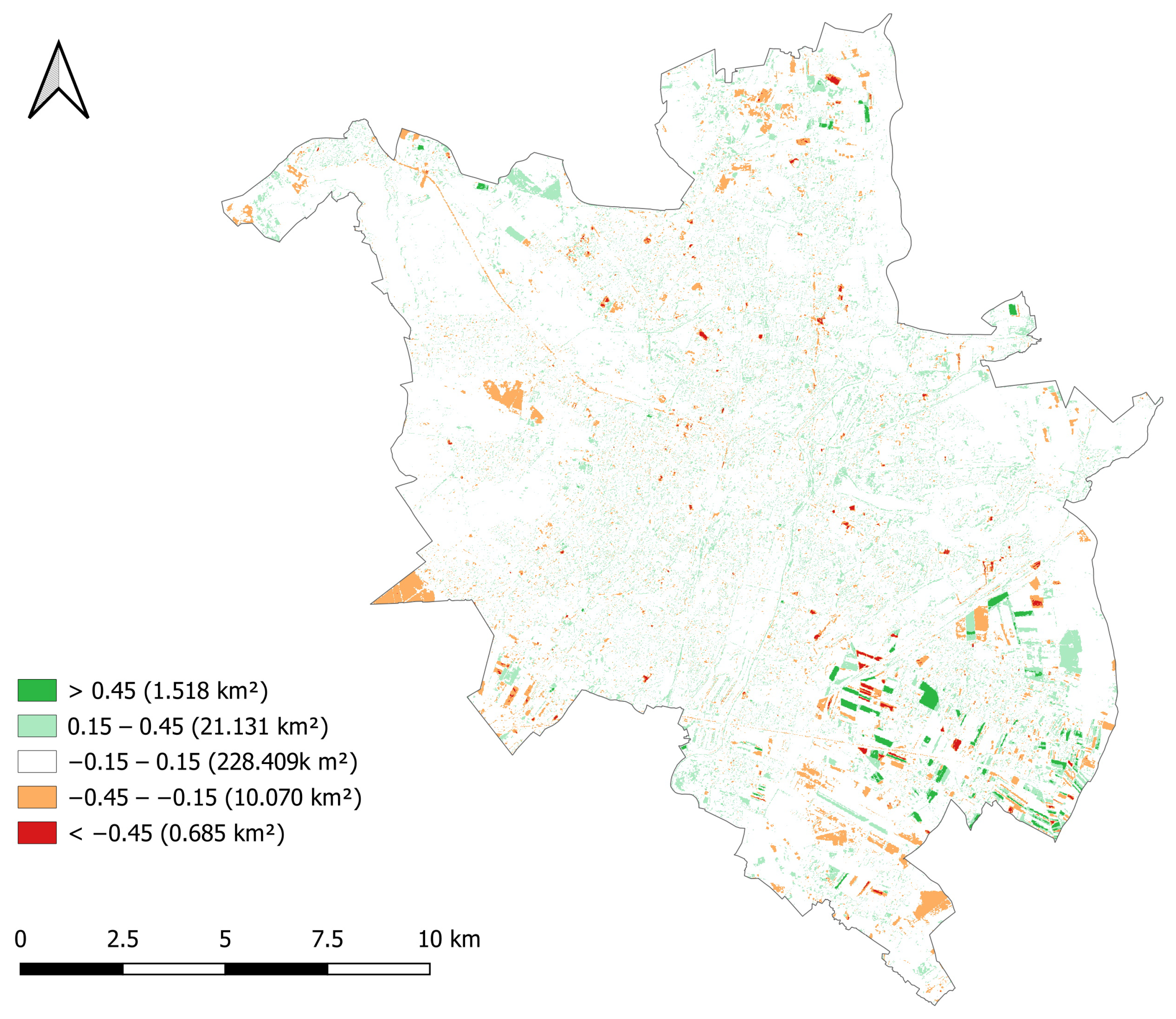
To identify areas within urban green spaces that experienced changes in size and tree growth during the analysed periods, the Normalised Difference Vegetation Index (NDVI) was used. The NDVI image is interpreted as an indicator of biomass. Its scale ranges from −1 to 1: elevated values are related to the photosynthetic activity of plants, together with the presence of chlorophyll that absorbs red light and parenchyma that reflects infrared light—the higher the index value, the greater the biomass at the location. Areas with negative values do not contain vegetation.

A comparison of NDVI changes was conducted on the basis of images taken over a two-year interval. The rasters were classified and subtracted using the Raster Calculator, creating new classes to indicate biomass gain (green) or loss (red) in specific regions. Figure 3 displays the resulting map. To correctly interpret this image, it was crucial to exclude areas dedicated to agriculture, which were considerably concentrated in the southern part of the city.

One of the main objectives of the SekoZ project was to create a 3D model of trees, as the main source of data for tree modelling was ALS (spatial characteristics: 12 p/m${}^2$, vertical accuracy 0.1 m, LAS, 2012). These data were compared with urban greenery information obtained from the City Inventory Database (CIB). Additionally, field GPS measurements and dendrological inventories were used in selected areas and Aquanet water protection zones. The reference layer was a DTM and the topographic database. Satellite imagery and orthoimagery were used to confirm tree canopy information produced by processing LiDAR data in the same area at certain time intervals. The 3D model incorporated nature conservation data acquired from the General Directorate of Environmental Protection, as well as 3D object models of buildings and a 3D tree layer in the openly accessible OGC standard cityGML 2.0.

2.2.2. Data Processing

To extract indicators of ecosystem service from previously collected information, an automated geospatial survey was carried out to map vegetation zones and identify areas with potential for designation as green spaces based on current development status, land ownership, and suitability for the maintenance and planning of UGS. Data were prepared to evaluate algorithms to estimate the removal of air pollutants (including CO${}_2$) in UGS, taking into account their characteristics, such as the leaf area index (LAI). A method of combining data from multiple sources was used, with the LiDAR data from ALS being the main one, to automatically determine the LAI index. Furthermore, an analysis of monthly fluctuations in LAI was performed using data sourced from the Copernicus Land Monitoring Service (CLMS). These data were acquired over a period of February to October. All spatial data were prepared in the Polish Geodetic Coordinate System 2000 (EPSG:2178) in a zone depending on the place of implementation. The elevation system of the data depends on the source data; this is usually the Kronstadt georeference system for Poland (PL-KRON86-NH) or, for the most recent data after 2019, Amsterdam layout (PL-EVRF2007-NH). This system is based on plane coordinates and altitude. DTM was used as a reference layer.

The system comprised several layers, which were created using the following steps to process the data:

• Source data layer (input for processing):
  • ALS data were used to generate tree models;
  • The tree models were compared with UGS data obtained from CIB and GPS measurements;
  • Tree models were incorporated into the DTM;
  • Satellite imagery and orthoimagery were used to collect information on tree cover in the same area at specific time intervals;
  • 3D building models in cityGML format and nature conservation data from the General Directorate of Environmental Protection (eliminating temporal information such as the crane in Figure 4) were used to create the 3D model;
  • BDOT10k data and a soil-agricultural map were used to calculate rainwater retention.
• Layer of data processed and objectified in the automation process.
  • The LiDAR point-cloud processing resulted in tree centroids, represented as points with their associated attributes;
  • Satellite image processing produced rasters through the classification and reclassification stages;
  • During the classification stage, the orthoimagery was converted into a raster representing the wooded areas;
  • Exposure and slope layers were obtained from the DTM.
• Analysis/calculation of a layer with developed/adapted calculation algorithms,
• An integration layer creation that allows for the aggregation and standardisation of the information presented in the system,
• A results layer generation for the presentation of data and results.

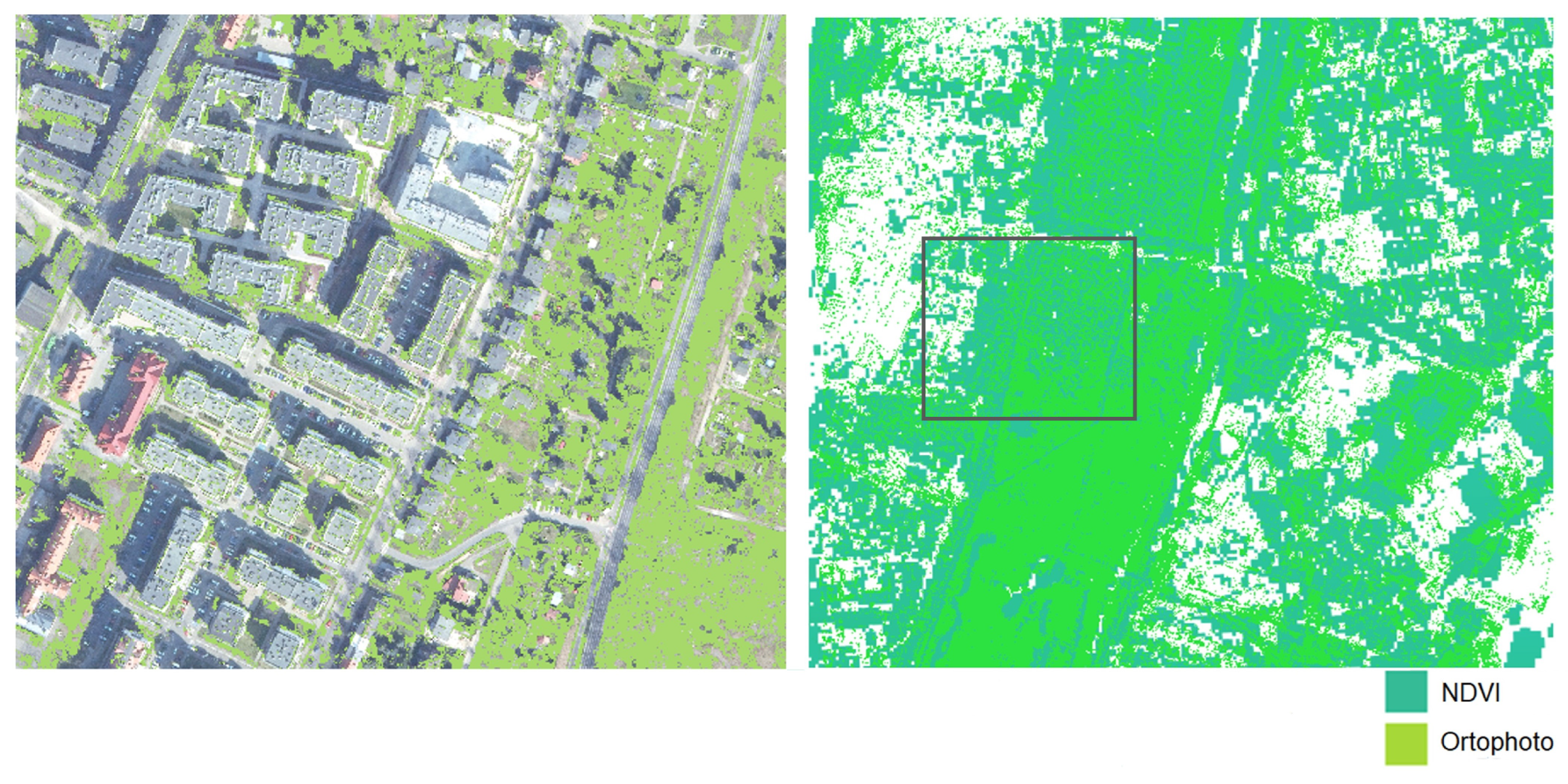
The transparent layer obtained from the orthophoto classification (see Figure 5, left) was superimposed on the layer obtained from the satellite images to allow for a comparison of the results (Figure 5, right side).

Following the processes performed on the LiDAR point cloud and data from the CIB, the output comprised layers of 3D tree models presented in the form of cylinders and symbols, along with files that contained tables (spreadsheets) linking the positions of the trees from one source to attributes from other sources. The spreadsheets summarise the tree displacement vectors obtained from the point-cloud detection, relative to the survey, and the coordinates stored in the CIB. The output also included reports on the calculation of the canopy volume, the reduction in CO${}_2$ and air pollutants, the effect of the green cover on the average temperature, and the intercept of precipitation. The results of the satellite and aerial imagery analyses were derived as raster files showing wooded areas and biomass growth from 2018 to 2020.

As a result of the analyses of the BDOT10k data using the soil-agricultural map and the DTM, a $50\times 50$ m basic field model was created, which included information on the vegetation and the building cover of the area in the database table. Layers also distinguished seven classes of rainwater permeability due to existing soils in the area, taking into account the variations in permeability in the soil profile [32,33]. The presentation engine processed the data and allowed for a 3 D (three-dimensional) presentation of the results. Web-based applications allowed the user to access the model and the results presented, and an application programming interface (API) layer allowed for the development and integration of the project.

2.3. Tree Detection—Quantitative Inventory of Urban Trees in Urban Space Based on 3D GIS Technology

Tree centroids obtained from aerial LiDAR data were used as the input for the process. The primary process for the simplification of the work was classification, where each point in the cloud was assigned with an attribute related to the object. An automatic filter was initially used to exclude points without the nearest neighbour (situated below the ground surface). Subsequently, the points located on the ground surface were selected. To differentiate high, medium, and low vegetation, three height intervals were introduced relative to the approximate surface of the ground. The precision of the ground classification significantly impacted the quality of the vegetation data. The building selection algorithm relied on the single echo produced by reflected laser beams, in contrast with vegetation, which produces several consecutive echoes.

Classification was automated; however, manual editing of individual points was usually required if they were outside the limits of the correct area as a result of the algorithms [34]. The classification process in this case comprised the following steps:

• Exclusion of non-nearest neighbour (random) points—automatic filtering;
• Selection of points on the ground—random pairs of adjacent points were tested for distance and tilt angle;
• Extraction of buildings that produce an echo from vegetation that produces multiple consecutive echoes and
• Classification of vegetation based on specified height ranges: low (0.0 m to 0.4 m), medium (0.4 m to 2.0 m), and tall (2.0 m and above).

The medium and high green classes were extracted to generate the data. Subsequently, a search algorithm was used to locate the points that make up a single tree. The position of the tree trunk was estimated by finding the centroid of the crown contour, which was recorded by LiDAR and represented in vector format by points. Clustering was executed, after which each tree was assigned an ID. This consolidated all relevant data obtained from the scanned crown and its vector representation. When there was uncertainty about the position of the crown contour centroids, semi-automated centroid determination was used. In cases where uncertainty still persisted, a GPS measurement was taken in the field to determine that point.

Data were presented in vector format as points representing the estimated position in the field of a tree trunk whose crown was identified by LiDAR. The selected classification method was the maximum probability approach, which calculated the probability that each pixel belongs to a particular class and assigns it to those with the highest probability. For each class, a mean and variance–covariance matrix was computed to categorise the pixel. The result of this process generated a layer comprising individual tree centroids, each with their corresponding attributes. Each entity included the X, Y, and Z coordinates of the centre of the tree mapped on the DTM. Additionally, the attribute table included the ID. This process facilitated the calculation of the diameter, area, or volume of the tree by combining points into voxels using 3D geometry. The point’s coordinate determined the hypothetical location of an individual tree’s trunk. Tree centroids were identified, resulting in cylindrical representations of trees that provided both visual and descriptive information on the hypothetical trunk position, height, and crown span. The Scaler tool was used to adjust the diameter of the tree and to create varying tree sizes in cylindrical models.

2.4. Procedure for Tree Trunk Analysis in Basic Fields

The developed procedure consisted of several functions that analysed different aspects of the tree trunks in the network. In each analysis, an SHP 2D file served as the basis, containing identified tree trunks from a point cloud and descriptive attributes for statistical analyses. The analysis of the data was carried out for the network and derived the following parameters:

• Mean height of the trunk in the network.
• Minimum height of the trunk in the network.
• Maximum height.
• Number of trees in the plots.
• Mean height weighted by crown area.
• Area of crown projection on the ground plane.
• Percentage area of crown projection on the ground plane in relation to the total mesh area: The statistical data file for the network were loaded into FME using the SHP reader and analysed in several parallel paths to produce results based on different indicators. Geometries were generated in the form of 3D solids whose height depended on the parameter being analysed, and that took into account the visualisation component.
• Number of trees—the algorithm defined the height of the visualisation/solid as 150 m + the number of trees in the grid.
• Weighted height—tree height is defined as 150 m plus 10 * weighted height in the grid.

2.5. Urban Greenery Data Objectification

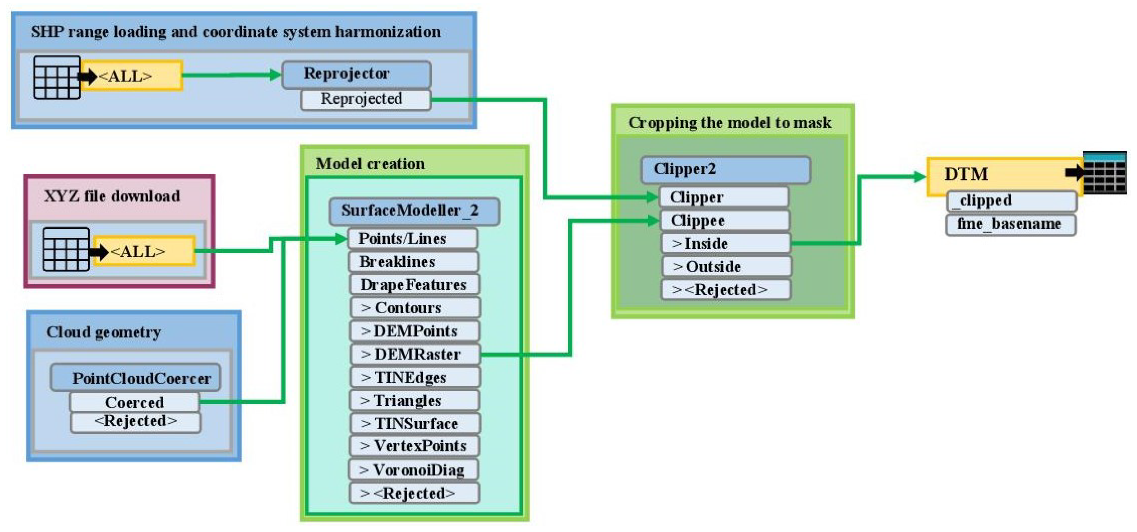
A multistep processing algorithm was developed for the project, as depicted in Figure 6.

• DTM was created in the ASC format (Figure 6).
• Datasets loaded: two shapefiles with the tree location points were loaded (one set was the CIB—point data and the other was the LiDAR point cloud—polygon data).
• Assignment of the Z coordinates: Hypothetical tree trunk location data from the LiDAR point cloud were assigned X, Y, Z coordinates to each point. The data set representing the trees inventoried extracted from the CIB did not possess elevation coordinate information, so the X, Y data were projected onto the surface of the DTM and the points were assigned a coordinate before proceeding to the next step of reading the Z coordinates.
• Removal of geometries: In the next step, the geometry of the objects was removed in parallel for both sets, replaced by a template (proportional to the diameter of the tree), and the symbols were provided a third dimension.
• Assignment of attributes.
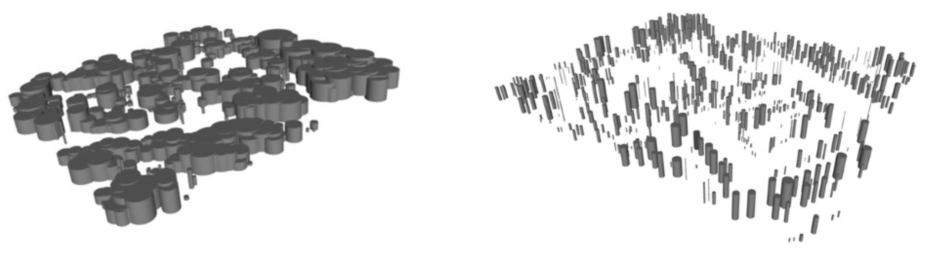
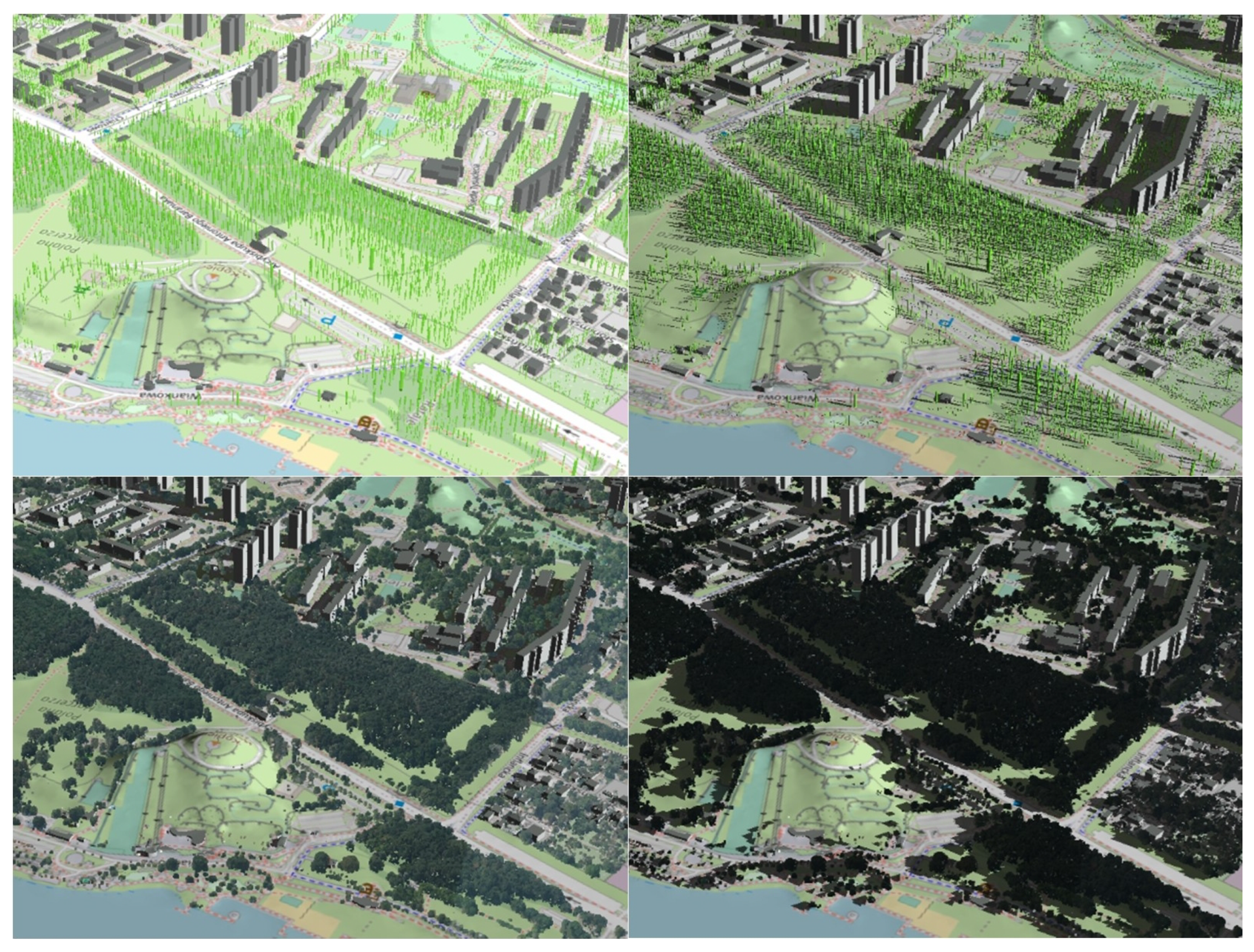
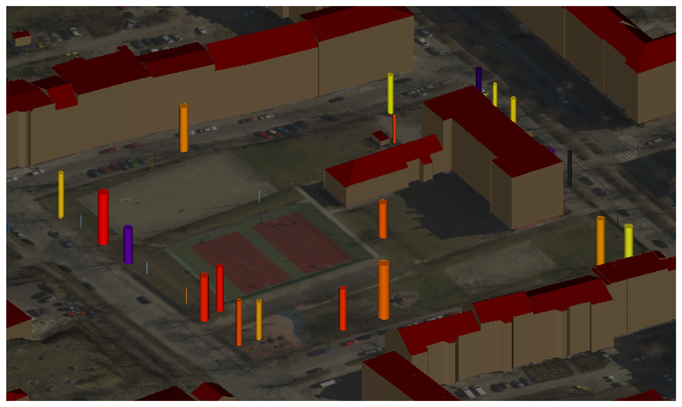
• Merging the two datasets, recording the results, and generating statistics. The result was a tree model in the form of cylinders. This model was easier to analyse (Figure 7—left).
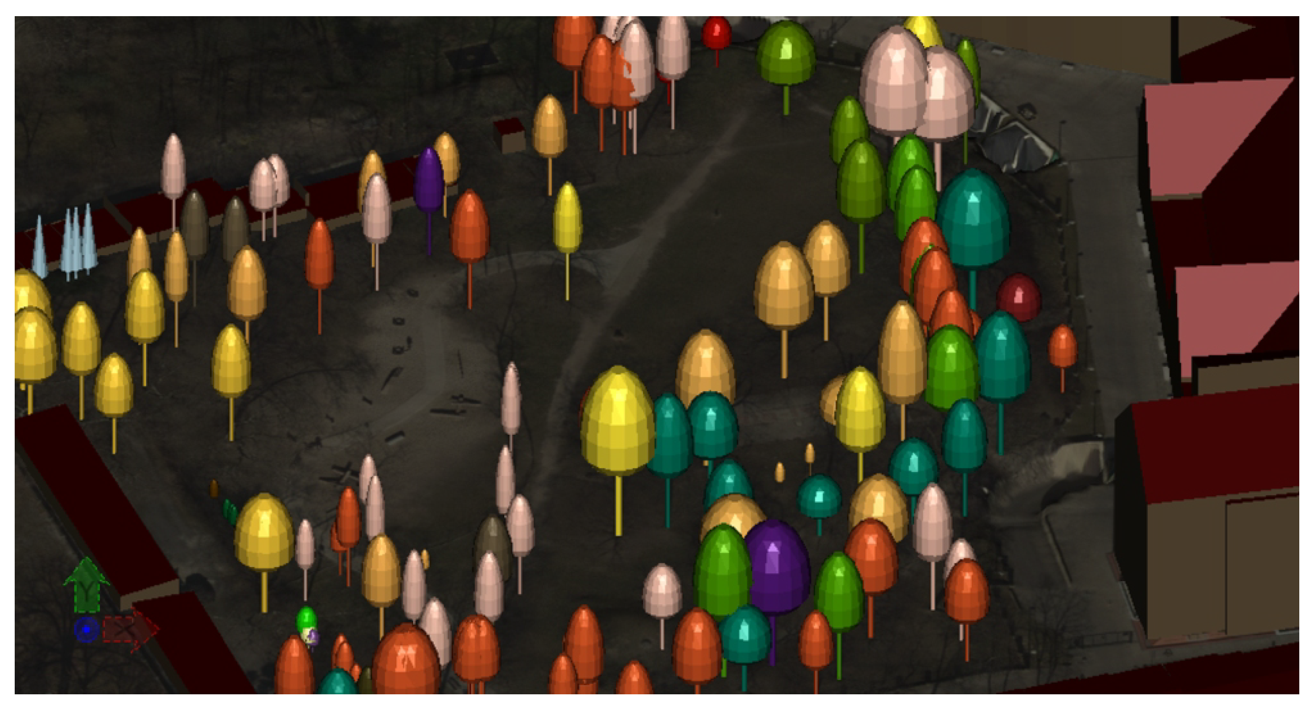
• Creation of a more aesthetically pleasing model for visualisation. This was achieved by replacing the geometry of the objects with ready-made 3D models of trees, thus distinguishing between deciduous and coniferous trees.
• Duplicate control: Because of the differences in the number of input and output objects, a duplicate ID check was also performed on the database independently using the CIB.

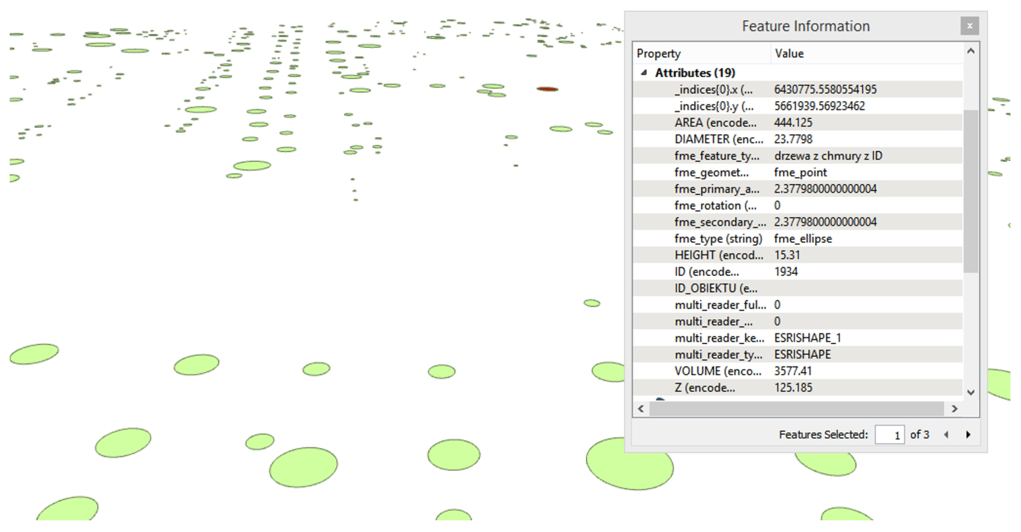
The process of creating 3D tree models in the form of analytical columns and vector models, combining attributes from both databases, and recording the results and statistics obtained began with the objectification of the urban greenery data. Observing the results of the different steps of the algorithm, it was found that a new geometry was input in the form of circular polygons, but it was not defined in terms of size and it was not linked to the object coordinates (default coordinates at the beginning of the coordinate system). Therefore, the next step was to determine the size of the circle depending on the size of the tree that it was supposed to represent. A dependency on the actual value of the tree diameter was defined (the radius was assimilated to half the value of the DIAMETER attribute). This resulted in circles of different sizes.

The geometry was then moved from the origin of the coordinate system to specific locations representing the X, Y, Z coordinates of each tree. When generating the 3D geometry of the trees, a vertical direction was selected in the extrude parameters, and the value depended on the values of the HEIGHT attribute (Figure 7—left).

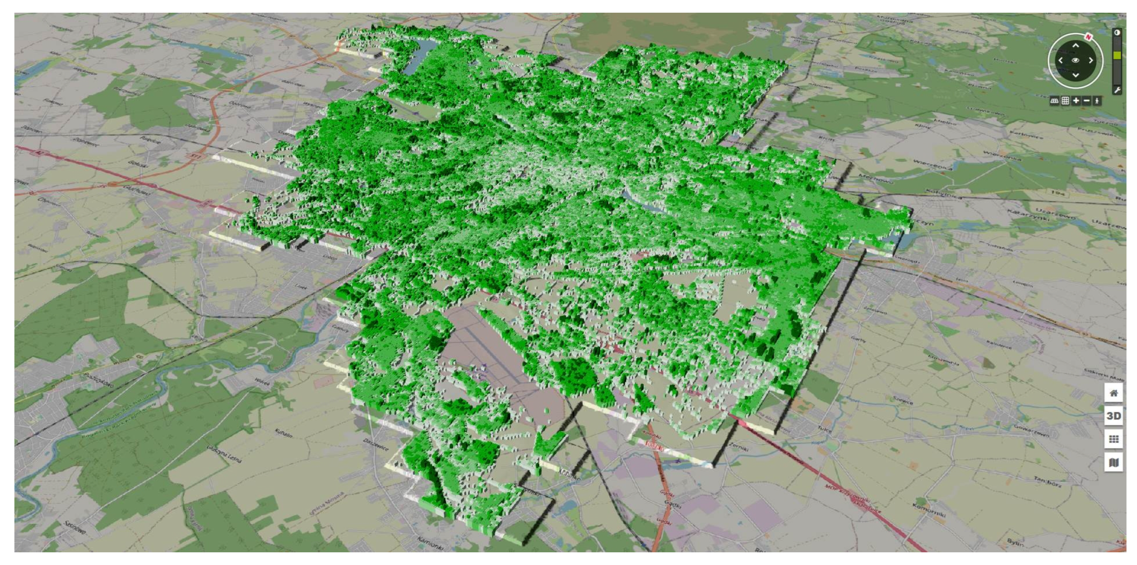
However, the resulting models were visually unacceptable. Solids representing individual objects blend together and result in a difficult interpretation. This type of urban greenery representation could be applied to the analysis of air corridors, where the actual extent of the tree canopy is important. However, in this case and for visualisation purposes, an additional parameter was introduced by defining the scale after X and Y as 20% of the tree diameter value (Figure 7—right and Figure 8).

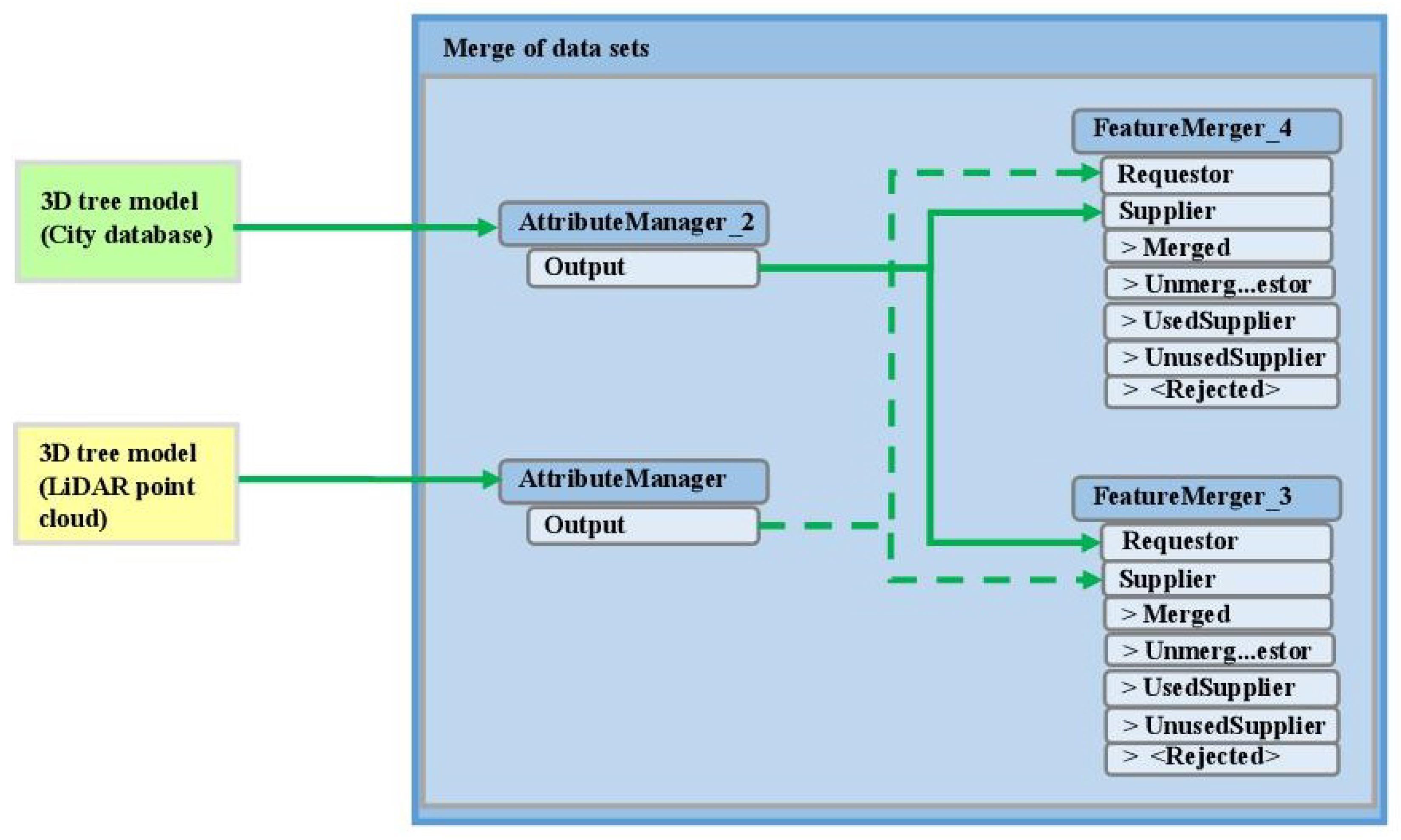
2.6. Verification of 3D Tree Models

The crown cover of the tree was also estimated. The use of symbolic models to represent 3D trees was demonstrated using CIB as an example. A geometry merge effect was added as an input file for the next step. To be able to combine two data sets from different sources, common identifiers had to be established. For this purpose, the CIB tree identifiers were considered to be the most appropriate. Therefore, this part of the task started by mapping the identifiers. Before assigning attributes, their names were edited by adding the prefix ’D’ to each column in the table of trees resulting from the point-cloud detection. This task was achieved with the purpose of making recognisable features from different sources easier. The attribute manager function was used to do this (Figure 9). This transformation was also used in the second data set to introduce clearer coordinate labels.

As a first step, the 3D tree models were verified against data from the tree inventory database. First, the positional differences of the trees generated from the point cloud were investigated against the data obtained from CIB. A four-stage semi-automatic verification process was carried out, consisting of the following steps:

• Comparison between two databases. Object data acquired through LIDAR were identified in the CIB and compared with their centroids.
• Any objects present in both databases were marked as certain. Such objects were provided combined information from both sources.
• Verification involved extracting the trees that were not found in the CIB from LiDAR. Objects were only added to the database if their presence was confirmed by an orthophoto or topographic map.
• Trees not present in the LiDAR were extracted from CIB and surveyed as in the previous point.

Additional verification was carried out using drones and field surveys in two areas where the presence of trees from the LiDAR data and CIB was unclear. From the results presented, it can be observed that most of the generated objects were characterised by a displacement vector not exceeding 0.5 m, and only a small proportion exceeded 1 m. This may be due to the specific arrangement of the tree crowns. For example, CIB showed that there was a 16 m tall small-leaved lime tree with a “V”-type branch and a 30° slope, which, with a crown diameter of 12 m, could have complicated the accurate estimation of the position of the hypothetical trunk from the point cloud.

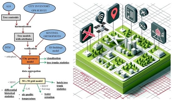
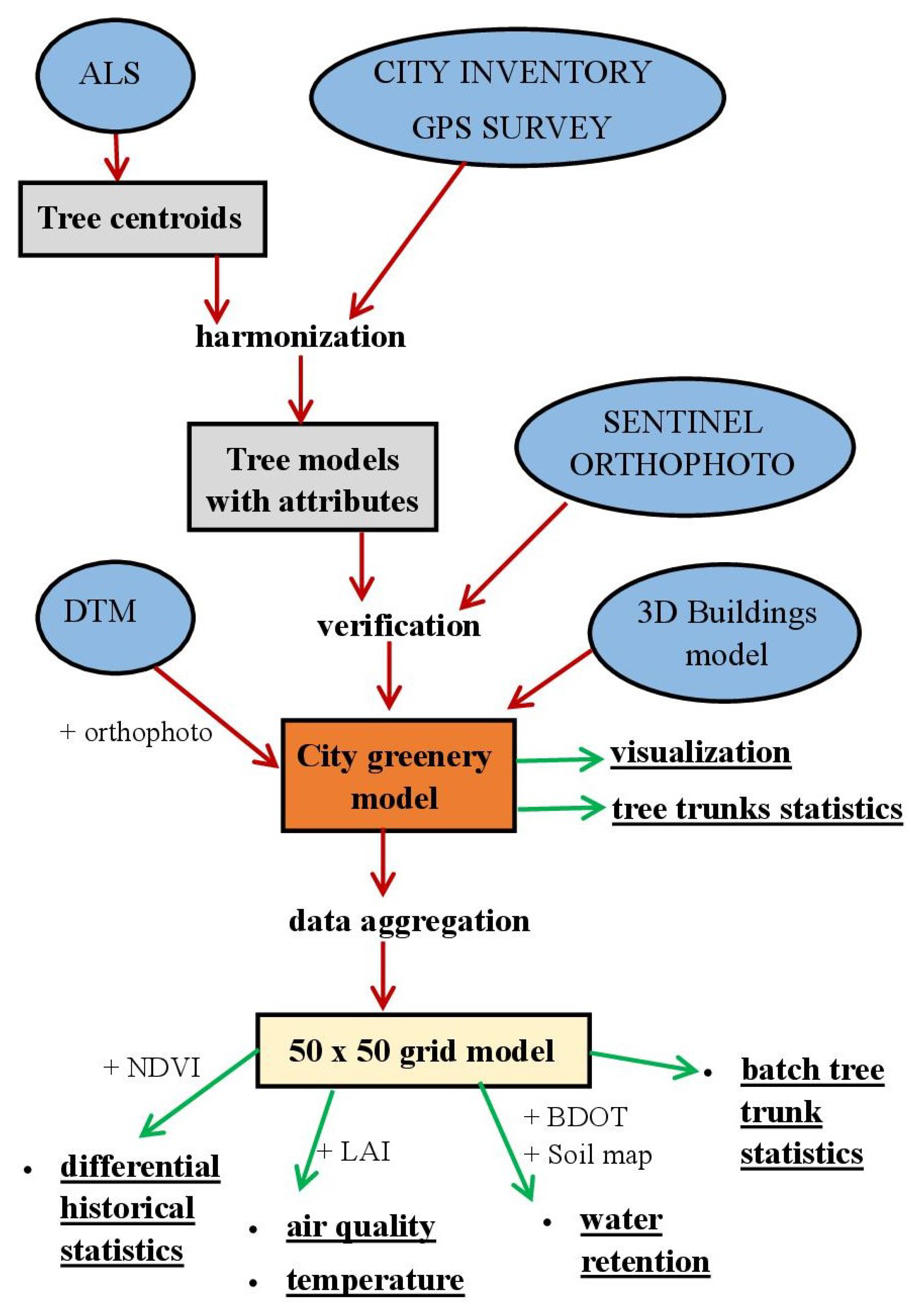
A general scheme showing the project workflow is depicted in Figure 10. This figure shows the general data sources, algorithms, and outcomes of the SekoZ project.

Geoportal SekoZ

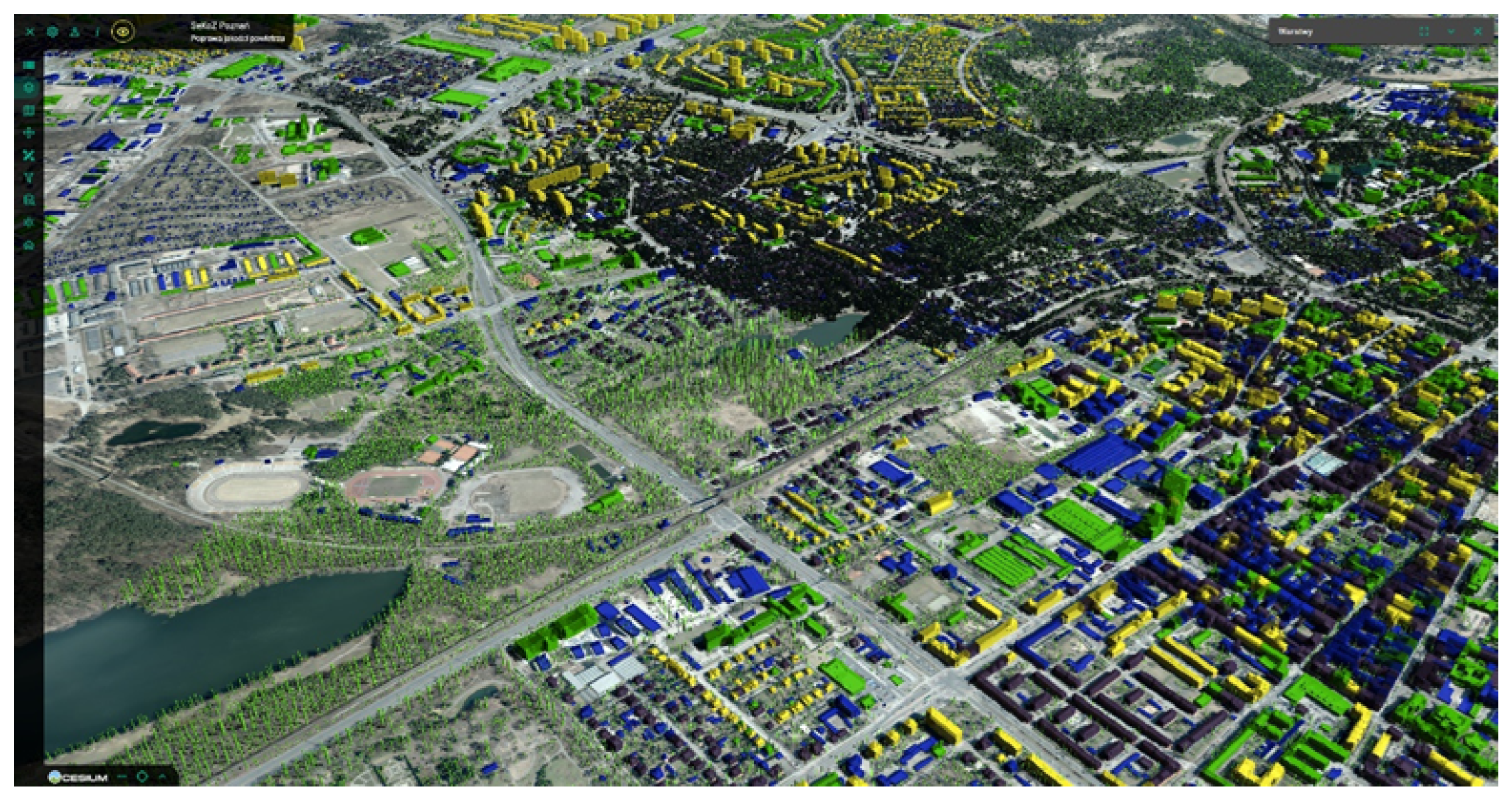
An integral part of the SekoZ project is an IT tool, the Geoportal for Spatial Information of the company SHH with its own name and objectives (see Figure 11): Geoportal SekoZ. The application uses Cesium Virtual Globe technology. Depending on the configuration in the administrator panel, it contains an integrated set of tools for presenting, viewing, and analysing the spatial data of the 3D city model.

Geoportal SekoZ as a Spatial Information System, is a web-based application that presents 2D data and 3D models, integrating spatial with descriptive data. The information and functional content depend on the user’s needs, which are defined by the administrator according to their role in the system. The data presented in the system come from many different sources. They are collected during the implementation phase and can then be updated as required to publish a base model for end users. This may include data such as landform and land use, geological structure and soil profile, greenery records, address point records, development model, and other elements of the urban infrastructure.

The SekoZ Geoportal is an application aimed at the authority’s internal users. It enables assigned users with editorial rights to define active scenarios for compact urban green areas. These scenarios can be viewed, printed, or analysed by users who can only access the data. The tool combines viewing capabilities for both vector and raster spatial data, as well as the ability to search and analyse vector data based on its descriptive attributes and geometry. Furthermore, the administrator panel facilitates the generation of system data compositions and their expansion.

SekoZ Geoportal is compatible with any computer or workstation equipped with a web browser that supports JavaScript and WebGL scripting (the JavaScript language API used for rendering 3D computer graphics in a web browser devoid of further plug-ins). The software has been developed using responsive technologies, which facilitates its successful use on mobile devices. However, the acquisition of significant 3D data from the mobile web may affect its performance.

3. Results

3.1. Model of Urban Greenery

The result of the algorithms applied is tree models in the form of columns that contain visual information on the estimated position of their hypothetical trunk, height, and one fifth of the diameter of the crown, as shown in Figure 12, Figure 13 and Figure 14. A general overview of the results is also shown in the lower part of Figure 10.

Figure 12 illustrates the output of the applied methodology on a medium scale, where thousands of trees were already analysed for an area with extensive green spaces. In addition, areas without trees were identified and visually mapped correctly using the SekoZ geoportal application.

Figure 13 shows another example of the three-dimensional visualisation of the city of Poznań using the SekoZ geoportal. In this figure, the integration of the 3D tree model combined with the information obtained from other data bases, such as the height of the buildings in a more urbanised area, is depicted. However, the results of the workflow are better appreciated in Figure 12.

The combination of the two data sets opens up the possibility of performing various analyses using arithmetical functions, such as calculating volumes, height differences (Figure 15), or tree position vectors, which have been incorporated into the overall algorithm of the project.

Additional analyses, such as the shading analysis, depicted in Figure 14, can also be performed using the information stored during the construction of the 3D tree model.

3.2. Presentation of the Model According to the Purpose of the Stand and the Tree Species

A more visually appealing layer in the form of symbolic 3D tree models was used to present the tree model on its own. The colours (symbology) of the individual objects were set according to the purpose attribute. The model was also visualised by tree species (Figure 16). This visualisation shows that the area under study contained mainly acacias (yellow), linden trees (green), horse chestnuts (light brown), and maples (light green). A colour analysis carried out on the three-dimensional tree models is an interesting approach to facilitate the management of urban greenery. If the area were extended to the limits of the entire city, many new applications and statistics would be possible.

3.3. Data Aggregation

Processing a large number of data sets across an entire urban area, 262 km${}^2$ for the city of Poznań, required an optimised approach for the different stages of project preparation. The choice of computational parameters not only affected the accuracy and computation time of the resulting ecosystem service parameters, but also had a significant impact on the quality of the system user’s interaction with the 3D model. The first element of the system performance to be optimised was the choice of the size of the computational grid. System selection and performance tests were carried out on different sized meshes, i.e.,: $200\times 200$ m/$100\times 100$ m/$50\times 50$ m/$25\times 25$ m.

The selection of meshes with the mesh sizes given for testing was determined by three aspects:

• Analysis of the availability and resolution of the batch sets for the calculation procedures;
• The selection of multiple computational runs for the resulting parameters of individual ecosystem services requiring a consistent computational grid for all runs;
• The overall performance of the system and the time required for the calculations.

The discrete computational grid ($50\times 50$ m) aggregated any number of objects into discrete fields, which provided a discrete model for computation, and balanced the value and precision of the data (Figure 17).

The data obtained from the CIB and remote sensing were preserved in the model, which enabled batch statistics to be used for the estimation of other tree parameters:

• Average tree height—average of the pixels considered as a tree (Figure 18—below),
• Percentage of canopy cover—average of the pixels considered as a tree related to the remaining area,
• Leaf index,
• Descriptive information—from the CIB.

By modelling urban space objects in this way, it was possible to provide input for high-resolution calculations of urban green ecosystem services. The basic object values imported into the grid were, in particular:

• Number of buildings,
• Average height of buildings,
• Number of trees (Figure 18—above),
• Average height of trees,
• Minimum tree height,
• Maximum tree height, and
• Percentage mesh coverage of the tree crowns.

Reducing the vector fields presented in the 3D model to discrete values in the grid was essential for developing input for high-resolution modelling.

3.4. Simulation of the Impact of Planned Developments and Tree Cover on Urban Air Quality

Estimation of the impact of urban greenery on air quality, rainwater retention, and mean temperature in the city was estimated based on tree data from the point cloud detection of aerial scans for the city (e.g., carbon dioxide uptake is depicted in Figure 19)—the models and formulas used for this analysis are described in detail in [33].

Emissions during the winter seasons are higher; however, as there are no leaves on the trees, the obtained figures can be very similar, and this can lead to an error in the interpretation of the results. Therefore, Figure 19 depicts the carbon dioxide uptake for the months in which the emissions were noticeable using the algorithms applied.

The approach presented in this contribution assumes that the benefits of trees depend on the size of the crown projection area and the LAI (Figure 20). The trees were divided into three groups: small, medium, and large. In case of ambiguity when selecting a class for the trees, the crown diameter criterion was considered the most important. Both the parameters applied to divide the trees into groups and the averages used in the calculations were adopted from a study conducted in Warsaw [35].

4. Discussion

One of the most challenging aspects regarding the modelling of the model presented and the subsequent calculations was the integration of multiple data sources, many of which were incomplete and contained duplicates and/or data inconsistencies. Therefore, each data source had to be verified for accuracy and completeness and then verified after data integration. The authors proposed different algorithms to decrease the uncertainty in the results derived from the tree model and, consequently, in the results of the further analyses. However, the model presented also provided useful results when applying the concept of smart city taking into account the importance of greenery and the presence of tress within urban areas.

The comparison between the extent of the greenery according to the NDVI index and the extent vectorised from orthoimagery demonstrated that the data differed mainly in the level of detail. The wooded areas extracted from satellite imagery (NDVI) covered larger parts of the city than those obtained from aerial photo classification. On the one hand, aerial photography classification allows foreasy and fast extraction of land cover information, its polygonisation, and their use in the presented analyses. On the other hand, processing satellite images helps to monitor the condition of forests and to track changes in urban greenery. On the basis of this type of raster data, it is possible to calculate the total biomass growth in an urban area over a given time interval.

Three-dimensional models of individual trees derived from ALS possess the advantage of allowing individual analyses, where phenomena do not have to be examined on an area basis, but can be analysed in terms of tree spacing, as well as differences in height, volume, or diameter. Furthermore, NDVI is sensitive to vegetation types, amounts, and spatial scales [36]. However, its use in urban areas should be carefully evaluated. Data extracted from satellite imagery can be used to analyse the distribution of greenery within the city. By calculating the NDVI index, biomass growth can be monitored, the condition of green areas can be studied, and appropriate measures can be planned for the sound management of the green infrastructure. However, the data are not detailed and can only be used for the analysis of larger areas. While the NDVI index provides information on tree condition and chlorophyll content, LiDAR cloud models of trees provide information on the physical dimensions of each tree. However, trunk generation is based on crown segmentation, so groups of trees whose branches are close to each other possess a limitation.

In addition, trees less than 2 m tall can represent another problem. These trees are not classified as tall greenery in the hypothetical stem-generation process, and have low-lying crowns that are obscured by the crowns of taller trees [37]. Here, the only source of information is the CIB. Inaccuracies can also be caused by trees that have fallen since the LiDAR survey and are already included in the CIB. The trunks of these fallen trees are often very close to others, so their presence may have compacted the point cloud and contaminated the data, overstating the diameter or shifting the point of a hypothetical trunk.

5. Summary and Conclusions

The methodology presented in this paper allows for efficient and reliable data integration, making full use of the availability and diversity of data sources. The final result of the algorithms and procedures was an innovative and new tool to support decision-making processes and allow for the integration of urban greenery data into smart city management. The functionality of the developed tool was based on the following components:

• A source data layer (input for processing);
• Processed/objectified data layer in the automation processes;
• An analysis/calculation layer;
• An integration layer allowing fpr the aggregation and standardisation of the information presented in the system;
• Output layers (CityGML) containing elements for the presentation of the data and results.

As a result of the processes performed using the LiDAR point cloud and the data from CIB, the final output was the generation of layers of 3D tree models in the form of cylinders and symbols, as well as files containing tables linking tree positions from one source with attributes to other complementary sources. The results of the data analysis were stored in spreadsheets (databases) containing a summary of the tree displacement vectors from point cloud detection relative to the survey and the coordinates stored in the CIB. The results also included reports on the estimation of canopy volume, CO${}_2$ reduction, and pollutants in the environment; the effect of greenery on average temperature; and the intercept and absorption of precipitation.

The results of the satellite and aerial imagery analyses were derived from raster images showing forest cover and biomass growth from 2018 to 2020. As a result of the work on the BDOT10k data using the Global Agricultural Map and the DTM, a $50\times 50$ m basic field model was created. This model contained information on the coverage of a given area by the five rainwater permeability groups in a DBF table, as well as an example of the calculation of the retention factor (and other ecosystem services) in raster form, as follows:

• A database layer that stores the system’s data and results;
• The engine for presenting data and results in a three-dimensional view;
• Web applications for user access to the model;
• An application programming interface (API) layer, which allows for the development and integration of the SekoZ system with other data sources and systems.

The architectural concept of the SekoZ project includes the creation of an output layer consisting of an application environment and a set of tools to manage data sets, process them into a usable form, and configure sets of 3D models.

As mentioned above, one of the key features of the applied algorithms is the process for converting input data into data structures for efficient visualisation in a web browser. The following data conversion processes are supported: conversion of the terrain model (DTM) to a mesh format (Quantised Mesh) for displaying the optimised terrain model in the CesiumJS virtual globe environment: (i) conversion of 3D data to 3DTiles format for display in CesiumJS and (ii) conversion of raster data (aerial photographs, cadastral maps, base maps, topographic maps, etc.) into the Tile Map Service (TMS) structure.

In addition to the data sources presented, the possibility of linking already existing web services as terrain overlay is assumed. The system supports the following services: (i) TMS, i.e., services conforming to the Tile Map Service specification, and (ii) WMS services, i.e., services conforming to the OGC Web Map specification (1.0, 1.1).