Article

Spatiotemporal Analysis of Soil Moisture Variability and Its Driving Factor

1
College of Resources and Environment, University of Chinese Academy of Sciences, Beijing 100049, China
2
Yanshan Earth Critical Zone and Surface Fluxes Research Station, University of Chinese Academy of Sciences, Beijing 101408, China
3
Faculty of Land Resources Engineering, Kunming University of Science and Technology, Kunming 650093, China
4
Key Laboratory of Agricultural Remote Sensing, Ministry of Agriculture and Rural Affairs, Institute of Agricultural Resources and Regional Planning, Chinese Academy of Agricultural Sciences, Beijing 100081, China
*
Author to whom correspondence should be addressed.
Remote Sens. 2023, 15(24), 5768; https://doi.org/10.3390/rs15245768
Submission received: 28 October 2023 / Revised: 12 December 2023 / Accepted: 15 December 2023 / Published: 17 December 2023
(This article belongs to the Section Remote Sensing in Geology, Geomorphology and Hydrology)

Abstract

:
Soil moisture (SM), as a crucial input variable of land surface processes, plays a pivotal role in the global hydrological cycle. The aim of this paper is to examine the spatiotemporal variability in SM in the Heihe River Basin using all-weather land surface temperature (LST) and reanalysis land surface data. Initially, we downscaled and generated daily 1 km all-weather SM data (2020) for the Heihe River Basin. Subsequently, we investigated the spatial and temporal patterns of SM using geostatistical and time stability methods. The driving forces of the monthly SM were studied using the optimal parameter-based geographical detector (OPGD) model. The results indicate that the monthly mean values of the downscaled SM data range from 0.115 to 0.146, with a consistently lower SM content and suitable temporal stability throughout the year. Geostatistical analysis revealed that months with a higher SM level exhibit larger random errors and higher variability. Driving analysis based on the factor detector demonstrated that in months with a lower SM level, the q values of each driving factor are relatively small, and the primary driving factors are land cover and elevation. Conversely, in months with a higher SM level, the q values for each driving factor are larger, and the primary driving factors are the normalized difference vegetation index and LST. Furthermore, interaction detector analysis suggested that the spatiotemporal variation in SM is not influenced by a single driving factor but is the result of the interaction among multiple driving factors, with most interactions enhancing the combined effect of two factors.

1. Introduction

Soil moisture, as a critical parameter characterizing global land surface hydrological cycles, has extensive applications in various fields, such as hydrology [1,2], meteorology [3,4], climatology [5,6], and water resource management [7,8]. It serves as a crucial state variable in the climate system, governing the exchange of water, energy, and carbon fluxes between the land surface and the atmosphere. SM is one of the key input parameters in land surface processes and global hydrological cycles. However, due to the significant spatiotemporal variability in SM across different dimensions, the study of this variability is very important when exploring the spatiotemporal distribution of SM and its additional applications [9].
Numerous scholars have extensively investigated the spatiotemporal variability in SM and proposed various research approaches based on this foundation. Initially, researchers mainly used traditional statistical methods, such as the probability distribution [10], standard deviation [11], and coefficient of variation [12], to study SM variability. However, geostatistical methods, which entail the incorporation of spatial information and focus on the spatiotemporal distribution of samples, have been verified as more effective than traditional statistical methods in studying SM variability in time series or spatial contexts [2,13]. As the wavelet analysis methods gained prominence in investigating the temporal distribution of surface parameters, researchers have provided a novel approach for analyzing the spatiotemporal variability in SM. Wavelet transformation primarily aims to decompose time series into the time–frequency domain, thereby revealing significant fluctuation patterns of time series, including cyclic variations, and the temporal patterns of these cyclic variations [14]. Numerous scholars have focused on this area as well. For instance, Das and Mohanty [15] utilized the Haar wavelet multiresolution analysis based on SMEX02 data to investigate spatial differences in SM variations. Lee and Kim [16] explored wavelet coherence between ecological–hydrological meteorological factors and SM in the Sulmachun watershed. Furthermore, methods such as empirical orthogonal functions (EOFs) [17] and rotated principal component analysis (RPCA) [18] have demonstrated significant advantages in studying SM variability.
In recent years, given the significant advantages of spatial stratified heterogeneity (SSH) in quantifying the stratified regularity of physical surface parameters, it has been widely applied in the study of SM. SSH refers to the phenomenon whereby the variance within a layer of surface parameters is lower than that between layers, representing the stratified regularity manifested in spatial heterogeneity [19], which can be specific to classification or zoning. Based on the q-statistics method, Wang et al. [20] first proposed an important method for studying geographical spatial differentiation—the geographical detector (GD) model. Subsequently, numerous scholars have employed this model to investigate spatial heterogeneity and changes in the driving factors of surface SM. For example, Yang et al. [21], Xu et al. [22], and Yang et al. [23] used the GD model to assess the spatiotemporal patterns of SM on the Inner Mongolian Plateau, the Ili River Basin, and the Shiyang River Basin, respectively, offering a novel research perspective for the analysis of the spatiotemporal patterns of SM. Due to the sensitivity of the GD model relative to spatial discretization methods and the number of strata, determining both can be relatively complex. To address this challenge, Song et al. [24] built the GD model and developed the OPGD model, which aims to achieve the best combination of spatial data discretization methods and the number of strata. This enhancement has made subsequent GD models more accurate, flexible, and stable [24], significantly improving the practicality of the GD model. Zhang et al. [25] proposed a robust geographical detector (RGD) model to overcome the sensitivity limitations of spatial data discretization and provide a robust and reliable solution for exploring spatial correlations and identifying geographical factors. Additionally, Luo et al. [26] developed a geographical optimal zone heterogeneity (GOZH) model capable of finely partitioning subregions and applied it to study the determinants of the spatiotemporal differences in SM in the Northern Hemisphere, yielding promising outcomes.
Additionally, Vachaud et al. [27] observed that when examining the approximate spatial order of SM at different times, there is a certain probability that the order of the SM content at different sites will remain constant over time. This suggests that SM displays temporal stability. In contrast to the spatiotemporal variability in SM, the temporal stability of SM emphasizes the unique temporal patterns of SM variation. It holds considerable importance in revealing time series changes in SM information and the influence of SM on the surface–atmosphere exchange of matter and energy.
Previous studies revealed that SM is the result of various driving factors, including soil texture and structure [28,29,30], topographic features [31,32,33], land cover patterns [34,35,36], and meteorological forcing [37,38,39]. These factors exhibit nonuniform distributions in both time and space, giving rise to the unique spatiotemporal distribution patterns of SM. However, the degree to which each driving factor influences SM varies at different scales [40]. Soil physical properties, such as field capacity and soil texture, affect SM distributions by influencing soil hydraulic properties, and this characteristic is more pronounced at field scales. For instance, Crave and Gascuel-Odoux [28] found that at the 1 km scale, the dominant factors influencing SM spatial heterogeneity are terrain factors and soil physical properties. At the watershed scale, terrain features play a more significant role in determining the SM distribution. Charpentier and Groffman [31] observed that the complexity of the terrain contributes to an increase in SM spatial heterogeneity, and Moore et al. [32] studied the relationship between terrain attributes and the surface SM distribution in an agricultural watershed, revealing that terrain nonuniformity is a primary factor controlling the SM spatial variability at the watershed scale. Land cover patterns exert a greater impact on SM at the watershed, especially at regional scales than other factors. Wang et al. [34] investigated the influence of vegetation on the SM spatial distribution and found that during the growing season, vegetation exerted a stronger impact on the SM spatial heterogeneity than that during the nongrowing season. Meteorological factors, such as precipitation, temperature, and climate type, play a more significant role in SM variabilities at the regional and even continental scales compared to other variables. According to Liu et al. [37], precipitation events significantly impact the SM response in the desert area of Heihe River Basin. In arid regions of China, precipitation positively affects SM, while temperature yields a negative impact, with precipitation contributing more notably to SM changes than temperature [41]. Crow et al. [40] found that the soil texture and structure, topographic features, land cover patterns, and meteorological forcing all impact SM across all scales, but their impacts vary in degree across different scales. Therefore, when analyzing the spatiotemporal patterns of SM or conducting driving force studies, it is crucial to carefully consider the combined effect of these driving factors on SM.
This study, based on downscaled SM data, utilized classic geostatistical methods—the semivariogram function and standard deviation analysis—to examine the spatiotemporal distribution patterns of SM. Via the semivariogram function, we gained insights into the geographical variations of SM, unveiling differences and correlations among different locations, thereby providing robust support for the further exploration of SM’s spatiotemporal distribution. Meanwhile, the standard deviation method allowed us to quantify the internal dispersion of the SM dataset, offering a more comprehensive understanding of the fluctuation characteristics of the SM time series. Furthermore, in analyzing SM in the Heihe River Basin, this study employed the OPGD model, which carries unique advantages and necessities. By optimizing spatial data discretization methods and stratification strategies, this model could more accurately delineate the study area and identify SM characteristics within distinct spatial zones. This model can provide a more precise revelation about the spatiotemporal drivers of SM, aiding in comprehending the factors and mechanisms governing the monthly distribution of SM in the Heihe River Basin.
The objective of this study, using the aforementioned methods, was to uncover the spatiotemporal distribution patterns and driving forces of SM in the Heihe River Basin, aiming to provide scientific foundations and technical support for water resource management and ecological conservation in this region.

2. Materials and Methods

2.1. Study Area

In this study, we primarily adopted the Heihe River Basin as the research area. Heihe River Basin is situated in the semiarid region of northwestern China (37.7°–42.7°N, 97.1°–102.0°E) and is the second-largest inland river basin in China, covering an area of approximately 143,000 square kilometers [42]. The elevation in much of the study area ranges from 2000 to 5000 m above sea level, with an annual average temperature ranging from −3.1 °C to 3.6 °C [43]. Annual precipitation ranges from 200 mm in the downstream grassland areas to 700 mm in upstream mountainous regions [44]. The annual average potential evapotranspiration (PET) ranges from approximately 700 mm to 2000 mm [45]. The basin exhibits distinct geographical features, transitioning from glaciers in the upper reaches to permafrost, alpine meadows, forests, irrigated crops, riparian ecosystems, and deserts downstream. It is characterized by cold and arid landscapes [46]. However, it is important to note that there are different delineation methods for the Heihe River Basin. In this study, we adopted the vector boundary map provided by the National Comprehensive Water Resources Planning for the period between 2002 and 2006. The study year in this paper is 2020, and the precise geographical location of the s tudy area is shown in Figure 1.

2.2. Data Source

In this study, we primarily utilized the data from the downscaled process and subsequent analysis sourced from various datasets, including SoilGrids, Moderate Resolution Imaging Spectroradiometer (MODIS), and General Bathymetric Chart of the Oceans (GEBCO), among others. The downscaled SM data used in this research study were obtained via the downscaling method proposed by Zhang et al. [47]. The SM downscaling process involves three main components: reanalysis surface parameter data, comprising ERA5-LST and SM data; microwave SM products, utilizing data from the European Space Agency Climate Change Initiative (ESA CCI) and the Soil Moisture Operational Product System (SMOPS), which are known for their high accuracy and all-weather SM coverage, respectively; and optical data, specifically all-weather thermal and reanalysis integrating moderate-resolution spatial-seamless (TRIMS) LST data, which can capture diurnal temperature differences. In addition, we incorporated normalized difference vegetation index (NDVI) data from the MODIS MYD13A2 dataset, and we reconstructed these data into daily-scale NDVI data using the Savitzky–Golay (S-G) filtering method. The data used to validate the downscaled soil moisture content are SMCI data, which are derived from machine learning training on in situ measurements from the stations [48].
In accordance with previous research experience, we considered several factors that drive changes in SM in this study. These factors mainly include soil texture and structure, topographic features, land cover patterns, and meteorological forcing. These factors are summarized in Table 1.
  • Soil texture and structural data: This category includes organic carbon content, bulk density, field capacity, and saturated hydraulic conductivity (Ksat). Organic carbon content and bulk density data are sourced from the SoilGrids 1 km dataset [49], which is primarily generated using machine learning algorithms, ensuring satisfactory data consistency. In this study, we primarily utilize soil parameters at the 0–5 cm depth. Field capacity and Ksat data are derived from machine learning algorithms and bootstrapping methods, producing 1 km resolution global hydraulic property products with favorable accuracy [50].
  • Topographic features data: This category comprises elevation, slope, aspect, and the topographic wetness index (TWI). These topographic features are primarily sourced from the digital elevation model (DEM) provided by GEBCO. The spatial resolution of the DEM is 15 arc seconds, equivalent to approximately 0.5 km. Based on the DEM, we further calculate slope and aspect information. Additionally, the TWI can capture changes in topography and their impact on soil runoff, establishing a connection with the spatial distribution of SM. In this study, we obtain this index from DEM data [33].
  • Land cover patterns data: This category includes land surface cover type, NDVI, enhanced vegetation index (EVI), PET, and fractional vegetation cover (FVC). The first four data sources are MODIS MCD12Q1, MOD13A2, and MOD16A2. However, it should be noted that MOD13A2 and MOD16A2 have temporal resolutions of 16 and 8 days, respectively, which differ from the monthly scale in this study. Therefore, the data are harmonized relative to the monthly scale using the maximum value composite method, The FVC data were downloaded from the National Tibetan Plateau Data Center and information is provided in Table 1.
  • Meteorological forcing data: This category includes precipitation and LST. The precipitation data used in this study are generated using the delta spatial downscaling method [51]. The selected LST data include daytime LST, nighttime LST, and the diurnal temperature range of LST, and they are all sourced from MOD11A2. The data are harmonized relative to the monthly scale using the monthly averaging method, and they are integrated with SM data.
Table 1. Explanatory variables of the spatial disparities of SM.
Category VariableProduct SourceReference
SoilBulk DensitySoilGridshttps://soilgrids.org/ (accessed on 1 April 2023)Vereecken et al. [52]
Organic CarbonSoilGridshttps://soilgrids.org/ (accessed on 1 April 2023)Huger et al. [53]
Field CapacityField CapacityZhang et al. [50]Montzka et al. [54]
KsatKsatZhang et al. [50]Jia et al. [55]
TopographicDEMGEBCO_DEMhttps://www.gebco.net/ (accessed on 1 April 2023)Riihimäki et al. [56]
AspectVarga et al. [57]
SlopeVarga et al. [57]
TWIRiihimäki et al. [56]
LandLUCCMCD12Q1https://ladsweb.modaps.eosdis.nasa.gov/ (accessed on 1 April 2023)Jiang et al. [58]
NDVIMOD13A2https://ladsweb.modaps.eosdis.nasa.gov/ (accessed on 1 April 2023)Han et al. [59]
EVIMOD13A2https://ladsweb.modaps.eosdis.nasa.gov/ (accessed on 1 April 2023)Holzman et al. [60]
PETMOD16A2https://ladsweb.modaps.eosdis.nasa.gov/ (accessed on 1 April 2023)Manning et al. [61]
FVCFVChttps://data.tpdc.ac.cn/zh-hans/data/f3bae344-9d4b-4df6-82a0-81499c0f90f7 (accessed on 1 April 2023)Ru et al. [62]
MeteorologicalPrecipitationPrecipitationPeng et al. [51]Brocca et al. [63]
LST_dayMOD11A2https://ladsweb.modaps.eosdis.nasa.gov/ (accessed on 1 April 2023)Sun et al. [64]
LST_nightMOD11A2https://ladsweb.modaps.eosdis.nasa.gov/ (accessed on 1 April 2023)Sun et al. [64]
LST_differRu et al. [62]

2.3. Methods

The method in this study primarily consists of three main parts: first, obtaining 1 km daily SM data via spatial downscaling; second, characterizing the spatiotemporal variability and stability of SM using semivariograms and time series standard deviation values to investigate the spatiotemporal distribution of SM; and finally, identifying the primary drivers of SM in each month using factor detector analysis, examining the interactions between these drivers via interaction detector analysis, and utilizing these methods to study the seasonal distribution and driving factors of SM in the Heihe River Basin.

2.3.1. Soil Moisture Downscaling

Higher SM contents are associated with slower temperature changes and higher thermal inertia [65]. Additionally, the scale invariance assumption in the relationship between SM and its influencing factors has been previously suggested [66]. Based on these considerations, by establishing the relationship between daytime/nighttime LST differences and surface SM, it is possible to realize the spatiotemporal predictions of SM and spatial downscaling [25]. Considering that different land surface models have different empirical parameters when establishing spatial downscaling relationships, we investigate SM downscaling relationships separately for different NDVI zones (sparse vegetation cover, NDVI < 0.3; moderate vegetation cover, 0.3 < NDVI < 0.6; dense vegetation cover, NDVI > 0.6) and land cover types (forestland, grassland, cropland, and barren land). Based on this, in this paper, similar investigation methods are employed.
According to Fang et al. [67], there is a linear relationship between SM and the daytime/nighttime LST difference. Therefore, in this study, ERA5-Land data are utilized to establish the relationship between SM and the daytime/nighttime LST difference:
θ 0.1 = a i , j × Δ L S T 0.1 + b i , j
where θ 0.1 and Δ L S T 0.1 denote SM and the daytime/nighttime LST differences, respectively, which are derived from ERA5-Land 0.1° data. Moreover, a i , j and b i , j are the coefficients for the i-th land cover type (forestland, grassland, cropland, and barren land) and the j-th NDVI level (low, medium, and high), respectively.
Based on the scale invariance assumption, the coefficients a i , j and b i , j obtained from Equation (1) at the 0.1° scale are applied to the 1 km scale:
θ 1 k m = a i , j × Δ L S T M O D I S , 1   k m + b i , j
where θ 1   k m is the daily 1 km SM obtained via downscaling, and Δ L S T M O D I S , 1   k m denotes the MODIS daytime/nighttime LST difference at the 1 km scale.
To leverage both the precision advantages of ESA CCI and SMOPS SM data and the high spatial resolution advantages of the θ 1   k m data obtained via downscaling in this study, we allocate correction values to the data at both scales. These correction values represent the differences between the two datasets:
Δ θ = θ 25 k m 1 n i = 1 n θ 1 k m
where Δ θ is the correction value for each ESA CCI or SMOPS pixel, θ 25 k m is the SM value for a single ESA CCI or SMOPS pixel, and n is the number of 1 × 1 km MODIS pixels within a single ESA CCI or SMOPS pixel.
Subsequently, the correction values are evenly distributed among all θ 1 k m pixels, which can yield accuracy improvements:
θ 1 k m = θ 1 k m + Δ θ
where θ 1 k m and θ 1 k m are the SM datasets after and before correction, respectively.

2.3.2. Analysis of the Spatiotemporal Heterogeneity and Stability of Soil Moisture

To discover the primary trends in SM variation over time, we employ statistical measures such as maximum (MAX), minimum (MIN), mean (MEAN), standard deviation (SD), and coefficient of variation (CV) to describe the basic statistical characteristics of SM in each month. Additionally, geostatistical methods allow for the more precise quantification of the spatial heterogeneity in SM and related parameters. According to the first law of geography, SM at any given location is more correlated with that at nearby locations and less strongly correlated with that at distant locations. This spatial variability can be expressed using a semivariogram function, which can be formulated as follows:
γ h = 1 2 N h i = 1 N h Z x i Z x i + h 2
where h is the spatial separation distance between the sampling points, N ( h ) is the number of pairs of samples at a lag distance of h , x i denotes the i-th point corresponding to distance h , and Z ( x i ) denotes the observed value at location x i . After calculating the semivariance values for different lag distances, it is necessary to fit a semivariogram scatter plot. Commonly used fitting models include the linear model with a nugget effect, the spherical model, the Gaussian model, and the exponential model, among others [68].
Fitting the semivariogram curve using an appropriate model allows us to obtain important characteristic parameters. These parameters include the nugget value C 0 , partial sill value C , sill value C 0 + C , range value a , and slope A for the linear model with a nugget effect [68].
Additionally, it is important to note that a normality test is required before conducting semivariogram analysis of the SM data for each month. In view of the practical situations, with a large sample size (greater than 2000), slight deviations are detected in such cases. We utilized the ratio between the interquartile range and standard deviation for further testing, in combination with QQ plots. Specifically, if the ratio between the interquartile range and standard deviation is approximately 1.35 and the points on the QQ plot approximately align along a straight line (indicating close approximation between theoretical and observed quantiles), the generated SM data approximately conform to a normal distribution.
In addition to variability, SM exhibits temporal stability. In this study, SD is used to assess the stability of SM over time [23]:
S D = i = 1 n S M i S M ¯ 2 n 1
where S M ¯ is the average SM for 2020, and i denotes the month. A smaller SD value indicates the higher stability of SM.

2.3.3. Optimal Parameter-Based Geographical Detector (OPGD) Model

The OPGD model was developed based on the geographical detector model [20] and consists of five main components: the factor detector, parameter optimization, risk detector, ecological detector, and interaction detector. Among them, the factor detector is the core of the model and is primarily used to determine whether the research subject exhibits spatial heterogeneity and the reasons behind this heterogeneity [20]. Generally, the spatial heterogeneity of the research subject can be measured using the q value:
q = 1 h = 1 L N h σ h 2 N σ 2 = 1 S S W S S T
where h = 1 , , L denotes the strata of dependent variable Y or driving factor X; N h and N denote the number of units in stratum h and the entire region, respectively; σ h 2 and σ 2 denote the variances in dependent variable Y in stratum h and the total region, respectively; and S S W and S S T denote the sum of the within-stratum variances and the total variance of the entire region, respectively. A higher q value indicates that the driving factor X has a higher explanatory power for dependent variable Y.
Parameter optimization refers to the optimization of spatial discretization in the geographical detector model. Specifically, it involves determining the discretization method and thus the combination that yields the highest q value when the factor detector q value is maximized. The standards mainly include equal interval, quantile, natural breaks, geometric interval, and standard deviation, as well as the optimal combination of the number of breaks [69]. Parameter optimization helps avoid blindness and randomness in selecting discretization methods and determining the number of breaks in the research process, reducing the experimental workload.
The interaction detector is used to determine whether driving factor X acts independently or interactively on the dependent variable Y. Specifically, it is used to identify whether the explanatory power of dependent variable Y will increase or decrease when two driving factors work together. The main interaction types are shown in Table 2.

3. Results and Discussion

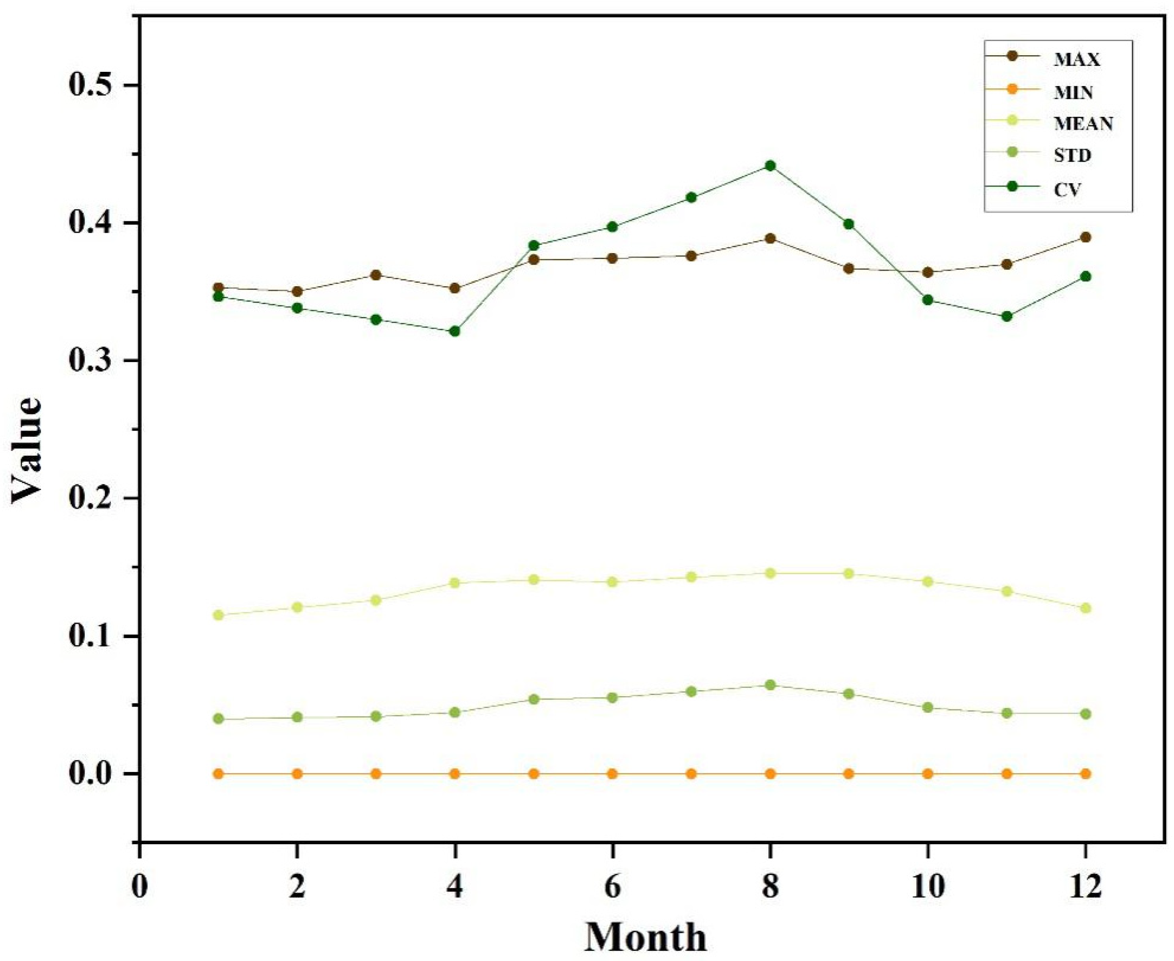
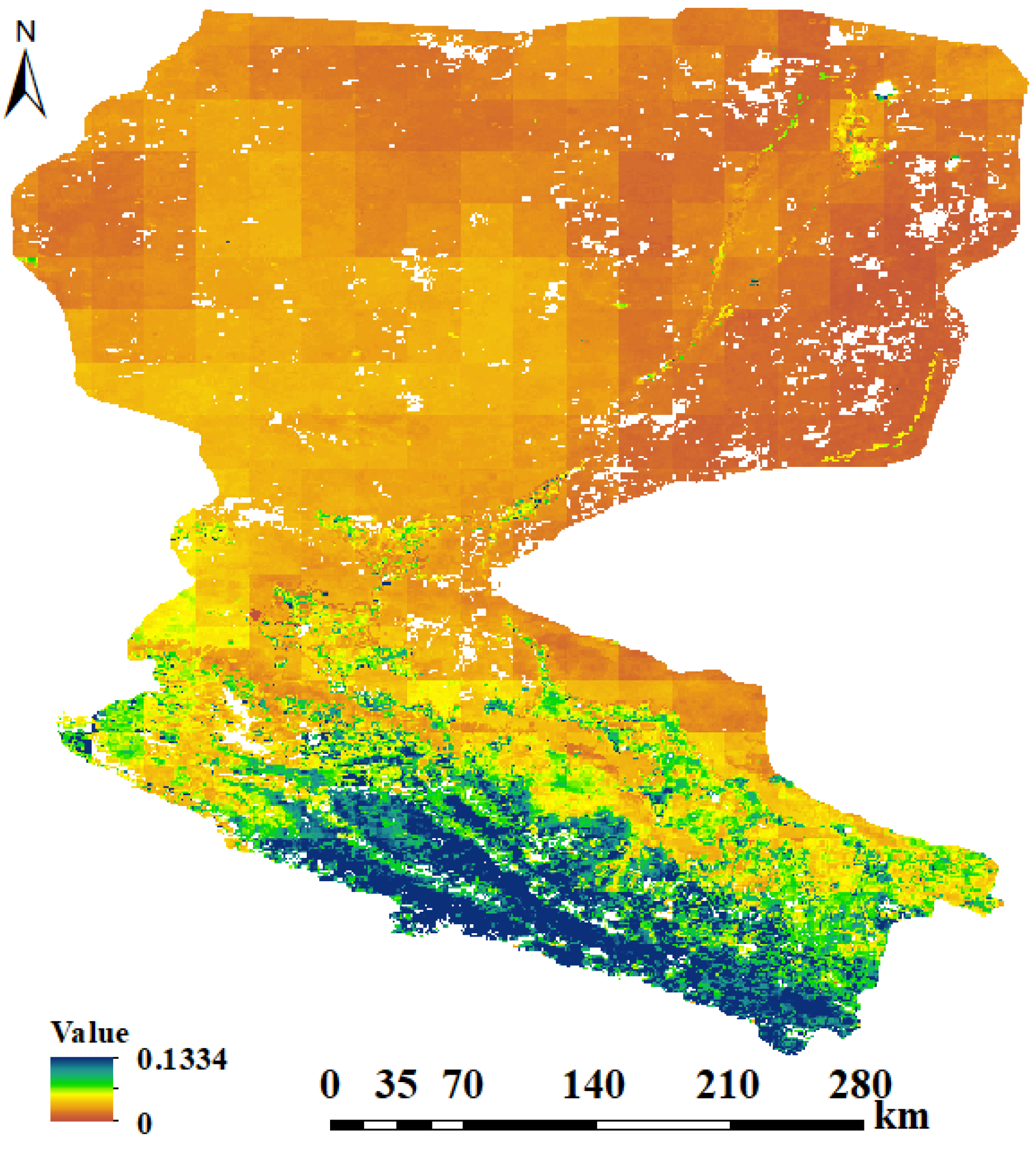
Based on the SM spatial downscaling method proposed by Zhang et al. [25], we obtained a daily 1 km SM dataset for the entire year of 2020. To ensure the reliability of downscaled results, this study employed a random sampling method to generate 1000 pixel points as samples within the Heihe River Basin. The downscaled results were compared with the published 1km SMCI soil moisture products on 15 January, 15 April, 15 July, and 15 October. It was observed that the scattered points were relatively evenly distributed around the 1:1 line, indicating a good correlation between the downscaled results and the SMCI products (Figure 2). The validation results mentioned above demonstrate that the downscaled soil moisture in this study can provide reliable information and can be used for subsequent spatiotemporal analysis. In previous SM analyses, long time series data were often used for analysis, with a better temporal scale, and these studies mainly focused on annual averages [25,70,71,72,73]. However, we found that SM and some of its driving factors exhibit significant temporal variability in this research. In temperate continental climate zones, like the Heihe River Basin, the driving factors vary dramatically during the different seasons and even different months. Therefore, using annual average SM data alone cannot meet research requirements. In response, we focused on the monthly temporal scale of SM patterns and driving factor analysis, and we synthesized the dataset with respect to monthly averages. Figure 3 shows the spatial distribution of the downscaled monthly SM, and Figure 4 shows the basic statistical characteristics of SM in the study area for each month.

3.1. Spatiotemporal Heterogeneity and Stability of Soil Moisture in Heihe River Basin

Based on the SM statistical results, the ratio between the interquartile range and standard deviation of SM for each month ranges from 1.28 to 1.40, and the scatter points in the QQ plot align closely along a straight line. Therefore, it can be concluded that the downscaled SM data approximates a normal distribution, allowing for the next semivariogram function analysis step. Specific semivariogram analysis results are presented in Table 3. In this study, the R2 values of the fitted models range from 0.85 to 0.97, indicating good fits for the corresponding models with relatively small RSS values. The sill values, in general, exhibit a convex distribution. Compared to that in other months, this suggests that SM from May to September exhibits a larger random error, and its distribution is more greatly affected by random errors. This finding indirectly indicates that the spatial variability in SM is higher during this period. Additionally, the sill values of the fitted models exhibit a roughly convex distribution, but there is a significant decrease in July. This suggests that the SM variability in July is lower than that in the neighboring months. The main reason for this phenomenon may be due to the temperate continental climate of the study area. During summer months, there is higher precipitation, and various driving factors intensify the spatial heterogeneity in SM. In contrast, July experiences abundant heat and precipitation, leading to relatively homogeneous SM contents, especially in the middle and lower reaches of the Heihe River Plain. Furthermore, the range values are larger in March, October, and November than in the other months, indicating that SM presents higher spatial variability in these months. Concerning the nugget–sill ratio, the pattern is similar to that of sill values. The nugget–sill ratio is higher in the summer months, indicating that random factors play a dominant role in determining the spatial variability. In contrast, in the winter months, the nugget–sill ratio is lower, suggesting that structural factors are more important for spatial variabilities.
Furthermore, to examine the temporal stability of SM, we categorized SD into five classes based on certain criteria: very poor (SD > 0.2), poor (0.13 < SD < 0.2), stable (0.08 < SD < 0.13), good (0.03 < SD < 0.08), and excellent (SD < 0.03) [23]. This classification was used to explore the temporal stability of SM in the study area. Specifically, in the upper reaches of the basin, the time series SD varies between 0.03 and 0.13, while in the middle and lower reaches, it varies between 0 and 0.03. The overall SD values in the study area are relatively low, with the SD value in the middle and lower reaches being lower than that in the upper reaches. The main reason for this pattern is that the study area belongs to a temperate continental climate with relatively low annual precipitation levels. The overall vegetation cover is limited, and water circulation capacities are relatively low. As a result, the overall temporal stability of SM in the basin is satisfactory. Furthermore, the higher vegetation cover in the upper reaches than that in the middle and lower reaches results in lower SM sensitivity in the middle and lower reaches relative to vegetation seasonal variations. Therefore, the middle and lower reaches exhibit higher temporal stability in SM than in the upper reaches (as shown in Figure 5). In summary, the study area shows significant spatial variability in SM, but the overall monthly scale temporal stability is favorable, and the types of driving factors of SM remain relatively stable across the different months [74].

3.2. Driving Factors of Soil Moisture in Heihe River Basin: Factor Detector

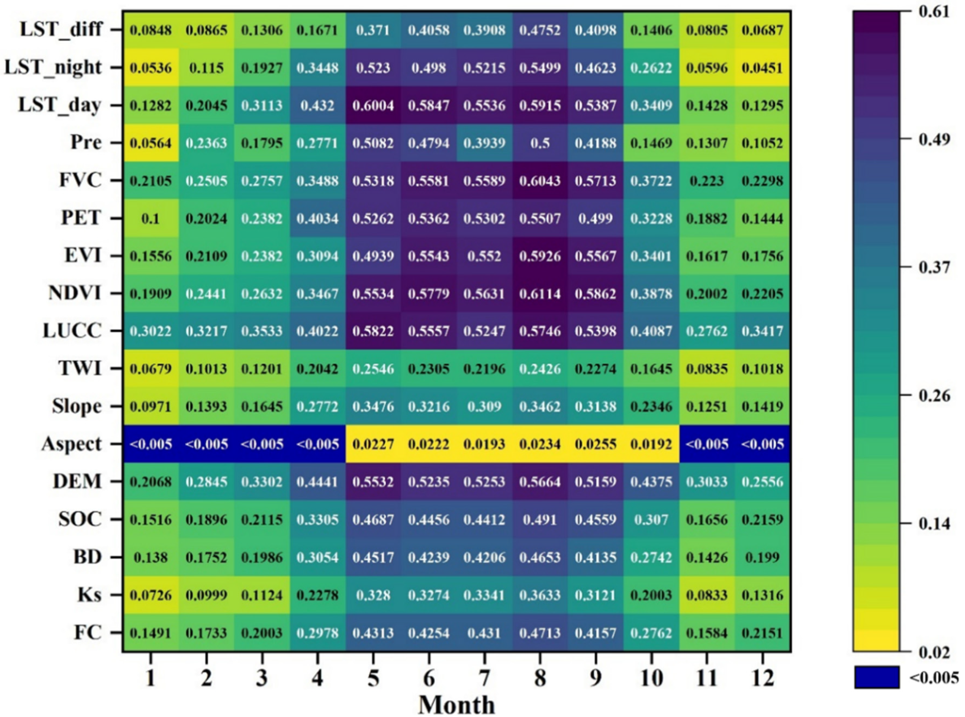
The factor detector results for different months are shown in Figure 6. It can be observed that from January to April and from October to December, the overall q values are relatively low, with the highest q values ranging from approximately 0.3 to 0.45. In these months, land use and land cover (LUCC) is the dominant driving factor of the spatial distribution of SM, especially from January to March and December. Additionally, factors such as elevation, FVC, and NDVI exhibit relatively high q values during these months. In April, October, and November, the primary driving factor is elevation, followed by LUCC, FVC, NDVI, and other factors. During the late spring, summer, and early autumn seasons in the study area, the driving factors impose a greater influence on SM. During the period from May to September, factors such as daytime LST, nighttime LST, vegetation parameters (NDVI, EVI, and FVC), PET, and LUCC show a significant driving power, with q values generally exceeding 0.5. In May, the q value of the daytime LST is the highest at 0.6004, while in August, the q value of the NDVI is the highest at 0.6114, indicating that these factors provide the highest explanatory power for SM in their respective months.
Compared to those of the aforementioned driving factors, soil texture and structure, as well as terrain characteristics, exhibit lower q values. From January to March and in November and December, their q values are generally below 0.2. However, from May to September, the q values vary between 0.3 and 0.5, indicating a higher explanatory power that is still significantly lower than that of driving factors such as daytime LST, nighttime LST, vegetation parameters (NDVI, EVI, and FVC), PET, and LUCC during the same seasons. It is important to note that aspect exhibits an extremely weak driving effect in all months, and its explanatory power for SM significantly deviates from that of the other driving factors. Therefore, at the watershed scale, the 1 km resolution aspect data do not provide a high explanatory power for SM in the study area.
Based on the seasonal division in the Northern Hemisphere (spring: March, April, and May; summer: June, July, and August; autumn: September, October, and November; winter: December, January, and February), it can be observed that the months with lower q values are concentrated in early spring, late autumn, and winter. Considering the research of Luo et al. [26] and the Chinese Permafrost Map (doi:10.12072/ncdc.Westdc.db0029.2021), this could be related to the seasonally frozen soil in temperate continental climates. Specifically, there are two main reasons for this phenomenon. First, the SM downscaling algorithm relies on coarse-scale SM data, which can limit the accuracy of the SM dataset in areas with seasonally frozen soil. Second, the modeling of the relationship between SM and heat is primarily based on liquid SM. However, in the months with lower q values, there may be seasonally frozen soil, rendering the previously established soil–heat relationship no longer applicable. Moreover, in geographical detector analysis, empirical driving factors may not fully match experimental requirements. In the study of Luo et al. [26] on the spatial variation in SM in the Northern Hemisphere, they divided the study seasons into frozen soil seasons and nonfrozen soil seasons, arriving at similar conclusions to those of this study. This suggests that the frozen soil season and vegetation growth conditions could serve as seasonal difference factors of the factor explanatory power in this watershed. Furthermore, compared to the continental-scale study of Luo et al. [26] on SM variations, this watershed-scale study yields larger differences.

3.3. Driving Factors of Soil Moisture in Heihe River Basin: Interaction Detector

To better understand whether the spatial distribution of SM is influenced by the interaction among multiple driving factors, we also used the interaction detector to analyze the impact of the interactions between different influencing factors on SM (Figure S1). On a monthly basis, in January, February, and March, the interaction-detector-based q value was the highest for the combined effect of LUCC and elevation, with a q value of approximately 0.4. From May to September, the interaction detector values generally indicated a higher explanatory power for SM, and the most influential factors were the interaction between vegetation information and other factors, with q values generally exceeding 0.68. During the frozen soil season, the interaction between LUCC and elevation or other factors provided a higher explanatory power for SM, while during the nonfrozen soil season, the interaction between vegetation information and other factors provided higher explanatory power. This suggests that when studying the driving forces of SM with the interaction detector method, the commonly used annual average method overlooks the differences in driving factors during different seasons along the time series. By dividing the seasons into the frozen soil season (or growing season) and the nonfrozen soil season, more precise conclusions can be drawn. However, regardless of the season, the spatial variation in SM was not driven by a single environmental factor; instead, it resulted from the interaction among multiple influencing factors.
Notably, the single-factor q values for aspect, Pre, LST_night, and LST_diff are mostly below 0.1, indicating that they impose very weak individual driving effects on SM. However, these factors exhibit an enhanced effect on SM when interacting with other factors; in particular, aspect shows the most representative result. Across all months of the year, aspect alone exerted a very weak driving force effect on SM, but it showed a significant nonlinear enhancement when interacting with other factors. This study offers a reasonable interpretation of this phenomenon. In a finer-scale study area with relatively lush vegetation growth, the single-factor driving force of aspect on SM may be manifested as different influences on SM between shaded slopes and sunlit slopes (aspect-related effects). However, in this study with an initial SM scale of 1 km, considering the modifiable areal unit problem (MAUP), the sampling interval of the point samples was approximately 8 km. At this scale, the driving force of aspect on other factors is low. The interaction with other factors, such as LST, vegetation conditions, and soil properties, may ensure a more reasonable analysis. It is important to note that while we identified the above pattern, we did not explore the underlying physical mechanisms, so there are limitations. Furthermore, it should be noted that aspect exhibits a phenomenon of single-factor nonlinear attenuation when interacting with the NDVI in February, LUCC in April, and FVC in July. In this study, we did not investigate the patterns and physical reasons for these occurrences, so a reasonable explanation could not be provided.

4. Conclusions

In this study, we first generated a 1 km SM dataset via downscaling and employed geostatistical analysis and the optimized parameter geographical detector model to investigate the spatiotemporal patterns and driving factors of SM in the Heihe River Basin. The results revealed that the average SM in the study area ranges from 0.115 to 0.146 across different months, indicating a relatively low SM content overall. Regarding spatial distributions, areas with high SM contents were concentrated in upstream grasslands and farmlands, while low-SM-content areas could be found in the bare soil regions of the middle and lower reaches.
The geostatistical analysis results indicated that the optimal theoretical models for SM differ among various months. Months with higher SM contents exhibited larger random errors and higher SM variability. Additionally, the variogram range exceeded the sampling interval for all months, indicating a significant spatial variability in SM across the basin. Furthermore, there was notable seasonal variation in the geostatistical characteristics of SM, but overall, the stability remained satisfactory, with standard deviations ranging from 0 to 0.13 over time.
The factor detector model results indicated that in months with relatively low SM contents, the overall q values are relatively small, with the maximum q values observed for LUCC and DEM. In contrast, in months with higher SM contents, the overall q values were relatively large, and the maximum q values focused on the NDVI and LST factors. Additionally, different driving factors exerted varying degrees of influence on SM, and soil texture, structure, and topographic features generally exhibited lower performance.
Interaction detector model analyses revealed that the spatial heterogeneity in SM is a result of the interaction among multiple driving factors. Most driving factors exhibited pairwise enhancement, and the aspect factor yielded the smallest q values. However, in many months, aspect exhibited nonlinear enhancement when interacting with other factors, suggesting that at the watershed scale, aspect indeed interacts with other driving factors and exhibits more prominent driving mechanisms.
Nonetheless, this study suffers certain limitations. The SM downscaling method used to obtain daily 1 km resolution data does not adequately consider scale effects, resulting in nonuniform transitional SM spatial distribution maps. To improve accuracy, in the future, geostatistical and driving factor analyses should focus on spatial partitioning based on downscaled results. Meanwhile, we also need to consider dividing the basin into upstream and middle-lower reaches.

Supplementary Materials

The following supporting information can be downloaded at: https://www.mdpi.com/article/10.3390/rs15245768/s1, Figure S1: Interaction detector results for each month.

Author Contributions

Conceptualization: X.S., H.G. and D.Y., methodology and experimental design: D.Y. and H.G., resource provision: Y.Z. (Yongrong Zhang) and Y.Z. (Yanan Zhang), writing original draft: D.Y., review and editing: X.Z. and X.S. All authors have read and agreed to the published version of the manuscript.

Funding

This work was supported in part by the Third Xinjiang Scientific Expedition Program under Grant No. 2022xjkk0402 and the Fundamental Research Funds for the Central Universities.

Data Availability Statement

The authors confirm that the article provides data supporting the results of this study.

Conflicts of Interest

The authors declare no conflict of interest.

References

  1. Pauwels, V.R.N.; Hoeben, R.; Verhoest, N.E.C.; De Troch, F.P.; Troch, P.A. Improvement of TOPLATS-based discharge predictions through assimilation of ERS-based remotely sensed soil moisture values. Hydrol. Process. 2002, 16, 995–1013. [Google Scholar] [CrossRef]
  2. Western, A.W.; Zhou, S.L.; Grayson, R.B.; McMahon, T.A.; Bloschl, G.; Wilson, D.J. Spatial correlation of soil moisture in small catchments and its relationship to dominant spatial hydrological processes. J. Hydrol. 2004, 286, 113–134. [Google Scholar] [CrossRef]
  3. Dai, A.; Trenberth, K.E.; Qian, T. Relationship with soil moisture and effects of surface warming. J. Hydrometeorol. 2004, 5, 1117–1130. [Google Scholar] [CrossRef]
  4. Koster, R.D.; Dirmeyer, P.A.; Guo, Z.C.; Bonan, G.; Chan, E.; Cox, P.; Gordon, C.T.; Kanae, S.; Kowalczyk, E.; Lawrence, D.; et al. Regions of strong coupling between soil moisture and precipitation. Science 2004, 305, 1138–1140. [Google Scholar] [CrossRef] [PubMed]
  5. Anderson, M.C.; Norman, J.M.; Mecikalski, J.R.; Otkin, J.A.; Kustas, W.P. A climatological study of evapotranspiration and moisture stress across the continental United States based on thermal remote sensing: 2. Surface moisture climatology. J. Geophys. Res. Atmos. 2007, 112, D11112. [Google Scholar] [CrossRef]
  6. Hollinger, S.E.; Isard, S.A. A Soil Moisture Climatology of Illinois. J. Clim. 1994, 7, 822–833. [Google Scholar] [CrossRef]
  7. Dobriyal, P.; Qureshi, A.; Badola, R.; Hussain, S.A. A review of the methods available for estimating soil moisture and its implications for water resource management. J. Hydrol. 2012, 458–459, 110–117. [Google Scholar] [CrossRef]
  8. Bastiaanssen, W.G.M.; Molden, D.J.; Makin, I.W. Remote sensing for irrigated agriculture: Examples from research and possible applications. Agric. Water Manag. 2000, 46, 137–155. [Google Scholar] [CrossRef]
  9. Anctil, F.; Mathieu, R.; Parent, L.E.; Viau, A.A.; Sbih, M.; Hessami, M. Geostatistics of near-surface moisture in bare cultivated organic soils. J. Hydrol. 2002, 260, 30–37. [Google Scholar] [CrossRef]
  10. Bell, K.R.; Blanchard, B.J.; Schmugge, T.J.; Witczak, M.W. Analysis of Surface Moisture Variations within Large-Field Sites. Water Resour. Res. 1980, 16, 796–810. [Google Scholar] [CrossRef]
  11. Teuling, A.J.; Troch, P.A. Improved understanding of soil moisture variability dynamics. Geophys. Res. Lett. 2005, 32, L05404. [Google Scholar] [CrossRef]
  12. Famiglietti, J.S.; Devereaux, J.A.; Laymon, C.A.; Tsegaye, T.; Houser, P.R.; Jackson, T.J.; Graham, S.T.; Rodell, M.; van Oevelen, P.J. Ground-based investigation of soil moisture variability within remote sensing footprints during the Southern Great Plains 1997 (SGP97) Hydrology Experiment. Water Resour. Res. 1999, 35, 1839–1851. [Google Scholar] [CrossRef]
  13. Brocca, L.; Melone, F.; Moramarco, T.; Morbidelli, R. Spatial-temporal variability of soil moisture and its estimation across scales. Water Resour. Res. 2010, 46, W02516. [Google Scholar] [CrossRef]
  14. Torrence, C.; Compo, G.P. A practical guide to wavelet analysis. Bull. Am. Meteorol. Soc. 1998, 79, 61–78. [Google Scholar] [CrossRef]
  15. Das, N.N.; Mohanty, B.P. Temporal dynamics of PSR-based soil moisture across spatial scales in an agricultural landscape during SMEX02: A wavelet approach. Remote Sens. Environ. 2008, 112, 522–534. [Google Scholar] [CrossRef]
  16. Lee, E.; Kim, S. Wavelet analysis of soil moisture measurements for hillslope hydrological processes. J. Hydrol. 2019, 575, 82–93. [Google Scholar] [CrossRef]
  17. Jawson, S.D.; Niemann, J.D. Spatial patterns from EOF analysis of soil moisture at a large scale and their dependence on soil, land-use, and topographic properties. Adv. Water Resour. 2007, 30, 366–381. [Google Scholar] [CrossRef]
  18. Perry, M.A.; Niemann, J.D. Analysis and estimation of soil moisture at the catchment scale using EOFs. J. Hydrol. 2007, 334, 388–404. [Google Scholar] [CrossRef]
  19. Wang, J.F.; Zhang, T.L.; Fu, B.J. A measure of spatial stratified heterogeneity. Ecol. Indic. 2016, 67, 250–256. [Google Scholar] [CrossRef]
  20. Wang, J.F.; Li, X.H.; Christakos, G.; Liao, Y.L.; Zhang, T.; Gu, X.; Zheng, X.Y. Geographical Detectors-Based Health Risk Assessment and its Application in the Neural Tube Defects Study of the Heshun Region, China. Int. J. Geogr. Inf. Sci. 2010, 24, 107–127. [Google Scholar] [CrossRef]
  21. Yang, S.M.; Quan, Q.; Liang, W.J.; Liu, T.J. Characteristics of Agricultural Droughts and Spatial Stratified Heterogeneity and Dependence of Dominant Factors in Inner Mongolia Autonomous Region, China. Atmosphere 2021, 12, 1249. [Google Scholar] [CrossRef]
  22. Xu, L.; Du, H.R.; Zhang, X.L. Spatial Distribution Characteristics of Soil Salinity and Moisture and Its Influence on Agricultural Irrigation in the Ili River Valley, China. Sustainability 2019, 11, 7142. [Google Scholar] [CrossRef]
  23. Yang, Z.H.; Zhao, J.; Zhu, G.F.; LIu, J.L.; Guo, W.B.; Huang, Z.H.; Wang, Y.Q. The remote sensing estimation and spatial pattern analysis of soil moisture in the Shiyang River Basin in consideration of vegetation cover affect. Acta Ecol. Sin. 2020, 40, 8826–8837. [Google Scholar]
  24. Song, Y.Z.; Wang, J.F.; Ge, Y.; Xu, C.D. An optimal parameters-based geographical detector model enhances geographic characteristics of explanatory variables for spatial heterogeneity analysis: Cases with different types of spatial data. Giscience Remote Sens. 2020, 57, 593–610. [Google Scholar] [CrossRef]
  25. Zhang, E.M.; Liu, Y.J.; Pan, T.; Tan, Q.H.; Ma, Z.A. Evaluating the Effects of Climate Change and Human Activities on the Seasonal Trends and Spatial Heterogeneity of Soil Moisture. Remote Sens. 2022, 14, 4862. [Google Scholar] [CrossRef]
  26. Luo, P.; Song, Y.Z.; Huang, X.; Ma, H.L.; Liu, J.; Yao, Y.; Meng, L.Q. Identifying determinants of spatio-temporal disparities in soil moisture of the Northern Hemisphere using a geographically optimal zones-based heterogeneity model. ISPRS J. Photogramm. Remote Sens. 2022, 185, 111–128. [Google Scholar] [CrossRef]
  27. Vachaud, G.; Desilans, A.P.; Balabanis, P.; Vauclin, M. Temporal Stability of Spatially Measured Soil-Water Probability Density Function. Soil Sci. Soc. Am. J. 1985, 49, 822–828. [Google Scholar] [CrossRef]
  28. Crave, A.; GascuelOdoux, C. The influence of topography on time and space distribution of soil surface water content. Hydrol. Process. 1997, 11, 203–210. [Google Scholar] [CrossRef]
  29. Qu, W.; Bogena, H.; Huisman, J.A.; Vanderborght, J.; Schuh, M.; Priesack, E.; Vereecken, H. Predicting subgrid variability of soil water content from basic soil information. Geophys. Res. Lett. 2015, 42, 789–796. [Google Scholar] [CrossRef]
  30. Panciera, R. Effect of Land Surface Heterogeneity on Satellite Near-Surface Soil Moisture Observations. Ph.D. Thesis, University of Melbourne, Department of Civil and Environmental Engineering, Carlton, Australia, 2009. [Google Scholar]
  31. Charpentier, M.A.; Groffman, P.M. Soil Moisture Variability within Remote Sensing Pixels. J. Geophys. Res.-Atmos. 1992, 97, 18987–18995. [Google Scholar] [CrossRef]
  32. Moore, I.D.; Burch, G.J.; Mackenzie, D.H. Topographic Effects on the Distribution of Surface Soil-Water and the Location of Ephemeral Gullies. Trans. ASAE 1988, 31, 1098–1107. [Google Scholar] [CrossRef]
  33. Woods, R.A.; Sivapalan, M.; Robinson, J.S. Modeling the spatial variability of subsurface runoff using a topographic index. Water Resour. Res. 1997, 33, 1061–1073. [Google Scholar] [CrossRef]
  34. Wang, T.J.; Wedin, D.A.; Franz, T.E.; Hiller, J. Effect of vegetation on the temporal stability of soil moisture in grass-stabilized semi-arid sand dunes. J. Hydrol. 2015, 521, 447–459. [Google Scholar] [CrossRef]
  35. Shen, Q.; Gao, G.Y.; Hu, W.; Fu, B.J. Spatial-temporal variability of soil water content in a cropland-shelterbelt-desert site in an arid inland river basin of Northwest China. J. Hydrol. 2016, 540, 873–885. [Google Scholar] [CrossRef]
  36. Leng, P.; Li, Z.L.; Duan, S.B.; Gao, M.F.; Huo, H.Y. A practical approach for deriving all-weather soil moisture content using combined satellite and meteorological data. ISPRS J. Photogramm. Remote Sens. 2017, 131, 40–51. [Google Scholar] [CrossRef]
  37. Liu, B.; Zhao, W.Z.; Chang, X.X.; Li, S.B. Response of Soil Moisture to Rainfall Pulse in Desert Region of the Heihe River Basin. J. Desert Res. 2011, 31, 716–722. [Google Scholar]
  38. Salvucci, G.D. Estimating the moisture dependence of root zone water loss using conditionally averaged precipitation. Water Resour. Res. 2001, 37, 1357–1365. [Google Scholar] [CrossRef]
  39. Crow, W.T.; Wood, E.F. Multi-scale dynamics of soil moisture variability observed during SGP’97. Geophys. Res. Lett. 1999, 26, 3485–3488. [Google Scholar] [CrossRef]
  40. Crow, W.T.; Berg, A.A.; Cosh, M.H.; Loew, A.; Mohanty, B.P.; Panciera, R.; de Rosnay, P.; Ryu, D.; Walker, J.P. Upscaling Sparse Ground-Based Soil Moisture Observations for the Validation of Coarse-Resolution Satellite Soil Moisture Products. Rev. Geophys. 2012, 50, RG2002. [Google Scholar] [CrossRef]
  41. Wang, Y.Q.; Yang, J.; Chen, Y.N.; Wang, A.Q.; De Maeyer, P. The Spatiotemporal Response of Soil Moisture to Precipitation and Temperature Changes in an Arid Region, China. Remote Sens. 2018, 10, 468. [Google Scholar] [CrossRef]
  42. Li, X.; Liu, S.M.; Li, H.X.; Ma, Y.F.; Wang, J.H.; Zhang, Y.; Xu, Z.W.; Xu, T.R.; Song, L.S.; Yang, X.F.; et al. Intercomparison of Six Upscaling Evapotranspiration Methods: From Site to the Satellite Pixel. J. Geophys. Res. Atmos. 2018, 123, 6777–6803. [Google Scholar] [CrossRef]
  43. Zhang, A.J.; Liu, W.B.; Yin, Z.L.; Fu, G.B.; Zheng, C.M. How will climate change affect the water availability in the Heihe River Basin, Northwest China? J. Hydrometeorol. 2016, 17, 1517–1542. [Google Scholar] [CrossRef]
  44. Li, Z.L.; Xu, Z.G.; Shao, Q.X.; Yang, J. Parameter estimation and uncertainty analysis of SWAT model in upper reaches of the Heihe river basin. Hydrol. Process. 2009, 23, 2744–2753. [Google Scholar] [CrossRef]
  45. Pan, X.D.; Li, X.; Yang, K.; He, J.; Zhang, Y.L.; Han, X.J. Comparison of Downscaled Precipitation Data over a Mountainous Watershed: A Case Study in the Heihe River Basin. J. Hydrometeorol. 2001, 15, 1560–1574. [Google Scholar] [CrossRef]
  46. Li, X.; Cheng, G.D.; Liu, S.M.; Xiao, Q.; Ma, M.G.; Jin, R.; Che, T.; Liu, Q.H.; Wang, W.Z.; Qi, Y.; et al. Heihe Watershed Allied Telemetry Experimental Research (HiWATER): Scientific Objectives and Experimental Design. Bull. Am. Meteorol. Soc. 2013, 94, 1145–1160. [Google Scholar] [CrossRef]
  47. Zhang, Y.R.; Shang, G.F.; Leng, P.; Ma, C.F.; Ma, J.W.; Zhang, X.; Li, Z.L. Estimation of quasi-full spatial coverage soil moisture with fine resolution in China from the combined use of ERA5-Land reanalysis and TRIMS land surface temperature product. Agric. Water Manag. 2023, 275, 107990. [Google Scholar] [CrossRef]
  48. Li, Q.; Shi, G.; Shangguan, W.; Nourani, V.; Li, J.; Li, L.; Huang, F.; Zhang, Y.; Wang, C.; Wang, D. A 1 km daily soil moisture dataset over China using in situ measurement and machine learning. Earth Syst. Sci. Data 2022, 14, 5267–5286. [Google Scholar] [CrossRef]
  49. Hengl, T.; De Jesus, J.M.; MacMillan, R.A.; Batjes, N.H.; Heuvelink, G.B.M.; Ribeiro, E.; Samuel-Rosa, A.; Kempen, B.; Leenaars, J.G.B.; Walsh, M.G. SoilGrids1km—Global soil information based on automated mapping. PLoS ONE 2014, 9, e105992. [Google Scholar] [CrossRef]
  50. Zhang, Y.G.; Schaap, M.G.; Zha, Y.Y. A High-Resolution Global Map of Soil Hydraulic Properties Produced by a Hierarchical Parameterization of a Physically Based Water Retention Model. Water Resour. Res. 2018, 54, 9774–9790. [Google Scholar] [CrossRef]
  51. Peng, S.Z.; Ding, Y.X.; Liu, W.Z.; Li, Z. 1 km monthly temperature and precipitation dataset for China from 1901 to 2017. Earth Syst. Sci. Data 2019, 11, 1931–1946. [Google Scholar] [CrossRef]
  52. Vereecken, H.; Maes, J.; Feyen, J.; Darius, P. Estimating the soil moisture retention characteristic from texture, bulk density, and carbon content. Soil Sci. 1989, 148, 389–403. [Google Scholar] [CrossRef]
  53. Hugar, G.M.; Sorganvi, V.; Hiremath, G.; Hugar, G.M. Effect of organic carbon on soil moisture. Indian J. Nat. Sci. Int. Bimon. ISSN 2012, 976, 0997. [Google Scholar]
  54. Montzka, C.; Rotzer, K.; Bogena, H.R.; Sanchez, N.; Vereecken, H. A New Soil Moisture Downscaling Approach for SMAP, SMOS, and ASCAT by Predicting Sub-Grid Variability. Remote Sens. 2018, 10, 427. [Google Scholar] [CrossRef]
  55. Jia, D.; Wen, J.; Wang, X.; Wang, Z. Soil hydraulic conductivity and its influence on soil moisture simulations in the source region of the Yellow River―Take Maqu as an example. Sci. Cold Arid Reg. 2019, 11, 360–370. [Google Scholar]
  56. Riihimäki, H.; Kemppinen, J.; Kopecký, M.; Luoto, M. Topographic wetness index as a proxy for soil moisture: The importance of flow-routing algorithm and grid resolution. Water Resour. Res. 2021, 57, e2021WR029871. [Google Scholar] [CrossRef]
  57. Varga, C.; Csiszér, L. The influence of slope aspect on soil moisture. Acta Univ. Sapientiae Agric. Environ. 2020, 12, 82–93. [Google Scholar] [CrossRef]
  58. Jiang, P.; Cheng, L.; Li, M.; Zhao, R.; Duan, Y. Impacts of LUCC on soil properties in the riparian zones of desert oasis with remote sensing data: A case study of the middle Heihe River basin, China. Sci. Total Environ. 2015, 506, 259–271. [Google Scholar] [CrossRef]
  59. Han, Y.; Wang, Y.; Zhao, Y. Estimating soil moisture conditions of the greater Changbai Mountains by land surface temperature and NDVI. IEEE Trans. Geosci. Remote Sens. 2010, 48, 2509–2515. [Google Scholar]
  60. Holzman, M.E.; Rivas, R.; Piccolo, M.C. Estimating soil moisture and the relationship with crop yield using surface temperature and vegetation index. Int. J. Appl. Earth Obs. Geoinf. 2014, 28, 181–192. [Google Scholar] [CrossRef]
  61. Manning, C.; Widmann, M.; Bevacqua, E.; Van Loon, A.F.; Maraun, D.; Vrac, M. Soil moisture drought in Europe: A compound event of precipitation and potential evapotranspiration on multiple time scales. J. Hydrometeorol. 2018, 19, 1255–1271. [Google Scholar] [CrossRef]
  62. Ru, C.; Duan, S.; Jiang, X.; Leng, P.; Gao, M.; Huo, H.; Li, Z. A method for surface soil moisture estimation based on the DTR-FVC space. J. Univ. Chin. Acad. Sci. 2018, 35, 771. [Google Scholar]
  63. Brocca, L.; Filippucci, P.; Hahn, S.; Ciabatta, L.; Massari, C.; Camici, S.; Schüller, L.; Bojkov, B.; Wagner, W. SM2RAIN–ASCAT (2007–2018): Global daily satellite rainfall data from ASCAT soil moisture observations. Earth Syst. Sci. Data 2019, 11, 1583–1601. [Google Scholar] [CrossRef]
  64. Sun, H.; Zhou, B.; Liu, H. Spatial evaluation of soil moisture (SM), land surface temperature (LST), and LST-derived SM indexes dynamics during SMAPVEX12. Sensors 2019, 19, 1247. [Google Scholar] [CrossRef] [PubMed]
  65. Ma, C.F.; Wang, W.Z.; Han, X.J.; Li, X. Soil Moisture Retrieval in the Heihe River Basin Based on the Real Thermal Inertia Method. IEEE J. Sel. Top. Appl. Earth Obs. Remote Sens. 2013, 6, 1460–1467. [Google Scholar] [CrossRef]
  66. Carlson, T.N.; Gillies, R.R.; Schmugge, T.J. An Interpretation of Methodologies for Indirect Measurement of Soil-Water Content. Agric. For. Meteorol. 1995, 77, 191–205. [Google Scholar] [CrossRef]
  67. Fang, B.; Lakshmi, V.; Bindlish, R.; Jackson, T.J. Downscaling of SMAP Soil Moisture Using Land Surface Temperature and Vegetation Data. Vadose Zone J. 2018, 17, 1–15. [Google Scholar] [CrossRef]
  68. Maroufpoor, S.; Bozorg-Haddad, O.; Chu, X.F. Geostatistics: Principles and methods. In Handbook of Probabilistic Models; Elsevier: Amsterdam, The Netherlands, 2020; pp. 229–242. [Google Scholar]
  69. Cao, F.; Ge, Y.; Wang, J.F. Optimal discretization for geographical detectors-based risk assessment. Giscience Remote Sens. 2013, 50, 78–92. [Google Scholar] [CrossRef]
  70. Meng, F.; Luo, M.; Sa, C.; Wang, M.; Bao, Y. Quantitative assessment of the effects of climate, vegetation, soil and groundwater on soil moisture spatiotemporal variability in the Mongolian Plateau. Sci. Total Environ. 2022, 809, 152198. [Google Scholar] [CrossRef]
  71. Han, Y.; Qiao, D.; Lu, H. Spatial-temporal coupling pattern between irrigation demand and soil moisture dynamics throughout wheat-maize rotation system in the North China Plain. Eur. J. Agron. 2023, 151, 126970. [Google Scholar] [CrossRef]
  72. Luo, M.; Meng, F.; Wang, Y.; Sa, C.; Duan, Y.; Bao, Y.; Liu, T. Quantitative detection and attribution of soil moisture heterogeneity and variability in the Mongolian Plateau. J. Hydrol. 2023, 621, 129673. [Google Scholar] [CrossRef]
  73. Zhang, Z.; Yin, H.; Zhao, Y.; Wang, S.; Han, J.; Yu, B.; Xue, J. Spatial heterogeneity and driving factors of soil moisture in alpine desert using the geographical detector method. Water 2021, 13, 2652. [Google Scholar] [CrossRef]
  74. Lin, P.F.; Zhu, X.; He, Z.B.; Du, J.; Chen, L.F. Research progress on soil moisture temporal stability. Acta Ecol. Sin. 2018, 38, 3403–3413. [Google Scholar]
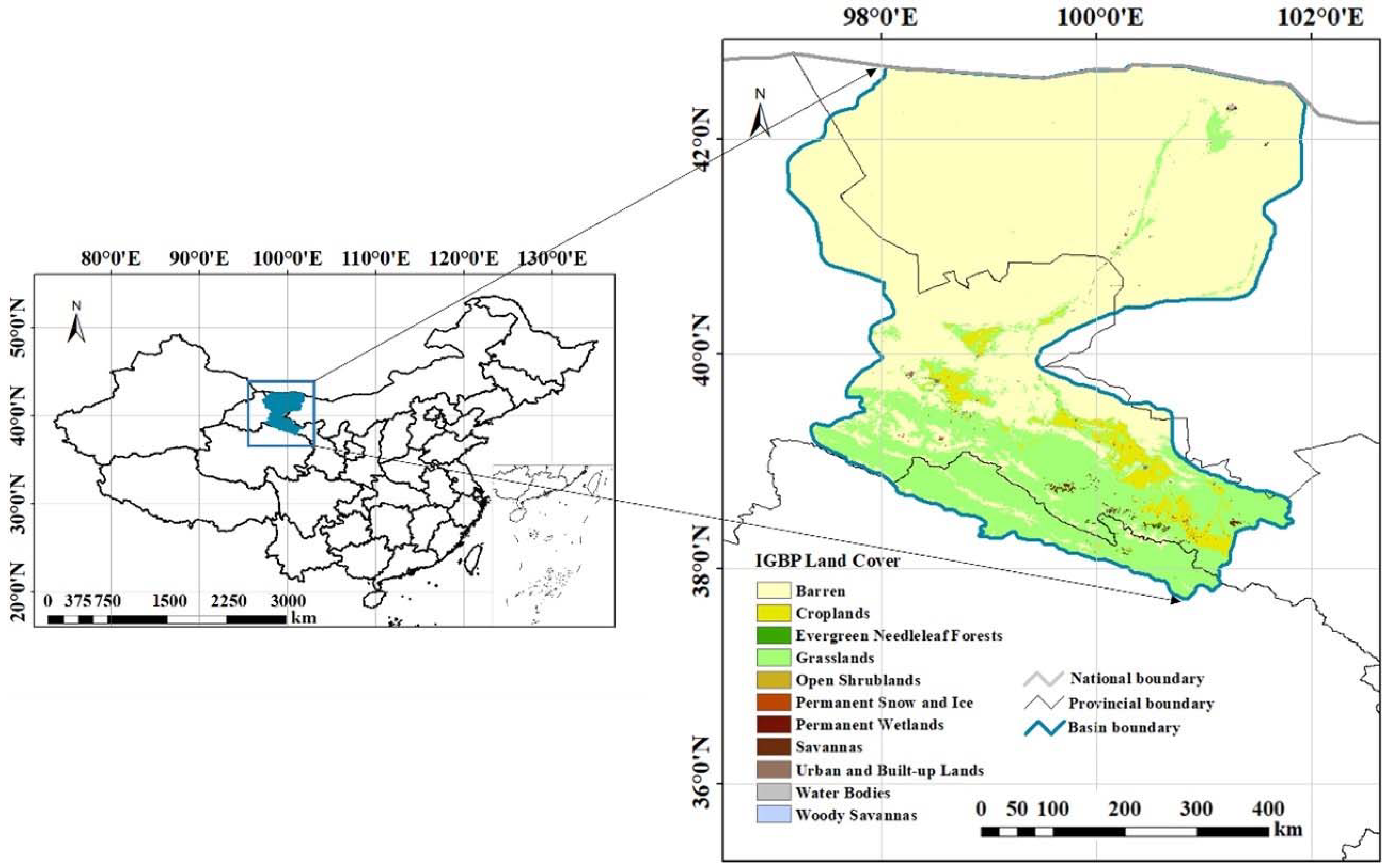
Figure 1. Spatial geographical locations of Heihe River Basin.
Remotesensing 15 05768 g001
Figure 2. Comparison between downscaled SM results and SMCI products.
Remotesensing 15 05768 g002
Figure 3. Monthly average SM downscaling results in the study area.
Remotesensing 15 05768 g003
Figure 4. Monthly statistics of SM in the study area.
Remotesensing 15 05768 g004
Figure 5. Characteristics of SM temporal stability.
Remotesensing 15 05768 g005
Figure 6. The q values of the selected driving factors for each month.
Remotesensing 15 05768 g006
Table 2. Type of interaction between the two driving variables and the dependent variable.
Interaction TypeStandard of Judgment
Nonlinear weaken q ( X 1 X 2 ) < M i n ( q ( X 1 ) , q ( X 2 ) )
Uni-variable weaken M i n ( q ( X 1 ) , q ( X 2 ) ) < q ( X 1 X 2 ) < M a x ( q ( X 1 ) ) , q ( X 2 ) )
Bi-variable enhance q ( X 1 X 2 ) > M a x ( q ( X 1 ) , q ( X 2 ) )
Independent q ( X 1 X 2 ) = q ( X 1 ) + q ( X 2 )
Nonlinear enhance q ( X 1 X 2 ) > q ( X 1 ) + q ( X 2 )
Table 3. Parameters of semi-variance functions for downscaled SM datasets.
MonthModelNuggetSillNugget Coefficient/%Range/mR2RSS
1 Linear0.001030.001730.405263,6960.8736.39 × 10−8
2 Linear0.000980.001760.447263,7020.8817.51 × 10−8
3 Exponential0.000880.003440.7441,833,0000.8511.24 × 10−7
4 Spherical0.000820.002710.699611,0000.8811.64 × 10−7
5 Gaussian0.001150.010620.892908,9800.9691.55 × 10−7
6 Gaussian0.001350.011140.879958,1700.9621.72 × 10−7
7 Spherical0.001290.004910.737611,0000.8736.41 × 10−7
8 Gaussian0.001660.015600.894962,8470.9623.41 × 10−7
9 Gaussian0.001510.011280.866916,7740.9612.05 × 10−7
10 Exponential0.001100.004500.7561,833,0000.8701.88 × 10−7
11 Exponential0.001120.003660.6931,833,0000.8908.60 × 10−8
12 Linear0.001190.001940.384263,7020.9492.69 × 10−8
Disclaimer/Publisher’s Note: The statements, opinions and data contained in all publications are solely those of the individual author(s) and contributor(s) and not of MDPI and/or the editor(s). MDPI and/or the editor(s) disclaim responsibility for any injury to people or property resulting from any ideas, methods, instructions or products referred to in the content.