Article

Temporal and Spatial Surface Heat Source Variation in the Gurbantunggut Desert from 1950 to 2021

1
Institute of Desert Meteorology, China Meteorological Administration, Urumqi 830002, China
2
National Observation and Research Station of Desert Meteorology, Taklimakan Desert of Xinjiang, Urumqi 830002, China
3
Taklimakan Desert Meteorology Field Experiment Station of China Meteorological Administration, Urumqi 830002, China
4
Xinjiang Key Laboratory of Desert Meteorology and Sandstorm, Urumqi 830002, China
5
Key Laboratory of Tree-Ring Physical and Chemical Research, China Meteorological Administration, Urumqi 830002, China
*
Author to whom correspondence should be addressed.
Remote Sens. 2023, 15(24), 5731; https://doi.org/10.3390/rs15245731
Submission received: 17 October 2023 / Revised: 6 December 2023 / Accepted: 8 December 2023 / Published: 14 December 2023

Abstract

:
Based on data from the Gurbantunggut Desert, the largest fixed/semi-fixed desert in China, and ERA5-Land reanalysis data, the long-term variations and spatial surface heat source (SHS) differences in the Gurbantunggut Desert are discussed herein. The results show the following: (1) The hourly SHS at the Kelameili station during the 2013–2021 period was a weak heat source at night; contrastingly, it was a strong heat source during the day. The duration of the hourly SHS increased gradually from January to July, but it decreased gradually from July to December. The daily SHS showed obvious seasonal variation, reaching the maximum in summer and the minimum in winter. The ERA5-Land reanalysis can reproduce all the variation characteristics of the SHS well. (2) The climatology (i.e., multi-year mean) of the monthly SHS intensity was lower than 50 W/m2 during the January–March and September–December periods in the Gurbantunggut Desert, indicating a weak heat source. On the other hand, the climatology recorded in April–August was higher than 50 W/m2, with a strong heat source. From the perspective of spatial distribution, the eastern and western regions of the Gurbantunggut Desert show strong heat sources, while the central region shows weak heat sources. The spatial distribution of the first and second modes of the empirical orthogonal function (EOF) decomposition reflected the consistent spatial variability and a north–south (or east–west) polarity variation of the monthly SHS in the Gurbantunggut Desert, respectively. (3) The yearly SHS showed negative anomalies during the 1950–1954, 1964–1982 and 2004–2015 periods, and positive anomalies during the 1955–1963, 1983–2003 and 2016–2021 periods in the Gurbantunggut Desert. Additionally, the time series of the SHS anomalies was positively correlated with the Interdecadal Pacific Oscillation (IPO) index. During the negative IPO phase, the yearly SHS showed a negative anomaly in the Gurbantunggut Desert, while the yearly SHS showed a positive anomaly during the positive IPO phase in most regions of the Gurbantunggut Desert.

1. Introduction

In the context of global warming, heat forcing and climate events have changed significantly at the regional level [1,2,3]. Desert areas are widely distributed, extreme environments with unique environmental impacts on regional climate change [4]. At the same time, underlying surface conditions such as high albedo and high sand heat capacity efficiency in desert areas comprise typical energy budget characteristics, different from those of other areas [5,6]. In addition, studies have shown that the variation in the surface heat source (SHS) is closely related to large-scale circulation changes, regional climate and monsoons [2,7,8].
Sensible and latent heat fluxes are important components of surface heating, and many studies have been conducted on the spatiotemporal variation characteristics of these components. For instance, the spring surface sensible heat flux in the Tibetan Plateau showed a decreasing trend, but this changed to an increase after approximately the year 2000 [9]. The summer sensible heat flux in the eastern Tibetan Plateau and western Xinjiang in winter showed a decreasing trend, while the other regions showed an increasing trend in China [10,11]. Su et al. [12] found that the summer latent heat flux on the Qinghai–Tibet Plateau from 2000 to 2016 showed an increasing trend, while the sensible heat flux showed an increasing and then decreasing trend. At the same time, sensible heat changes on the Qinghai–Tibet Plateau have an impact on large-scale circulation and monsoon precipitation in the surrounding areas [9,10,13,14]. The sensible and latent heat fluxes on the Qinghai–Tibet Plateau are also closely related to the atmospheric boundary layer height, which is mainly influenced by surface heating [11,12]. For the variation characteristics of the sensible and latent heat fluxes in the desert area of Xinjiang, due to the extremely arid desert climate of the Taklamakan Desert, sensible heat flux is the main form of surface energy consumption, while latent heat flux is relatively low. The increase in summer precipitation in the desert leads to a slight increase in the latent heat flux. However, this does not fundamentally change the status quo according to which the sensible heat flux is the main form of energy consumption in desert ecosystems [15].
Surface heat sources (SHSs) show obvious temporal variation. Guo et al. [16] studied the intensity of SHSs in Shuanghu from October 2011 to September 2012. The results show that although the annual SHS intensity in Shuanghu is basically positive, there were significant seasonal and diurnal variations. In summer and winter, the daytime showed a strong heat source, while the nighttime showed a weak heat source, and the regional-scale precipitation was influenced by abnormal surface heating. Chen et al. [17] analyzed the relationship between the SHSs in the Tibetan Plateau and summer precipitation in the Sichuan Basin during the 1961–1995 period. They found that there was a significant negative correlation between the intensity of SHSs in the Tibetan Plateau in May–June and the intensity of drought in the following year in the Sichuan Basin, along with a significant positive correlation between the intensity of SHS in June and the precipitation anomaly over the Sichuan Basin in June–August in the next year. Hua et al. [7] studied the relationship between vegetation change and SHS and precipitation on the Qinghai–Tibet Plateau. The results show that there was a positive correlation between vegetation and SHS. In other words, after vegetation improvement, the SHS increased in different seasons. They also pointed out that vegetation change caused by the plateau surface heating anomalies may have an impact on summer precipitation in China.
In addition, Duan et al. [8] reviewed and analyzed the response characteristics of East Asian summer precipitation to snow cover and SHSs on the Qinghai–Tibet Plateau. They pointed out that the spring SHS in the plateau mainly affected the “tri-polar” mode of the summer precipitation in East Asia. On the interdecadal scale, the spring SHS was an important cause of “waterlogging in south China and drought in north China” on the Qinghai–Tibet Plateau, while the effect of snow cover in winter was the opposite. At the same time, the Interdecadal Pacific Oscillation (IPO) was also an important cause of “waterlogging in south China and drought in north China” [18,19,20]. In addition, climate events have been shown to correlate with multiple large-scale climate indexes such as the IPO, and the responses of different regions to the large-scale climate indexes were different [21,22,23,24]. Among them, the IPO is a large-scale interdecadal signal based on oceanic/meteorological phenomena with a recurring pattern of sea surface temperatures [25,26]. On interdecadal timescales, sea surface temperatures in the central North and South Pacific cooled (in a positive phase), while the eastern margin and equatorial parts warmed, and vice versa [27].
Previous studies on surface heating anomalies have mainly focused on the Tibetan Plateau. As the second largest desert and the largest fixed/semi-fixed desert in China, the Gurbantunggut Desert is particularly sensitive to climate change due to its unique environment [4]. However, the variation and spatial–temporal distribution characteristics of the surface heating, and its possible linkage to IPO in the Gurbantunggut Desert, are still unclear. In this study, the ability of the European Centre for Medium-Range Weather Forecasts (ECMWF) Reanalysis v5 Land (ERA5-Land) dataset to reproduce observations is evaluated based on the observation data of Kelameili (KLML) station and ERA5-Land reanalysis data. Then, the long-term variation and spatial differences of the SHS in the Gurbantunggut Desert are analyzed. Section 2 introduces the data and methods. Section 3 provides the monthly and yearly temporal–spatial variation characteristics of the SHS in the Gurbantunggut Desert. The discussion and conclusion are presented in Section 4 and Section 5, respectively. The results provide a scientific basis for the study and analysis of the impact of surface heating anomalies on the precipitation, boundary layer height and other factors in desert areas.

2. Data and Method

2.1. Data

The ground-based observation data used in this paper were obtained from the land–air interaction observation station (45.914′08.19″N, 87.935′23.79″E, 531 m above sea level, i.e., the KLML station) built by the Institute of Desert Meteorology, China Meteorological Administration, Urumqi in the KLML area of the Gurbantunggut Desert, encompassing the period of 2013–2021. The hourly upward long-wave radiation, downward long-wave radiation, upward short-wave radiation, downward short-wave radiation and soil heat flux observation data were used to calculate the SHS. The above data were derived from the NR01 four-component radiation sensor (Hukseflux, Delft, The Netherlands) and the HFP01 soil heat flux plate (Hukseflux, Delft, The Netherlands). The data collector adopted CR6 series products from Campbell Company in the United States. The data collection frequency was 1 Hz, and the collection results output average time data and statistical data ranged between 1 s, 10 s, 1 min, 30 min, 1 h, and 1 d.
Solar radiation observation is a routine meteorological observation practice in China. In the process of observation, due to a series of reasons such as the external environment, failures in timely maintenance and the sensitivity of the instrument itself, the accuracy of the observation data declines. Therefore, after obtaining the original data output of the radiation observation system, a series of data processing steps are required. First, obvious outliers are removed. Due to the high sensitivity of the instrument in measuring the short-wave radiation at night, there is an abnormal albedo. In addition, signal transmission or instrument failures can cause garbled data, data loss, a decimal point drift, etc.; therefore, the incomplete data described above were removed first. Then, the missing continuous data within the observation data were interpolated to ensure data continuity by as much as possible. It should be noted that in order to ensure the validity of the average data at different time scales, the missing data with long gaps were removed. For missing data with short gaps, the average of the previous moment and the next moment was used for interpolation. Except for 2019 (where the percentage of valid data was about 73%), the percentage of valid data for the rest of the years following quality control was above 90%.
To investigate the temporal and spatial distribution of the SHSs in the Gurbantunggut Desert, the monthly sensible and sensible heat fluxes were selected from the ERA5-Land reanalysis data during the 1950–2021 period, with a spatial resolution of 0.1° × 0.1° (https://cds.climate.copernicus.eu/cdsapp#!/dataset/reanalysis-ERA5-Land-monthly-means?tab=overview (accessed on 8 January 2023)). Figure 1 shows a schematic diagram of the terrain of the study area and the KLML station [28].
The IPO index was used to investigate the possible relationship between the interdecadal variation characteristics of the SHS and the large-scale circulation anomaly, which was based on the difference between the sea surface temperature anomalies (SSTA) averaged over the central equatorial Pacific and the average of the SSTA in the Northwest and Southwest Pacific. The IPO index was obtained from the U.S. National Oceanic and Atmospheric Administration (NOAA) Physical Sciences Laboratory (https://psl.noaa.gov/data/timeseries/IPOTPI/ (accessed on 8 January 2023)) and is expressed as the annual mean values for the 1950–2021 period in this study [29].

2.2. Methods

2.2.1. Energy Balance Equation

In general, the energy balance equation is expressed as follows [7,16]:
R n G 0 = H + L E
where R n is the net radiation, G 0 is the surface soil heat exchange flux, H is the sensible heat flux and L E is the latent heat flux. The net radiation, R n , is given by
R n = ( D R U R ) + ( D L R U L R )
where D R is the short-wave solar radiation reaching the surface, U R is the reflected short-wave solar radiation, D L R is the long-wave inverse radiation and U L R is the long-wave radiation emitted from the ground. At the KLML station, flux data were obtained based on eddy covariance observations. In general, the energy of the eddy covariance observations system is not conserved in different ecosystems (i.e., R n G 0 > H + L E ) [6,30,31]. Hence, the SHS observed at the KLML station is defined as R n G 0 . Furthermore, ERA5-Land reanalysis products comply with energy conservation (Equation (1)), and the SHS based on the ERA5-Land reanalysis is defined as H + L E [32].

2.2.2. Evaluation Method

The reproducibility of the SHS (calculated according to the sensible and latent heat fluxes) based on the ERA5-Land reanalysis of observations was evaluated according to the mean absolute error (MAE), root-mean-square error (RMSE), R-Square (R2) correlation, quantile–quantile plot (QQ plot), probability density function (PDF) curve and scatter plot.
In this study, the QQ plot and PDF curve were used to verify that the two time series (i.e., observations and ERA5-Land reanalysis) follow the same distribution. Among them, the QQ plot can compare the quantiles and the PDF curve can compare the occurrence probabilities (i.e., frequency) of the two probability distributions [33,34,35]. The QQ plot is defined as follows: assuming that F x is a continuous distribution function of the random variable X (i.e., time series of SHS), then U = F x follows a uniform distribution over the interval (0, 1). Assuming that X t , t X 1 , t is an order statistic for sample X 1 , , X t of a random variable X , let
U k , t = F x k , t
where t is the time and U t , t U 1 , t is an order statistic taken from a uniform distribution over the interval (0, 1). Hence,
E U k , t = E F x k , t = t k + 1 t + 1 , k = 1 , , t
Then, the QQ plot is given as follows:
{ X k , t , F 1 t k + 1 t + 1 : k = 1 , , t }

2.2.3. Empirical Orthogonal Function Analysis of the SHS

Let X ( t ) = [ X 1 ( t ) , , X m ( t ) ] be the SHS data matrix for a given month and X m ( t ) be the t -year time series of the SHS of grid m . Furthermore, it is assumed that X m × t is a linear combination of p spatial eigenvectors and the corresponding time weight coefficients.
Then, the empirical orthogonal function (EOF) is as follows:
X m × t = V m × p T p × n
where T is the time coefficient and V is the spatial eigenvector. In this process, the main information of the variable field is represented by several typical eigenvectors [36,37].

3. Results

3.1. Changes in the Surface Heat Source Ground-Based Observation

To explore the changes in the SHSs at different time scales, Figure 2 shows the average hourly variation in SHS intensity at the KLML station during the 2013–2021 period. It can be seen that the duration and intensity of the SHS increased from January to July and decreased from July to December. From November to February, the hourly SHS intensities were below 175 W/m2, and the maximum diurnal differences were 227 W/m2. The intensities of hourly SHSs were between −115 and 370 W/m2 in March–October, while the maximum intensities of hourly SHSs were about 245–370 W/m2, and the maximum diurnal differences were 485 W/m2. This indicates that the hourly SHS intensity was a strong heat source in March–October and was a weak heat source in November–February; it was a weak heat source at night and a strong heat source during the day.
In addition, the hourly SHS intensities in December–March of each year were significantly different, which was related to the winter snow cover (i.e., more snow reduces surface heating, and vice versa) [8]. At the same time, the hourly SHS showed no obvious differences during June–November of each year, whereby it was low in the morning and evening, and high at noon. The maximum intensity of the SHS occurred at 12:00 in May 2017, reaching 350 W/m2, and the minimum appeared at 12:00 in December 2017. It should be noted that there were missing values from March to May and December 2019.
Figure 3 shows the variation characteristics of the daily, daytime and nightly SHS intensities at the KLML station. To better compare the differences between the daily, daytime and nightly means of the SHS intensity, a 9-day running mean was formulated. It can be seen that the daily variation characteristics of the SHS intensity in each year were consistent. The daily, daytime and night SHS intensities were between −43 and 206 W/m2, −8 and 124 W/m2, and −54 and 23 W/m2, respectively, indicating that the SHS intensity at night was much lower than that at daytime. From January to December, the daily and daytime mean SHS intensities first increased and then decreased, reaching the maximum in summer. However, the opposite was true at night. At the same time, the daily SHS intensity in 2016–2018 was significantly higher than that in the other years. In the winter of 2015 and 2016, the daytime SHS intensity was lower than that at night.
Figure 4 shows the yearly and monthly variations in the SHS intensity at the KLML station. The yearly variations of the daytime SHS intensity showed an upward tendency during 2013–2018 and a downward tendency during 2018–2021 (red line in Figure 4a). As seen in Figure 4b, the SHS intensity showed obvious monthly variations. It was the lowest in winter and the highest in summer. The yearly and monthly variations in the surface energy demonstrated a strong heat source during the daytime and a weak heat source at night.

3.2. Regional-Scale Variation in the SHS

It was necessary to investigate the long-term variation characteristics of the SHS intensity in the Gurbantunggut Desert at the regional scale. However, the time length and spatial resolution of the observation data were limited. Hence, it was necessary to use reanalysis data. First, the reproducibility of the SHS intensity of the ERA5-Land reanalysis in observations was evaluated. Further, the characteristics of long-term spatial–temporal variation in the SHS intensity in the Gurbantunggut Desert were explored based on the ERA5-Land reanalysis data.

3.2.1. Evaluation of the Reproducibility of the ERA5-Land Reanalysis

Before analyzing the temporal and spatial distribution characteristics of the SHS intensity in the Gurbantunggut Desert, the ability of the ERA5-Land reanalysis to reproduce the observation was evaluated. Table 1 outlines the evaluation indexes between the monthly SHS intensity of the observations and the ERA5-Land reanalysis. It can be seen that the RMSE and MAE values between the observation and ERA5-Land reanalysis were 9.56 W/m2 and 8.32 W/m2, respectively, indicating that the deviation and the mean error between observation and ERA5-Land reanalysis were less than 10 W/m2. Moreover, the interannual variations in the observation and ERA5-Land reanalysis were 0.016 W/m2 and −0.013 W/m2, respectively.
At the same time, the R2 was 0.9, meaning that the monthly SHS intensity of the ERA5-Land reanalysis could explain 90% of the variation in the observation, and the tendency of the monthly SHS intensity of the ERA5-Land reanalysis was notably consistent with the observation (i.e., the correlation was 0.96 and significant at the 0.05 significance level). These values indicate that ERA5-Land reanalysis can effectively reproduce all the variation characteristics of the monthly SHS intensity.
Furthermore, in order to compare the differences in the probability distributions and time series of the monthly SHS intensity between the observation and the ERA5-Land reanalysis during 2013–2021 more intuitively, Figure 5 depicts the QQ plot, PDF curve, scatter plot and time series.
Figure 5a shows the empirical quantiles of the monthly SHS intensity of the observation and ERA5-Land reanalysis. It can be seen that the monthly SHS intensity of the ERA5-Land reanalysis, which was between 0 and 50 W/m2, was basically consistent with the observations, while the monthly SHS intensity, which was over 50 W/m2, was lower than the observation, with a deviation within 20 W/m2. The variation in the PDF curve of the monthly SHS intensity of the ERA5-Land reanalysis was basically consistent with the observation, but the frequency between 0 and 70 W/m2 was more than that of the observation, and the frequency above 70 W/m2 was less than that of the observation (Figure 5b). The ERA5-Land reanalysis can reproduce the probability distribution characteristics of the monthly SHS intensity well, and the deviation was small. At the same time, the correlation coefficient between the ERA5-Land reanalysis and observation reached 0.96. The scatter plot was almost diagonal and the time series coincided, indicating that ERA5-Land reanalysis could effectively reproduce the time variation characteristics of the observed monthly SHS intensity (Figure 5c,d). In conclusion, although there was a small deviation, the ERA5-Land reanalysis can effectively reproduce the variation characteristics of the monthly SHS intensity at the KLML station.

3.2.2. Changes in the Monthly SHS Intensity in the Gurbantunggut Desert

The ERA5-Land reanalysis can reproduce the variation characteristics of SHS intensity at the KLML station well. Furthermore, the long-term variation and spatial distribution characteristics of the SHS intensity in the Gurbantunggut Desert were analyzed using the reanalysis data. Figure 6 demonstrates the spatial distribution of the monthly SHS intensity in the Gurbantunggut Desert in 1950–2021. It can be seen that the SHS intensity of each month showed the spatial distribution characteristics of “high in the south and low in the north”. Combined with the topography in Figure 1, the northern part of the desert was close to the Altay Mountains, while the southern part was close to the urban agglomeration. Human activities in urban clusters may affect the variation in the SHS intensity in the southern desert. The SHS intensity in the Gurbantunggut Desert was lower than 50 W/m2 and showed a weak heat source in January–March and September–December. Additionally, the SHS intensity was higher than 50 W/m2 and showed a strong heat source in April–August. Simultaneously, the SHS intensity showed obvious monthly variation, reaching the maximum in May–July, with the maximum exceeding 90 W/m2. In addition, the SHS intensity in the desert hinterland was lower than that in the surrounding areas during April–August.
Furthermore, the temporal and spatial variation characteristics of the SHS intensity were investigated based on the EOF analysis in the Gurbantunggut Desert. Figure 7 shows the spatial distribution of the first and second modes of the EOF (i.e., EOF1 and EOF2) decomposition of the SHS intensity in the Gurbantunggut Desert from January to December. It can be seen that the explanatory variance in the first mode in each month exceeded 50%, and the explanatory variance in the first mode of the SHS intensity in September reached 81.34%. These indicate that the first mode dominated the variation in the SHS intensity in the desert region. From the spatial distribution of EOF1 in each month, it can be seen that the eigenvalues of the desert regions were all positive (or negative), indicating that the change in the SHS intensity was consistent (i.e., the spatial variability in the SHS intensity was consistent), reflecting the consistent-phased distribution characteristics of the SHS intensity.
The interpretive variance of EOF2 ranged from 6.23 to 15.6%, and the spatial distribution of EOF2 presented a north–south or east–west polarity variation in each month. In January and November, the SHS intensity showed a north–south reverse change, while the other months showed an east–west reverse change. At the same time, the reverse variation difference of the SHS intensity was the same from May to August.
Figure 8 displays the time coefficient of the first two modes of the EOF decomposition of the SHS intensity in the Gurbantunggut Desert in each month. It can be seen that the variation characteristics of the first mode of the SHS intensity in Gurbantunggut were quite different in each month. Among them, the SHS intensities in January, March, July, August and November showed obvious interdecadal variation. As seen in Figure 8a, the SHS intensity in the Gurbantunggut Desert in January showed an upward tendency from the 1950s to the mid-1960s, and from the mid-1990s to the early 2010s, while they showed a downward tendency from the mid-1960s to the mid-1990s and from early 2010s until now. Compared with the time coefficient of the first mode, the time coefficient of the second mode of the SHS intensity showed interannual variability.

3.2.3. Changes in the Yearly SHS Intensity in the Gurbantunggut Desert

The long-term variations in the yearly SHS intensity in the Gurbantunggut Desert were analyzed. Figure 9 shows the spatial distribution of climatology (i.e., multi-year mean), trend and time series of the yearly SHS intensity in the Gurbantunggut Desert during the 1950–2021 period. As shown in Figure 9a, the climatology of the yearly SHS intensity in the Gurbantunggut Desert was between 34 and 58 W/m2, and the yearly SHS intensity was lower in the central part and higher in the western and eastern parts. Among them, the climatology of the yearly SHS intensity in the central part was between 34 and 44 W/m2, while it was between 44 and 58 W/m2 in the western and eastern parts. In addition, the time series of the anomalies of the yearly SHS intensity showed obvious interdecadal variation characteristics (Figure 9c). As shown in Table 2, the time series of the yearly SHS intensity showed negative anomalies at P1, P3 and P5, and showed positive anomalies during at P2, P4 and P6.
Figure 10 also shows the spatial distribution and the time coefficients of the first two modes of the EOF decomposition of the yearly SHS intensity in the Gurbantunggut Desert. The explanatory variance in the first mode of the yearly SHS intensity exceeded 75.44%, and the eigenvalues of EOF1 of the yearly SHS were positive, indicating that the change in the yearly SHS intensity was consistent (i.e., the spatial variability in the yearly SHS intensity was consistent). The time coefficient of the first mode of the yearly SHS intensity showed interdecadal variability, and the variation characteristics were consistent with the yearly SHS intensity anomalies (Figure 10c). Looking at Figure 10a,c, it can be seen that the interdecadal variation in the yearly SHS intensity presents consistent positive or negative anomalies in spatial distribution in the Gurbantunggut Desert. As shown in Figure 11, the yearly SHS intensity showed negative anomalies at P1, P3 and P5, and positive anomalies at P2, P4 and P6 in the Gurbantunggut Desert.
The explanatory variance in the second mode of the yearly SHS intensity exceeded 7.72%, and the spatial distribution of EOF2 of the yearly SHS intensity presented an east–west polarity variation (Figure 10b). Before the mid-1990s, the change in the time coefficient of the second mode was relatively smooth. From the mid-1990s to the early 2000s, the time coefficient showed an upward tendency, whereas since the early 2000s, it has shown a downward tendency (Figure 10d).

3.2.4. Possible Linkage between the SHS Intensity and Interdecadal Pacific Oscillation

As mentioned in the previous section, the anomalies in yearly SHS intensity in the Gurbantunggut Desert over recent decades have shown obvious interdecadal variation. Therefore, the possible linkage between the SHS intensity and IPO was explored in this section. Figure 12 shows the time series of the SHS intensity anomalies and IPO index during the 1950–2021 period. The IPO was in a negative phase in 1950–1976 and 1999–2021, and a positive phase in 1977–1998 (Figure 12b). Moreover, the time series of the SHS intensity anomalies was positively correlated with the IPO index, with a correlation coefficient of 0.34 (significant at the 0.05 level).
Figure 13 depicts the spatial distribution of the yearly SHS intensity anomalies in the Gurbantunggut Desert during the different IPO phases. In the negative IPO phase, the yearly SHS intensity showed a negative anomaly in the Gurbantunggut Desert. In the positive IPO phase, the yearly SHS intensity in the western part of the Gurbantunggut Desert presented a negative anomaly, while the other regions of the Gurbantunggut Desert presented a positive anomaly.
Further, Figure 14 depicts the spatial distribution characteristics of precipitation anomalies in different IPO periods in northern Xinjiang. It can be seen that the precipitation anomaly in northern Xinjiang was less in the IPO negative phase, and more in the IPO positive phase. This result is supported by the previous studies [24]. The precipitation anomaly in northern Xinjiang was positively correlated with the SHS intensity (corr = 0.44 and significant at the 0.05 level), negatively correlated with the sensible heat flux (corr = −0.84 and significant at the 0.05 level), and positively correlated with the latent heat flux (corr = 0.90 and significant at the 0.05 level) at KLML station. The main form of latent heat flux was the phase transition of water. Hence, the change in the latent heat flux was greater than that in the sensible heat flux when there was more precipitation in the desert, and this led to an increase in the intensity of the SHS (i.e., positive IPO phase). The opposite was true when precipitation was low.

4. Discussion

The SHS was a weak heat source at night and a strong heat source during the daytime, and the intensity of the SHS increased gradually from January to July but decreased gradually from July to December at the KLML station. At the same time, the long-term temporal and spatial variation characteristics of the SHS intensity in the Gurbantunggut Desert are discussed based on the ERA5-Land reanalysis. The EOF1 of each month showed changes in the form of the consistent strengthening or weakening of the SHS intensity in desert areas. The spatial distribution of EOF2 in each month showed a north–south or east–west polarity variation. The variation characteristics of the time coefficients of each mode were different in each month.
In addition, the seasonal and diurnal variations in the SHS intensity at the KLML station were consistent with those in the central Qiangtang Plateau [16]. With the increase in vegetation on the Qinghai–Tibet Plateau, the SHS intensity in this plateau also increased in general [38]. However, as the largest fixed/semi-fixed desert in China, the SHS intensity of the Gurbantunggut Desert has not significantly increased or decreased over recent decades. At the same time, the contribution of the latent heat flux to the SHS intensity in the Gurbantunggut Desert was greater than that in the central and western Tibetan Plateau and the Taklimakan Desert [39].
Studies have pointed out that sensible and latent heat fluxes are among the main factors affecting the height change in the atmospheric boundary layer. The sensible heat flux, latent heat flux, atmospheric boundary layer height, monsoon, monsoon precipitation, large-scale circulation, etc., affect and restrict one another [12,40,41,42,43]. Anomalies in the SHS intensity on the Qinghai–Tibet Plateau have an impact on the Asian Summer Monsoon and summer precipitation in eastern China [7,8]. The Pacific Ocean SSTA (i.e., IPO) and the spring SHS intensity on the Qinghai–Tibet Plateau were important causes of “waterlogging in south China and drought in north China” [8,24]. These studies indicate that the surface energy variation is closely related to large-scale circulation. However, regarding the variations in surface energy, the possible mechanisms underlying interdecadal variation in the SHS intensity anomalies and the relationship between the SHS intensity anomalies in the Gurbantunggut Desert, and the precipitation change in the surrounding area and Eastern China, remain unclear. Therefore, exploring the long-term variation characteristics of SHS intensity in the Gurbantunggut Desert provides scientific theoretical support for further research on the mechanisms of the weather and climate events in northern Xinjiang, and even the whole Xinjiang region.

5. Conclusions

In this study, based on the observation data of the KLML station and ERA5-Land reanalysis, the reproducibility of the ERA5-Land reanalysis data for observation was evaluated, and the long-term variations and spatial differences in the SHS in the Gurbantunggut Desert were discussed. The results show the following:
(1)
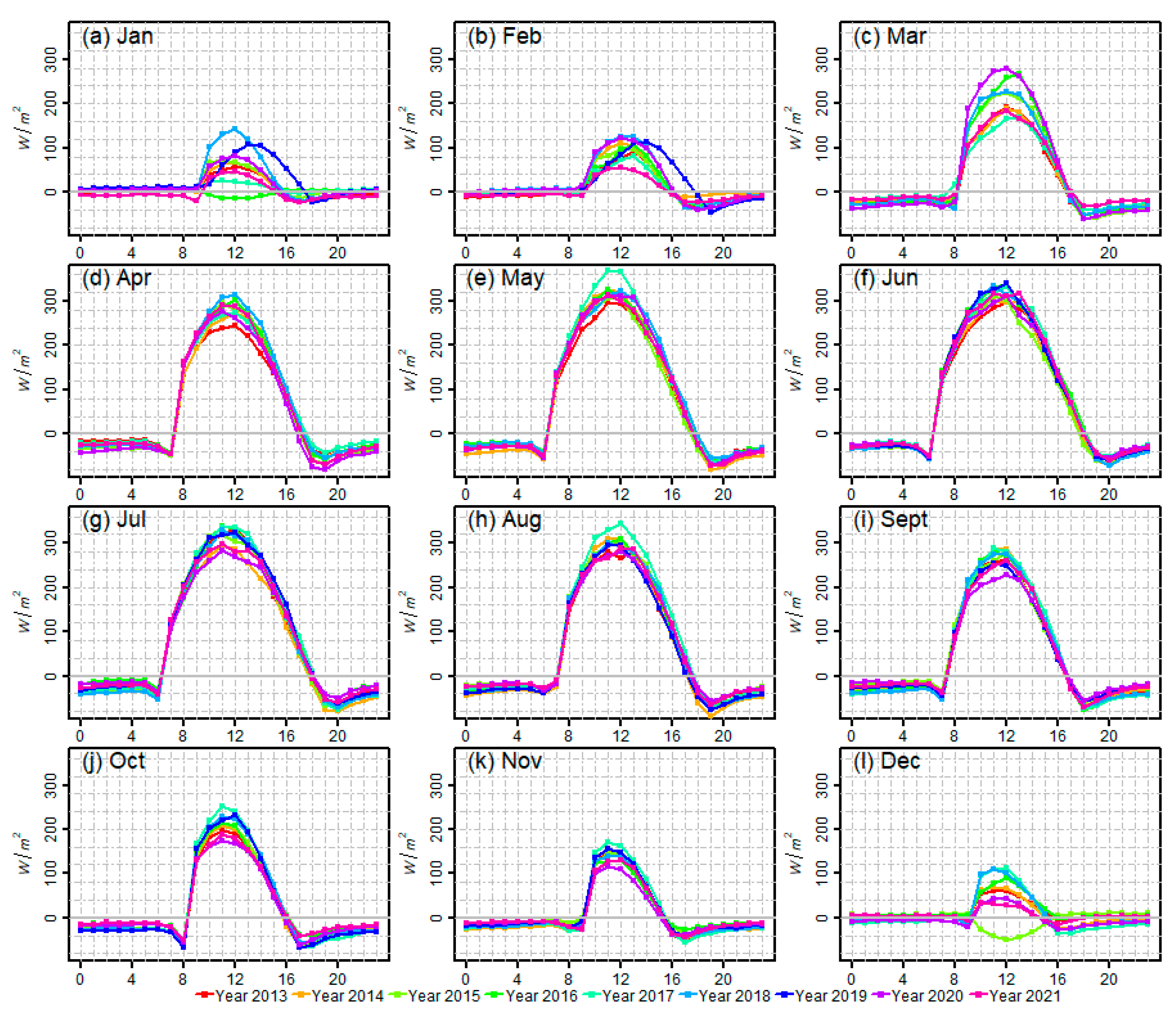
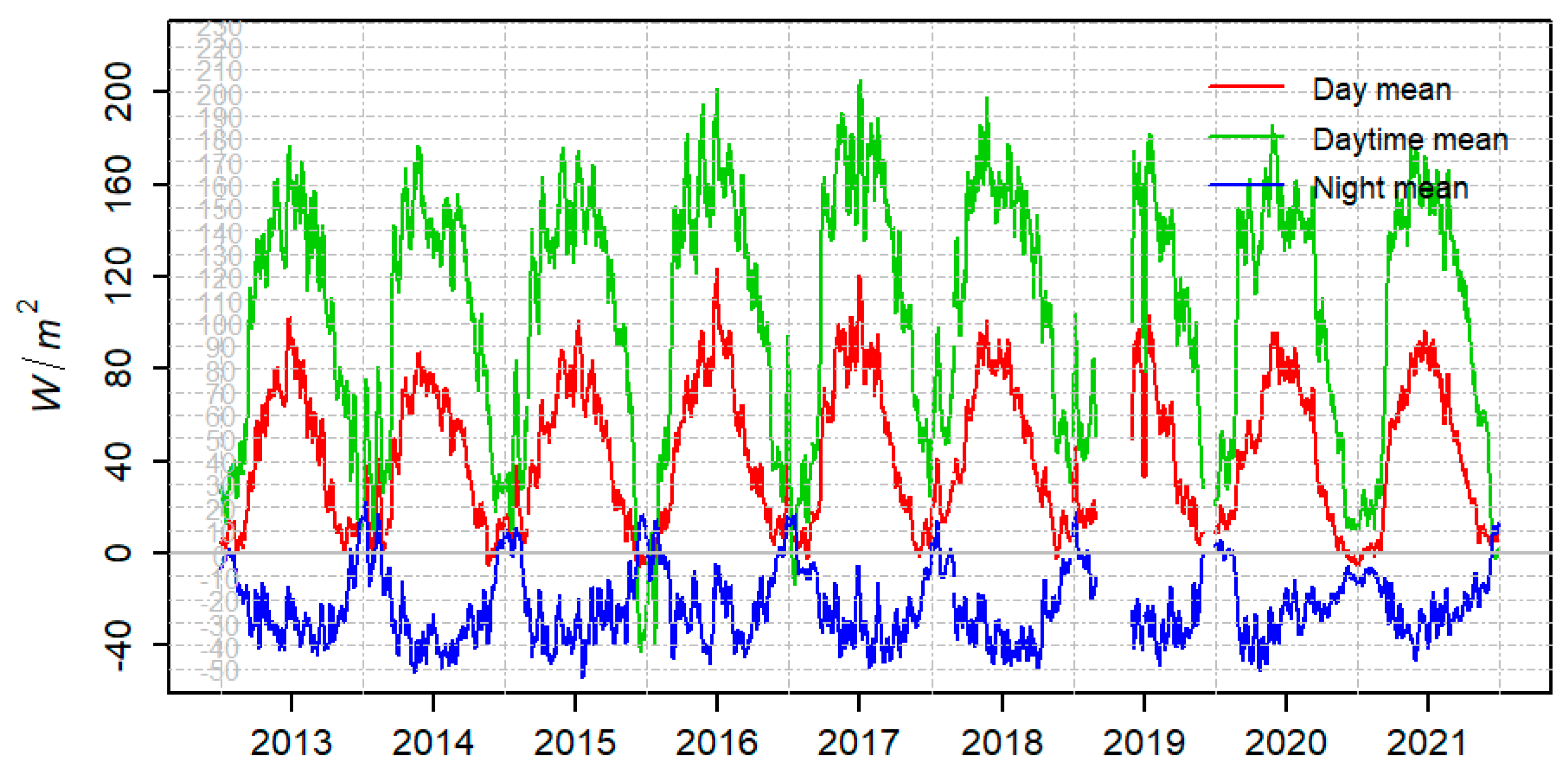
The hourly SHS intensity in the KLML station from 2013 to 2021 showed a gradual increase in duration and intensity from January to July, and a gradual decrease from July to December. It was a weak heat source at night and a strong heat source during the daytime. The characteristics of the daily variation in the SHS intensity in each year were consistent. The daily and daytime SHS intensities showed obvious seasonal variation, and the intensity of the SHS reached the maximum in summer and the minimum in winter, while the intensity of the SHS at night demonstrated the opposite. The annual and monthly variations in the surface energy were a strong heat source during the daytime and a weak cold source at night. From 2016 to 2021, the yearly SHS intensity first decreased and then increased;
(2)
The RMSE and MAE of the monthly SHS intensity between the observation and ERA5-Land reanalysis were all less than 10 W/m2. ERA5-Land reanalysis could explain 90% of the variation (R2) in the observations, and the tendency of the ERA5-Land reanalysis was significantly consistent with the observation (0.05 significance level). The monthly SHS intensity between 0 and 50 W/m2 obtained from the ERA5-Land reanalysis was basically consistent with the observations, while the monthly SHS intensity over 50 W/m2 was lower than seen in the observations. In conclusion, ERA5-Land reanalysis can reproduce the probability distribution characteristics of the monthly SHS intensity well. At the same time, the correlation coefficient between the ERA5-Land reanalysis and observation reached 0.96, the scatter plot was basically diagonal, and the time series coincided, indicating that ERA5-Land reanalysis could reproduce the time variation characteristics of the observed SHS intensity effectively;
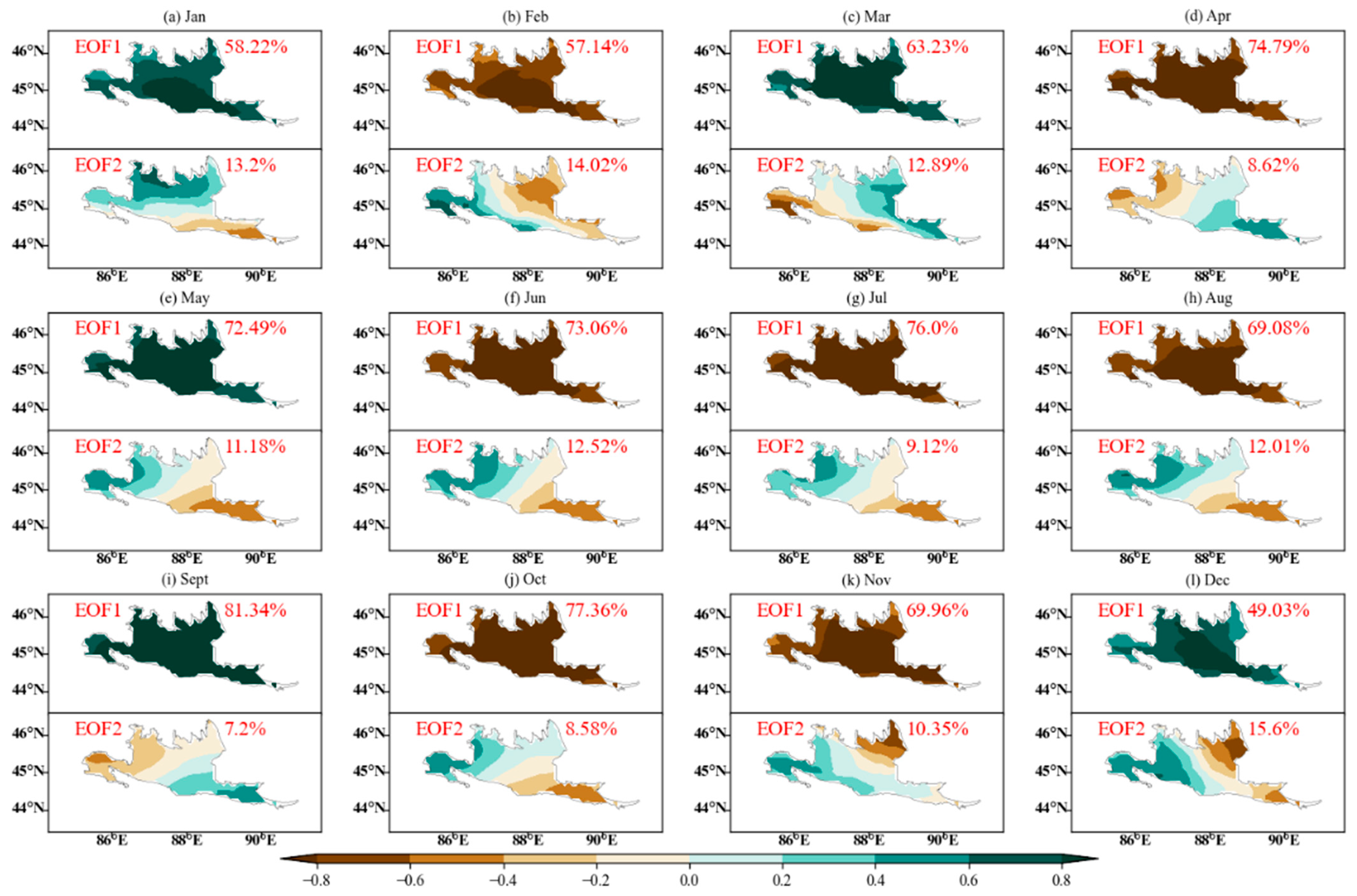
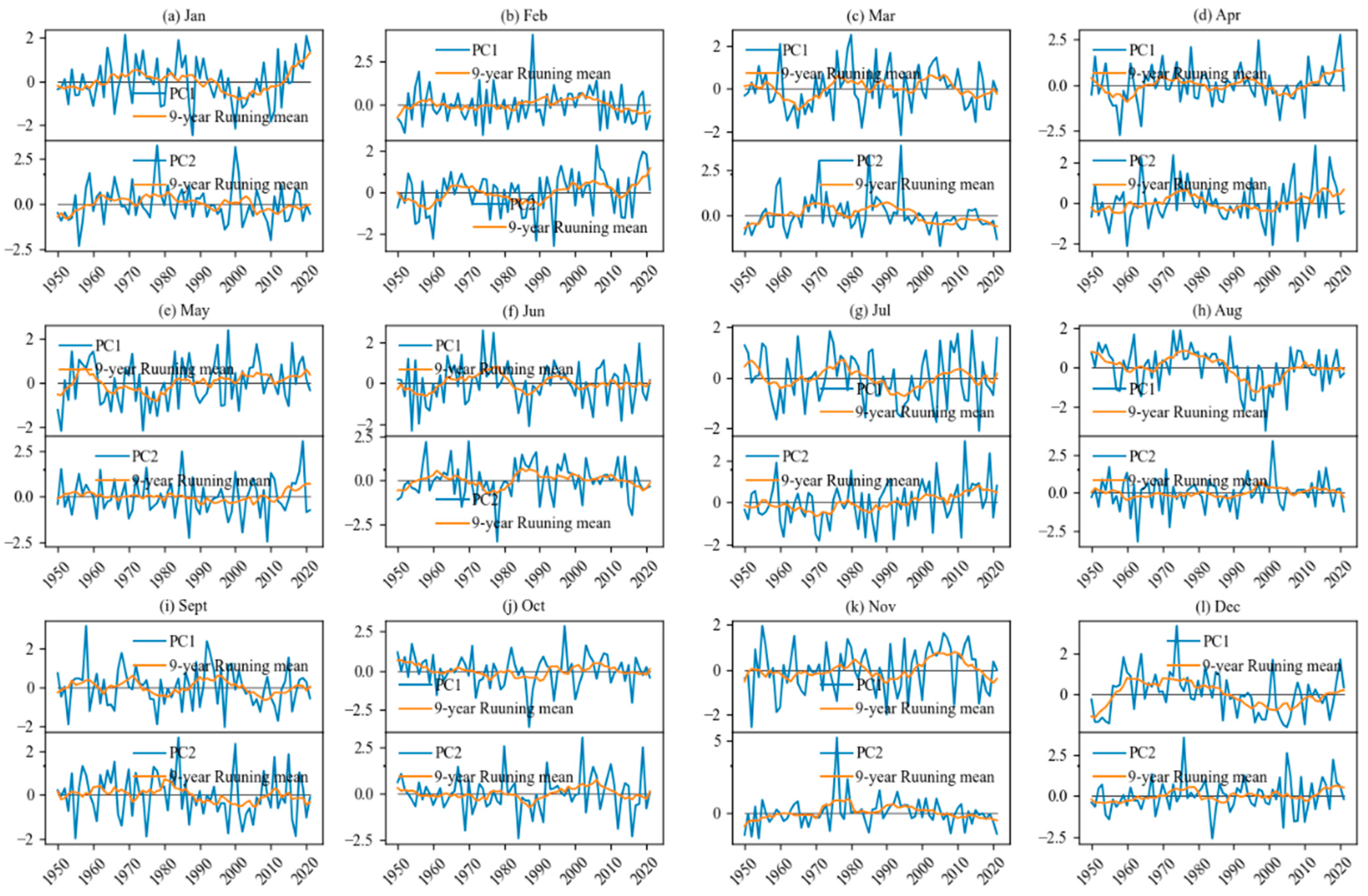
(3)
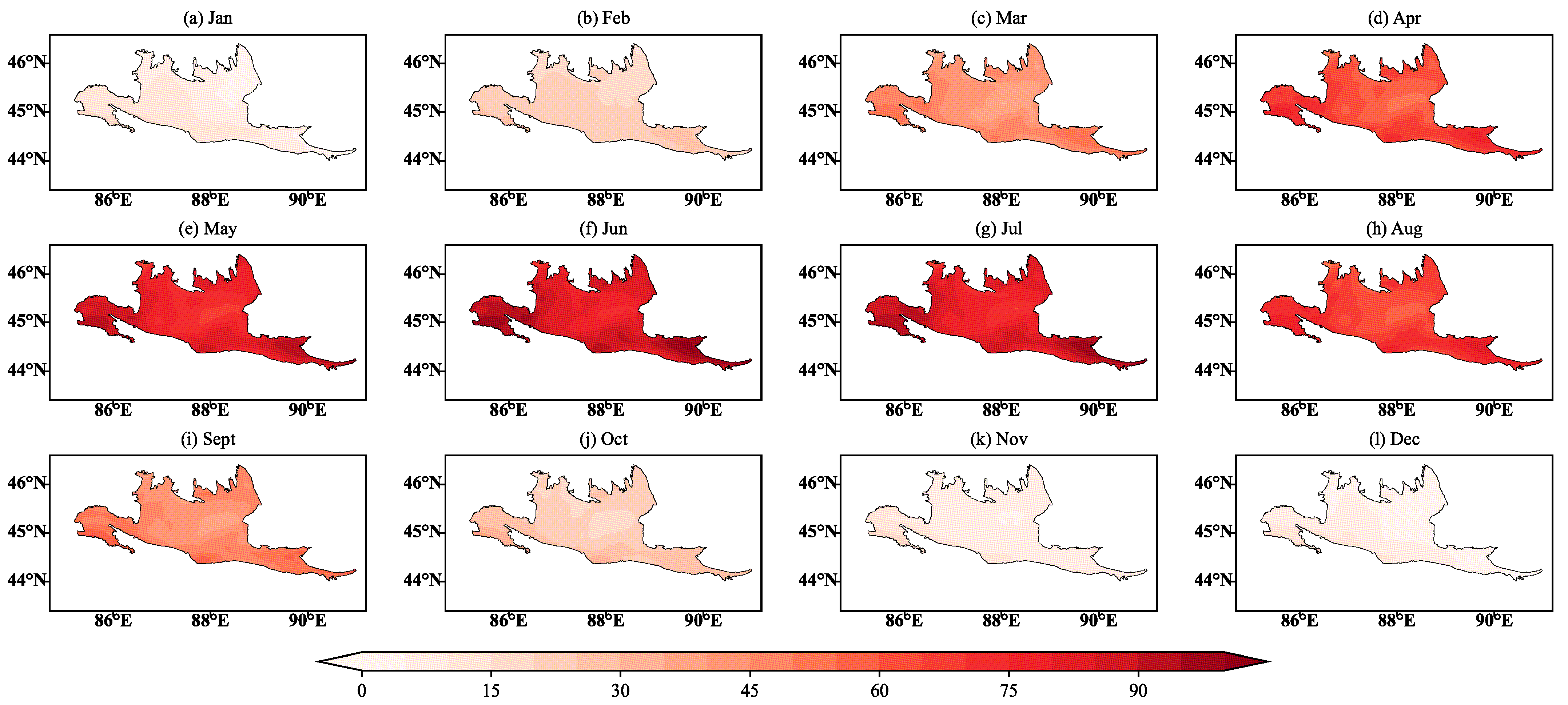
The monthly SHS intensity was lower than 50 W/m2 during the January–March and September–December periods, showing a weak heat source, and was higher than 50 W/m2 during April–August in the Gurbantunggut Desert. The first mode of EOF decomposition can explain the spatio-temporal variation in the monthly SHS intensity in the desert region effectively. On the other hand, EOF1 showed the change characteristics of a consistent strengthening or weakening of the monthly SHS intensity in desert areas. The spatial distribution of EOF2 showed a north–south or east–west polarity variation. The variation characteristics of the time coefficients of the first and second modes of the EOF decomposition from January to December were quite different.
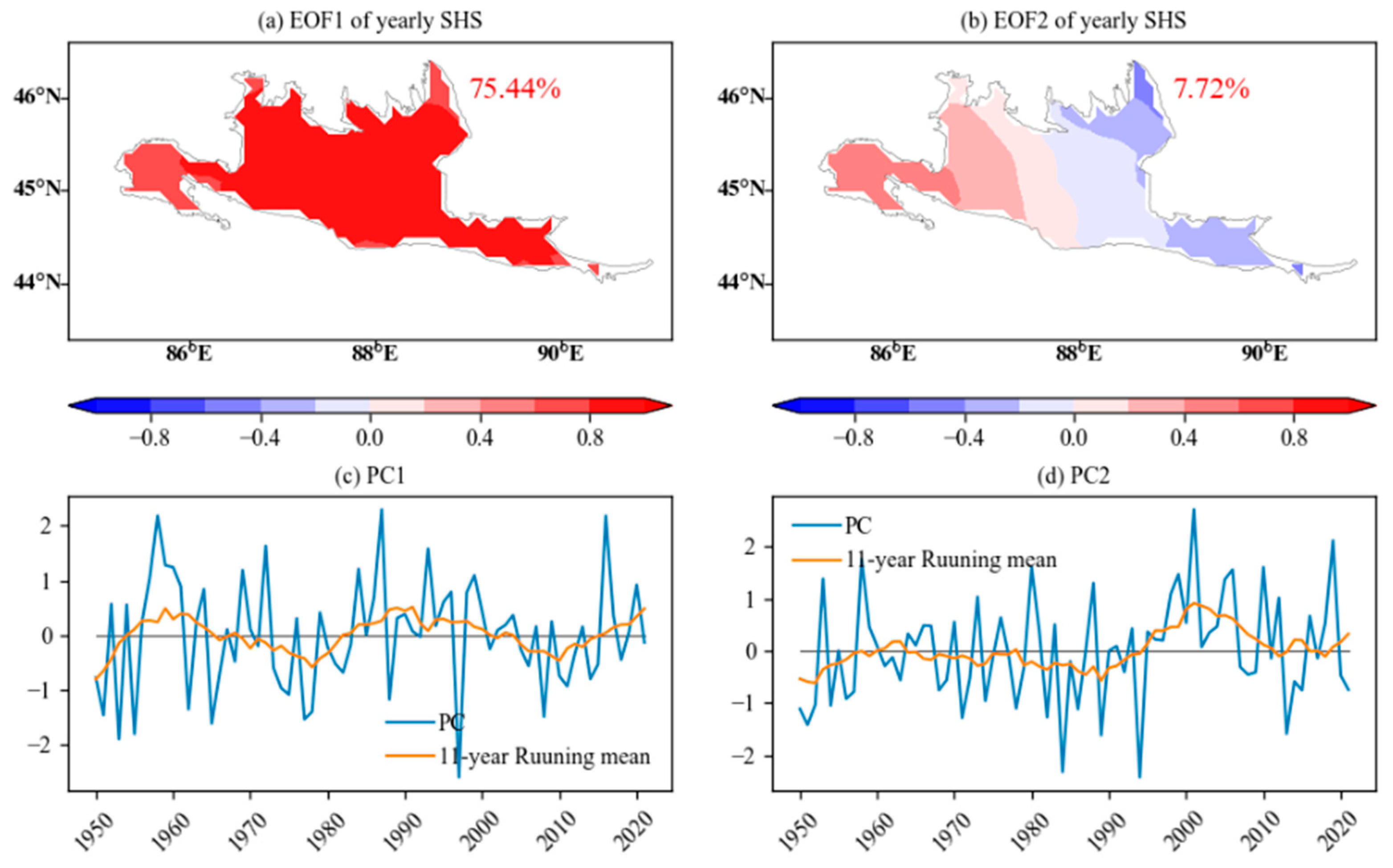
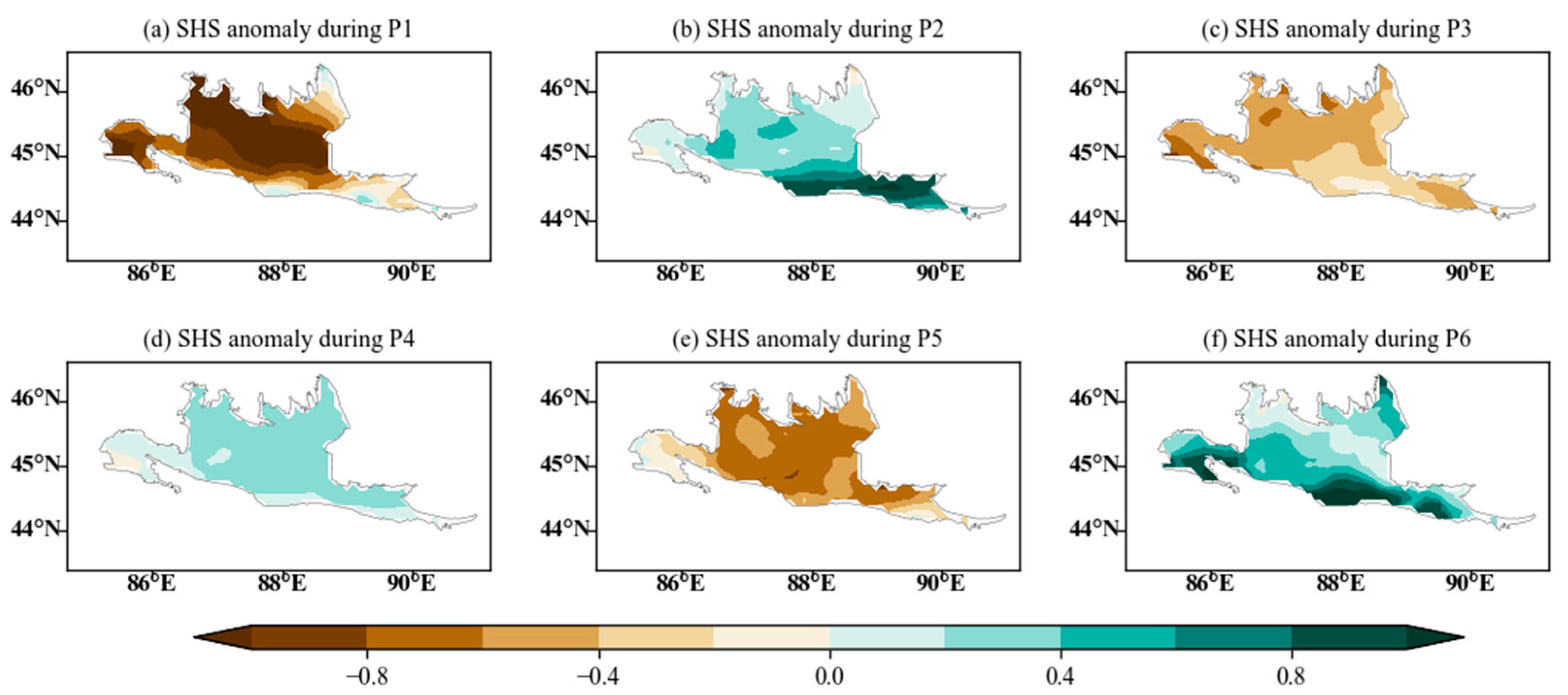
(4)
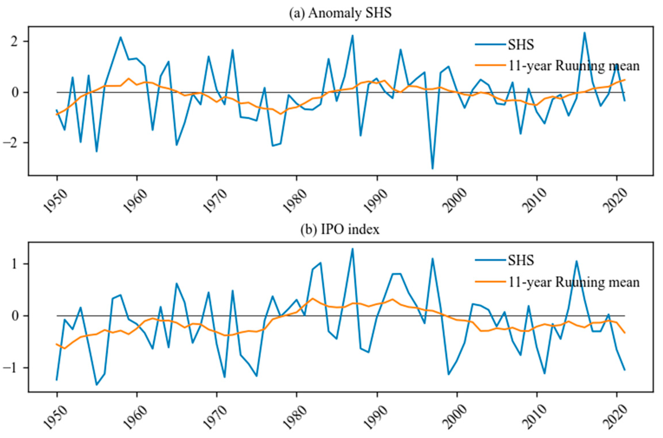
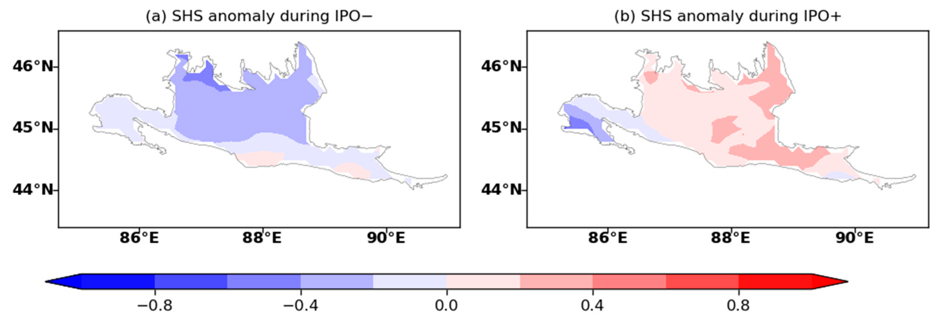
The climatology of the yearly SHS intensity was lower in the central part and higher in the western and eastern parts. The time series of the anomalies in the yearly SHS intensity showed obvious interdecadal variation characteristics. The spatial distribution of the yearly SHS intensity showed negative anomalies at P1, P3 and P5, and positive anomalies at P2, P4 and P6 in the Gurbantunggut Desert. In the negative IPO phase, the yearly SHS anomalies were negative in the Gurbantunggut Desert, while the yearly SHS anomalies were positive in the positive IPO phase in most regions of the Gurbantunggut Desert.

Author Contributions

All authors contributed to the study’s conception and design. Material preparation, data collection and data curation were performed by M.S., C.W. and C.J. The methodology and software were developed by W.H., F.Y., J.L. and J.G. The investigation, visualization, writing—original draft preparation and analysis were performed by A.A., A.M. and Y.W. All authors commented on previous versions of the manuscript. All authors have read and agreed to the published version of the manuscript.

Funding

This research was funded by the Science and Technology Development Fund, Institute of Desert Meteorology, China Meteorological Administration, Urumqi, grant number KJFZ202302; Sandstorm laboratory project, grant number 2023-38; The Central Scientific Research Institute of the Public Basic Scientific Research Business Professional, grant number IDM2021005; The National Natural Science Foundation of China, grant number 42305132 and 41875023; The Science and technology innovation development Foundation of Xinjiang Meteorological Bureau, grant number MS202312; The Innovation Team Project of Xinjiang Meteorological Service, grant number ZD202306.

Data Availability Statement

The datasets used in this study can be supplied by Mamtimin Ali ([email protected]) upon request.

Acknowledgments

Muñoz Sabater, J., (2019) [28] was downloaded from the Copernicus Climate Change Service (C3S) Climate Data Store (2023). We acknowledge the European Centre’s Working Group on Medium-Range Weather Forecasts Reanalysis v5 Land for making their reanalysis available for the analysis of this paper.

Conflicts of Interest

The authors declare no conflict of interest.

References

  1. Yang, T.; Wang, X.; Zhao, C.; Chen, X.; Yu, Z.; Shao, Q.; Xu, C.; Xia, J.; Wang, W. Changes of climate extremes in a typical arid zone: Observations and multimodel ensemble projections. J. Geophys. Res. 2011, 116, D19106. [Google Scholar] [CrossRef]
  2. Xie, Z.; Wang, B. Summer heat sources changes over the Tibetan Plateau in CMIP6 models. Environ. Res. Lett. 2021, 16, 64060. [Google Scholar] [CrossRef]
  3. Yao, J.; Chen, Y.; Guan, X.; Zhao, Y.; Chen, J.; Mao, W. Recent climate and hydrological changes in a mountain–basin system in Xinjiang, China. Earth-Sci. Rev. 2022, 226, 103957. [Google Scholar] [CrossRef]
  4. Mamtimin, A.; Wang, Y.; Sayit, H.; Yang, X.; Yang, F.; Huo, W.; Zhou, C. Seasonal Variations of the Near-Surface Atmospheric Boundary Layer Structure in China’s Gurbantünggüt Desert. Adv. Meteorol. 2020, 2020, 6137237. [Google Scholar] [CrossRef]
  5. Gao, J.; Wang, Y.; Hajigul, S.; Ali, M.; Liu, Y.; Zhao, X.; Yang, X.; Huo, W.; Yang, F.; Zhou, C. Characteristics of surface radiation budget in Gurbantunggut Desert. J. Desert Res. 2021, 41, 47–58. (In Chinese) [Google Scholar]
  6. Huo, W.; Zhi, X.; Yang, F.; Zhou, C.; Wang, Y.; Song, M.; Pan, H.; Ali, M.; He, Q. Energy Budget Difference between Artificial Green Land and Natural Sandy Land in Taklimakan Desert. Desert Oasis Meteorol. 2022, 16, 1–9. (In Chinese) [Google Scholar]
  7. Hua, W.; Fan, G.; Zhou, D.; Ni, C.; Li, X.; Wang, Y.; Liu, Y.; Huang, X. Preliminary analysis of the relationship between vegetation change and surface heat source and precipitation in China over the Qinghai-Tibet Plateau. Sci. China (Ser. D Earth Sci.) 2008, 38, 732–740. (In Chinese) [Google Scholar]
  8. Duan, A.; Xiao, Z.; Wang, Z. Impacts of the Tibetan Plateau winter/spring snow depth and surface heat source on Asian summer monsoon: A review. Chin. J. Atmos. Sci. 2018, 42, 755–766. (In Chinese) [Google Scholar]
  9. Wang, M.; Wang, J.; Chen, D.; Duan, A.; Liu, Y.; Zhou, S.; Guo, D.; Wang, H.; Ju, W. Recent recovery of the boreal spring sensible heating over the Tibetan Plateau will continue in CMIP6 future projections. Environ. Res. Lett. 2019, 14, 124066. [Google Scholar] [CrossRef]
  10. Duan, A.; Li, F.; Wang, M.; Wu, G. Persistent Weakening Trend in the Spring Sensible Heat Source over the Tibetan Plateau and Its Impact on the Asian Summer Monsoon. J. Clim. 2011, 24, 5671–5682. [Google Scholar] [CrossRef]
  11. Wan, Y.; Zhang, Y.; Zhang, J.; Peng, Y. Influence of sensible heat on planetary boundary layer height in East Asia. Plateau Meteorol. 2017, 36, 173–182. (In Chinese) [Google Scholar]
  12. Su, Y.; Lü, S.; Fan, G. The characteristics analysis on the summer atmospheric boundary layer height and surface heat fluxes over the Qinghai-Tibetan Plateau. Plateau Meteorol. 2018, 37, 1470–1485. (In Chinese) [Google Scholar]
  13. Chen, J.; Wu, X.; Yin, Y.; Xiao, H. Characteristics of Heat Sources and Clouds over Eastern China and the Tibetan Plateau in Boreal Summer. J. Clim. 2015, 28, 7279–7296. [Google Scholar] [CrossRef]
  14. Wu, G.; Duan, A.; Liu, Y.; Mao, J.; Ren, R.; Bao, Q.; He, B.; Liu, B.; Hu, W. Tibetan Plateau climate dynamics: Recent research progress and outlook. Natl. Sci. Rev. 2015, 2, 100–116. [Google Scholar] [CrossRef]
  15. Yang, F.; He, Q.; Huang, J.; Mamtimin, A.; Yang, X.; Huo, W.; Zhou, C.; Liu, X.; Wei, W.; Cui, C.; et al. Desert Environment and Climate Observation Network over the Taklimakan Desert. Bull. Am. Meteorol. Soc. 2020, 102, E1172–E1191. [Google Scholar] [CrossRef]
  16. Guo, Y.; Zhang, Y.; Ma, Y.; Ma, N. Surface heat source intensity and surface water/energy balance in Shuanghu, northern Tibetan Plateau. Acta Geogr. Sin. 2014, 69, 983–992. (In Chinese) [Google Scholar]
  17. Chen, Z.; Min, W.; Liu, F. Relationship between Surface Heating Fields over Qinghai-Xizang Plateau and Precipitation in Sichuan Basin during Summer. Meteorological 2003, 29, 9–12. (In Chinese) [Google Scholar]
  18. Yang, X.; Zhu, Y.; Xie, Q.; Ren, X.; Xu, G. Advances in Studies of Pacific Decadal Oscillation. Chin. J. Atmos. Sci. 2004, 28, 979–992. [Google Scholar]
  19. Chan, J.C.L.; Zhou, W. PDO, ENSO and the early summer monsoon rainfall over south China. Geophys. Res. Lett. 2005, 32, 8810. [Google Scholar] [CrossRef]
  20. Duan, W.; Song, L.; Li, Y.; Mao, J. Modulation of PDO on the predictability of the interannual variability of early summer rainfall over south China. J. Geophys. Res.-Atmos. 2013, 118, 13008–13021. [Google Scholar] [CrossRef]
  21. Fu, G.; Viney, N.R.; Charles, S.P.; Liu, J. Long-Term Temporal Variation of Extreme Rainfall Events in Australia: 1910–2006. J. Hydrometeorol. 2010, 11, 950–965. [Google Scholar] [CrossRef]
  22. Xiao, M.; Zhang, Q.; Singh, V.P. Spatiotemporal variations of extreme precipitation regimes during 1961–2010 and possible teleconnections with climate indices across China. Int. J. Climatol. 2017, 37, 468–479. [Google Scholar] [CrossRef]
  23. Dou, J.; Wu, Z.; Li, J. The strengthened relationship between the Yangtze River Valley summer rainfall and the Southern Hemisphere annular mode in recent decades. Clim. Dynam. 2020, 54, 1607–1624. [Google Scholar] [CrossRef]
  24. Aihaiti, A.; Jiang, Z.; Li, Y.; Tao, L.; Zhu, L.; Zhang, J. The global warming and IPO impacts on summer extreme precipitation in China. Clim. Dynam. 2023, 60, 3369–3384. [Google Scholar] [CrossRef]
  25. Zhang, Y.; Wallace, J.M.; Battisti, D.S. ENSO-like Interdecadal Variability: 1900–93. J. Clim. 1997, 10, 1004–1020. [Google Scholar] [CrossRef]
  26. Power, S.; Casey, T.; Folland, C.; Colman, A.; Mehta, V. Inter-decadal modulation of the impact of ENSO on Australia. Clim. Dynam. 1999, 15, 319–324. [Google Scholar] [CrossRef]
  27. Linsley, B.K.; Wu, H.C.; Dassié, E.P.; Schrag, D.P. Decadal changes in South Pacific sea surface temperatures and the relationship to the Pacific decadal oscillation and upper ocean heat content. Geophys. Res. Lett. 2015, 42, 2358–2366. [Google Scholar] [CrossRef]
  28. Muñoz Sabater, J. ERA5-LAND Monthly Averaged Data from 1950 to Present. Copernicus Climate Change Service (C3S) Climate Data Store (CDS). 2019. Available online: https://cds.climate.copernicus.eu/cdsapp#!/dataset/10.24381/cds.68d2bb30?tab=overview (accessed on 8 January 2023).
  29. Henley, B.J.; Gergis, J.; Karoly, D.J.; Power, S.; Kennedy, J.; Folland, C.K.; Naturvetenskapliga, F.; Faculty, O.S.; Göteborgs, U.; Institutionen, F.G.; et al. Tripole Index for the Interdecadal Pacific Oscillation. Clim. Dynam. 2015, 45, 3077–3090. [Google Scholar] [CrossRef]
  30. Wilson, K.; Goldstein, A.; Falge, E.; Aubinet, M.; Baldocchi, D.; Berbigier, P.; Bernhofer, C.; Ceulemans, R.; Dolmanh, H.; Field, C.; et al. Energy balance closure at FLUXNET sites. Agr. Forest Meteorol. 2002, 113, 223–243. [Google Scholar] [CrossRef]
  31. Zhang, F.; Liu, A.; Li, Y.; Zhao, L. Primary Study on Surface Heating Field and Biomass in Alpine Kobresia Meadow in the Qinghai-Tibetan Plateau. Chin. J. Agrometeorol. 2007, 28, 144–148. (In Chinese) [Google Scholar]
  32. Hersbach, H.; Bell, B.; Berrisford, P.; Hirahara, S.; Horányi, A.; Muñoz Sabater, J.; Nicolas, J.; Peubey, C.; Radu, R.; Schepers, D.; et al. The ERA5 global reanalysis. Q. J. Roy. Meteor. Soc. 2020, 146, 1999–2049. [Google Scholar] [CrossRef]
  33. Sheather, S.J.; Jones, M.C. A Reliable Data-Based Bandwidth Selection Method for Kernel Density Estimation. J. R. Stat. Society. Ser. B Methodol. 1991, 53, 683–690. [Google Scholar] [CrossRef]
  34. Coles, S. An Introduction to Statistical Modeling of Extreme Values; Springer: London, UK, 2001. [Google Scholar]
  35. Lane, D. Introduction to Statistics; Rice University: Houston, TX, USA, 2003. [Google Scholar]
  36. Wei, F. The Current Statistical Climatic Diagnosis and Forecasting Technolog; Meteorological Press: Beijing, China, 2007. (In Chinese) [Google Scholar]
  37. Li, Y.; Smith, I. A Statistical Downscaling Model for Southern Australia Winter Rainfall. J. Clim. 2009, 22, 1142–1158. [Google Scholar] [CrossRef]
  38. Lai, X.; Fan, G.; Hua, W.; Ding, X. Progress in the Study of Influence of the Qinghai-Xizang Plateau Land Atmosphere Interaction on East Asia Regional Climate. Plateau Meteorol. 2021, 40, 1263–1277. (In Chinese) [Google Scholar]
  39. Gao, Q.; Weng, D. Climatological Characteristics of Ground Heat Sources over China. J. Nanjing Inst. Meteorol. 1995, 18, 543–547. (In Chinese) [Google Scholar]
  40. Duan, A.; Wang, M.; Lei, Y.; Cui, Y. Trends in Summer Rainfall over China Associated with the Tibetan Plateau Sensible Heat Source during 1980–2008. J. Clim. 2013, 26, 261–275. [Google Scholar] [CrossRef]
  41. Li, H. Land Surface Energy Exchange over Mainland China and Preliminary Analysis of Its Responses to Large-Scale Climate Change. Ph.D. Thesis, Nanjing University, Nanjing, China, 2015. (In Chinese). [Google Scholar]
  42. Du, Y. The Interaction between Land Surface and Atmosphe Ric Boundary Layer in Northwest Region and Its Response to the Summer Monsoon. Master’s Thesis, Lanzhou University, Lanzhou, China, 2018. (In Chinese). [Google Scholar]
  43. Aguedjou, H.M.A.; Chaigneau, A.; Dadou, I.; Morel, Y.; Baloïtcha, E.; Da-Allada, C.Y. Imprint of Mesoscale Eddies on Air-Sea Interaction in the Tropical Atlantic Ocean. Remote Sens. 2023, 15, 3087. [Google Scholar] [CrossRef]
Figure 1. (a) The KLML station and (b) terrain of the study area, with the location of the Gurbantunggut Desert (red area) and KLML station (red triangle). The dotted lines represent the boundaries of northern, eastern and southern Xinjiang.
Remotesensing 15 05731 g001
Figure 2. Hourly variation in the surface heat source in each month from 2013 to 2021 at the KLML station (local time).
Remotesensing 15 05731 g002
Figure 3. Variation in the daily, daytime and night means of the SHS in 2013–2021. All curves represent the 9-day running means of the SHS.
Remotesensing 15 05731 g003
Figure 4. (a) The yearly and (b) monthly mean changes in the SHS at the KLML station in 2013–2021.
Remotesensing 15 05731 g004
Figure 5. The (a) QQ plot, (b) PDF curve, (c) scatter plot and (d) time series of the monthly SHS intensity of the observation and ERA5-Land reanalysis during the 2013–2021 period. The red solid line indicates 1-1 line in (a).
Remotesensing 15 05731 g005
Figure 6. The average spatial distribution of (al) the January–December SHS intensity in the Gurbantunggut Desert during the 1950–2021 period.
Remotesensing 15 05731 g006
Figure 7. Spatial distribution of the first two modes of the EOF decomposition of the SHS intensity during (al) January–December in the Gurbantunggut Desert.
Remotesensing 15 05731 g007
Figure 8. Time coefficients of the first two modes of the EOF decomposition of the SHS intensity during (al) January–December in the Gurbantunggut Desert. The blue and orange solid lines represent the original sequence and the 11-year running mean, respectively.
Remotesensing 15 05731 g008
Figure 9. The (a) climatology, (b) trend and (c) time series of the anomalies of the yearly SHS intensity in the Gurbantunggut Desert during the 1950–2021 period. The anomalies in the SHS intensity were relative to the base period, i.e., 1981–2010. P1–P6 in (c) represent the SHS intensity positive and negative anomaly periods. P1–P6 refer to 1950–1954, 1955–1963, 1964–1982, 1983–2003, 2004–2015 and 2016–2021, respectively. The blue and orange solid lines in (c) represent the original sequence and the 11-year running mean, respectively.
Remotesensing 15 05731 g009
Figure 10. The (a,b) spatial distributions and (c,d) time coefficients of the first two modes of the EOF decomposition of the yearly SHS intensity in the Gurbantunggut Desert during 1950–2021. The blue and orange solid lines in (c,d) represent the original sequence and the 11-year running mean, respectively.
Remotesensing 15 05731 g010
Figure 11. The spatial distribution of the yearly SHS intensity anomalies at (af) P1–P6, respectively. The anomalies in the SHS intensity are relative to the base period, i.e., 1981–2010.
Remotesensing 15 05731 g011
Figure 12. The time series of (a) the SHS intensity anomalies and (b) IPO index during the 1950–2021 period. The anomalies of the SHS were relative to the base period, i.e., 1981–2010. The blue and orange solid lines represent the original sequence and the 11-year running mean, respectively.
Remotesensing 15 05731 g012
Figure 13. The spatial distribution of the yearly SHS intensity anomalies during the IPO (a) negative and (b) positive phases, respectively. The anomalies in the SHS intensity were relative to the base period, i.e., 1981–2010.
Remotesensing 15 05731 g013
Figure 14. The spatial distribution characteristics of precipitation anomalies in the IPO (a) negative and (b) positive phases in northern Xinjiang.
Remotesensing 15 05731 g014
Table 1. The RMSE, MAE, interannual variations (i.e., regression coefficients), R2 and correlation coefficients of the monthly SHS intensity between the observation and the ERA5-Land reanalysis at the KLML station during the 2013–2021 period.
RMSEMAEInterannual VariationsR2Corr.
ObservationERA5-Land
9.56 W/m28.32 W/m20.016 W/m2−0.013 W/m20.900.96
Table 2. The anomaly periods of the yearly SHS intensity during the 1950–2021 period in the Gurbantunggut Desert.
PeriodPeriodSHS Anomaly
P11950–1954negative
P21955–1963positive
P31964–1982negative
P41983–2003positive
P52004–2015negative
P62016–2021positive
Disclaimer/Publisher’s Note: The statements, opinions and data contained in all publications are solely those of the individual author(s) and contributor(s) and not of MDPI and/or the editor(s). MDPI and/or the editor(s) disclaim responsibility for any injury to people or property resulting from any ideas, methods, instructions or products referred to in the content.

