Improving Colored Dissolved Organic Matter (CDOM) Retrievals by Sentinel2-MSI Data through a Total Suspended Matter (TSM)-Driven Classification: The Case of Pertusillo Lake (Southern Italy)

Abstract

Colored dissolved organic matter (CDOM) is a significant constituent of aquatic systems and biogeochemical cycles. Satellite CDOM retrievals are challenging in inland waters, due to overlapped absorption properties of bio-optical parameters, like Total Suspended Matter (TSM). In this framework, we defined an accurate CDOM model using Sentinel2-MSI (S2-MSI) data in Pertusillo Lake (Southern Italy) adopting a classification scheme based on satellite TSM data. Empirical relationships were established between the CDOM absorption coefficient, a_CDOM (440), and reflectance band ratios using ground-based measurements. The Green-to-Red (B3/B4 and B3/B5) and Red-to-Blue (B4/B2 and B5/B2) band ratios showed good relationships (R² ≥ 0.75), which were further improved according to sub-region division (R² up to 0.93). The best accuracy of B3/B4 in the match-ups between S2-MSI-derived and in situ band ratios proved the exportability on S2-MSI data of two B3/B4-based a_CDOM (440) models, namely the fixed (for the whole PL) and the switching one (according to sub-region division). Although they both exhibited good agreements in a_CDOM (440) retrievals (R² ≥ 0.69), the switching model showed the highest accuracy (RMSE of 0.0155 m⁻¹). Finally, the identification of areas exposed to different TSM patterns can assist with refining the calibration/validation procedures to achieve more accurate a_CDOM (440) retrievals.

1. Introduction

Colored dissolved organic matter (CDOM) is the photoactive constituent of dissolved organic carbon (DOC), which is the most prominent organic carbon pool in water environments [1]. CDOM is crucial in aquatic ecological processes as it reduces light penetration which impacts net primary production and the thermal properties of water ecosystems [2,3,4,5]. Furthermore, CDOM is a key parameter for inland water quality as its influence on pH, alkalinity, and the formation of potentially toxic metal complexes affects drinking water safety [6,7]. Assessing the accuracy of CDOM retrievals and understanding its spatiotemporal distribution is crucial to studying the carbon cycle of aquatic ecosystems and managing their water quality status as well [8].

The joint exploitation of field spectroscopy and satellite data has proved useful in retrieving CDOM estimates in estuaries and inland waters [9,10]. In the last three decades, most of the CDOM retrieval algorithms relied on empirical [11,12,13,14] or semi-analytical [15,16,17,18] models. More recently, some methods based on machine learning (ML) approaches [19,20,21] have been proposed showing encouraging results at the global scale [21]. However, the ML models usually rely on intricate structures of input variables and their development requires large in situ training databases (i.e., hyperspectral radiometric measurements and co-located water quality data) which are difficult to obtain in real-world scenarios [22]. Furthermore, the need to consider homogenous data (e.g., same spectral, spatial, and temporal information) for transferability of already trained ML algorithms limits their exportability over space and time [22]. Conversely, the semi-analytical algorithms are more suitable to be regionally optimized as they rely on a transparent and modular structure [23], which allows for a customization of the empirical relationships on which are based [24]. For instance, the Quasi-Anlytical Algorithm (QAA) has been widely implemented in operational chains [25,26] and/or modified to optimize its suitability for CDOM retrievals in complex riverine and estuarine waters [27,28]. Although strong physical bases characterize such semi-analytical models, their implementation in different inland water types requires knowledge of site-specific bio-optical parameters (e.g., particulate backscattering, b_bp (λ)) or optimization approaches (i.e., radiative transfer models) that can increase CDOM retrieval uncertainties [8]. The empirical algorithms are based on a few basic relationships between apparent and inherent optical water properties and, thus are easier to be implemented compared with the semi-analytical ones. On the other hand, they are particularly sensitive to changes in boundary conditions [29]. For this reason, most of the regional studies for CDOM estimates in freshwaters used empirical methods (e.g., regression) based on remote sensing reflectance (Rrs) and CDOM absorption indices [30].

Most such algorithms [14,31,32] require input Rrs at different wavelengths within the visible spectral domain (≈400–700 nm) combined in different band ratios [33]. Such a spectral domain is generally available on the main land-oriented satellite sensors (e.g., Landsat Thematic Mapper-TM, Enhanced Thematic Mapper Plus-ETM+, and EO-1 Advanced Land Imager-ALI) or ocean color spectrometers (e.g., Sea-viewing Wide Field-of-view Sensor-SeaWiFS, Moderate-Resolution Imaging Spectroradiometer-MODIS, Visible Infrared Imaging Radiometer Suite–VIIRS, and Medium-Resolution Imaging Spectrometer-MERIS), which are no longer available and are unsuitable for most inland water bodies because of their coarse spatial resolutions [34]. To overcome these limitations, the most recent Earth Observation (EO) sensors, such as the MultiSpectral Instrument (MSI) on Sentinel-2A/B (S2), offer many advantages for lake remote sensing thanks to a high revisiting time (up to 5 days) and 10–60 m spatial resolution together with a suitable spectral capability [35].

Several studies have demonstrated the S2-MSI suitability for CDOM estimation in inland waters, by exploiting especially the Green (e.g., B3) to Red (e.g., B4, B5, B6, and B7) band ratios [36]. Toming et al. [37] and Al-Kharusi et al. [33] used the B3 (560 nm central wavelength) to B4 (665 nm central wavelength) ratio for estimating CDOM absorption (a_CDOM) by S2-MSI data in several lakes of Estonia and Sweden, respectively. Xu et al. [8] and Shang et al. [30] have profitably adopted the B5 (665 nm central wavelength) to B2 (492 nm central wavelength) ratio to develop empirical CDOM models and characterize its spatial dynamics in Chinese water reservoirs. The above studies have corroborated the need to calibrate CDOM models at regional and locale scales by accounting for differences in water bio-chemical properties across geographical regions [30].

Pertusillo Lake (hereinafter PL), situated in the Basilicata region (Southern Italy), is considered a sensitive test site for the Italian Ministry of the Environment, because of its environmental relevance in terms of ongoing anthropogenic pressures (e.g., proximity to the largest onshore oil field in Europe [38]) and ecosystem bio-optical complexity [39]. Furthermore, environmental forcings, such as water-level fluctuations and river discharges usually cause erosion, sediment resuspension, and changes in nutrient inputs, thus determining a high variability of the in-water bio-optical components [40]. PL has been never studied up to now in terms of CDOM retrievals, but only to detect a potentially harmful algal bloom using remote sensing data [39] or to assess the multi-temporal total suspended matter (TSM) variability by merging S2-MSI and Landsat 8 (L8)-Operational Land Imager (OLI) records [40]. The latter study showed how PL can be divided into two areas with different TSM spatial patterns probably due to eastward changes in hydrological (i.e., inflowing rivers) and bathymetric characteristics.

In this scenario, it is worth developing and validating CDOM models by adopting a methodological approach that considers the spatial heterogeneity of water ecosystems induced by hydrological forcing and topographic features and highlighted by the spatial variability of other in-water constituents (e.g., TSM). In this study, we aim to define an accurate CDOM retrieval model using S2-MSI data through the adoption of a previously achieved classification scheme based on satellite TSM data [40]. Finally, the three-fold goals of this work were to: (a) assess the performance of two literature a_CDOM (440) algorithms, namely an empirical [14] and a semi-analytical one [27] when ported on PL; (b) define a customized version of S2-MSI a_CDOM (440) model by using in situ radiometric data and a_CDOM (440) measurements; (c) maximize the accuracy of such a PL-tuned algorithm via a switchable scheme based on a pixel membership to the two sub-regions identified using the TSM-driven classification.

2. Materials and Methods

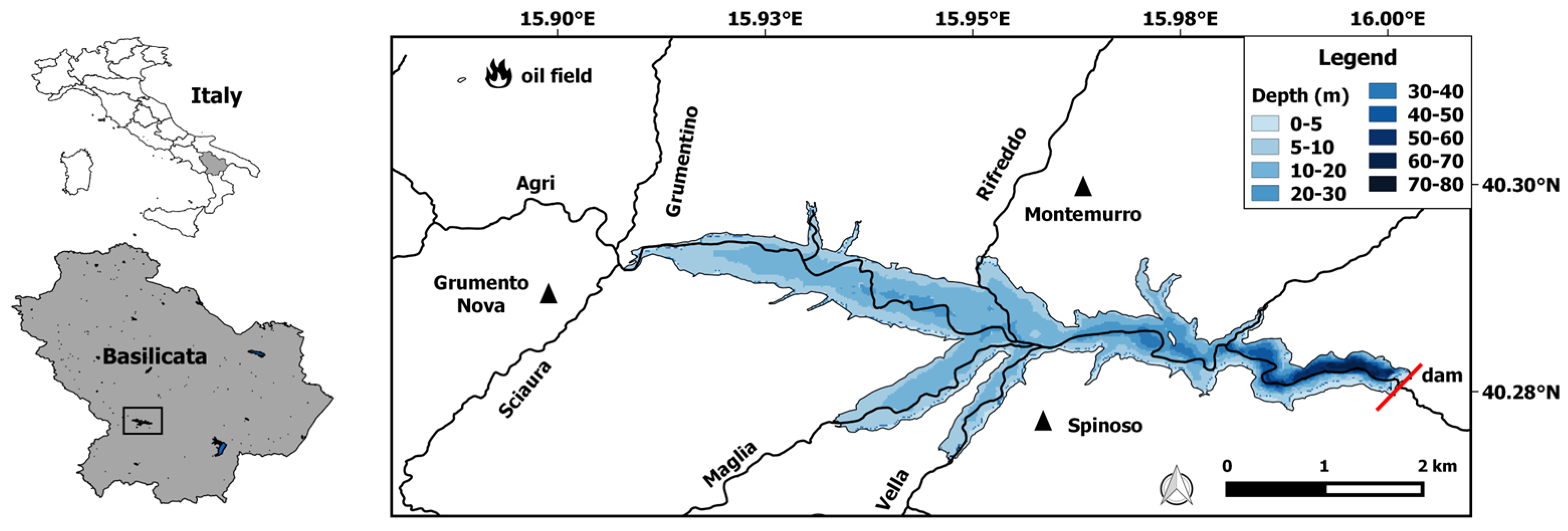
2.1. Study Site

The PL is an artificial freshwater reservoir situated in the high Agri Valley of the Basilicata region (Southern Italy) (Figure 1). The PL, constructed during the 1957–1963 years by damming the Agri River, covers a surface of 7.5 km² with approximately 80 m and 155 × 10⁶ m³ maximum depth and volume, respectively [40]. It serves the Apulian Aqueduct in providing drinking water to 3.5 million people as well as for irrigation and hydroelectric energy production [41].

The PL shows a well-defined water level variability, mainly because of seasonal rainfall and discharge of rivers, such as the Agri River that flows eastward along the lake basin [42]. Furthermore, the dam-induced hydrological regime and the torrential discharges of other minor tributaries (i.e., Rifreddo, Grumentino, Maglia, Vella, and Sciaura rivers) influence the PL net volume fluctuations and contribute to drain areas with different sediment types at several lake locations [40].

PL Sub-Region Division: The ISODATA Classification

The recent work by Ciancia et al. [40] allowed for the identification of two sub-regions characterized by different TSM spatial patterns. In particular, using a multi-temporal analysis of TSM monthly maps obtained by S2-MSI and L8-OLI merged data, Ciancia et al. [40] carried out a classification analysis to discriminate lake areas showing similar TSM spatial patterns within climatology. The ISODATA (Iterative Self-Organizing Data Analysis technique) unsupervised classification [43] was applied by using 5-year (2014–2018) TSM climatological monthly means as “input spectral bands” and setting user-defined threshold parameters (i.e., the maximum number of iterations and change threshold).

Figure 2 shows the PL sub-region division after implementing the ISODATA unsupervised classification scheme on the MSI-OLI merged TSM dataset for the 5-year period, as discussed in Ciancia et al. [40].

Considering the TSM climatological variability, two distinct sub-areas (i.e., the West and East areas) have been identified, showing different suspended sediment concentrations, hydrological forcing levels, and topography (i.e., bathymetry) [40]. The PL’s western region is mainly affected by water level fluctuations and consequent deposition and erosion phenomena due to shallow waters and multiple longitudinal and lateral deltas. Conversely, PL’s eastern side is characterized by smaller loads of suspended particles probably as no major rivers are inflowing there [40].

2.2. In Situ Data Acquisition

During the ‘Smart Basilicata’ project [44], six measurement campaigns were planned and carried out to investigate the spatiotemporal variability of some bio-optical constituents (e.g., TSM and a_CDOM (440)) over the lake. Sub-surface water samples and radiometric parameters were acquired at planned stations (Figure 2) in the period from May 2017 to May 2018. Information regarding the in situ measurement campaigns (with distinction between the two different subset) is listed in

Table 1. Sampling campaigns and data used. Note that Rrs(λ) data were not acquired in September 2017 (19th).

Measurement Campaigns	Number of Samples		In Situ Measurements
	West Subset	East Subset
May 2017 (10th, 26th)	12	8	TSM, aCDOM (440), Rrs(λ)
June 2017 (14th, 15th)	12	8	TSM, aCDOM (440), Rrs(λ)
September 2017 (19th)	5	4	TSM, aCDOM (440)
October 2017 (12th)	4	4	TSM, aCDOM (440), Rrs(λ)
November 2017 (21st)	4	4	TSM, aCDOM (440), Rrs(λ)
May 2018 (17th)	6	4	TSM, aCDOM (440), Rrs(λ)

.

Sub-surface (i.e., 0–1 m depth) water samples were collected by Niskin bottles for subsequent TSM measurements and analyses of CDOM absorption spectra.

2.2.1. The a_CDOM (440) and TSM Measurements

For the TSM estimates, we adopted standard gravimetrical protocols [45,46]. After collecting 500–1000 mL of water samples, a filtering procedure was applied through 0.7 µm pre-weighed GF/F glass fiber filters. Moreover, the samples were rinsed with distilled water and dried at 100 °C. Finally, they were re-weighed by an electronic balance (Mettler Toledo AG245) with a 0.1 mg detection limit [40].

For the CDOM absorption measurements, 200 mL of water per station was filtered through previously washed sterile 0.2 µm filters (Whatman GD/X). Afterward, amber glass bottles, previously acid-soaked (10% HCl) and 3 times washed with Milli-Q water, were used to stock the filtered water samples. Finally, the filtered and collected water samples were maintained at a 4 °C constant temperature until the absorption measurements (within a maximum of four weeks). CDOM absorption spectra were measured in a 10 cm quartz cuvette between 250 and 750 nm spectral range through a dual beam UV-VIS spectrophotometer (SHIMADZU 2600 Series) [47]. The CDOM absorption coefficient, a_CDOM (λ), was obtained using Equation (1):

$${\mathrm{a}}_{\mathrm{C}\mathrm{D}\mathrm{O}\mathrm{M}}\left(\lambda \right)=2.303\ast A_{\left(\lambda \right)}/\mathrm{L},$$

(1)

where L is the cuvette length (m), A_(λ) the measured optical density and a_CDOM (λ) represents the CDOM concentration at the computation wavelength λ. The CDOM spectral slope (S_CDOM) was computed by using an exponential function as reported in Equation (2) [48]:

$${\mathrm{a}}_{\mathrm{C}\mathrm{D}\mathrm{O}\mathrm{M}}\left(\lambda \right)={\mathrm{a}}_{\mathrm{C}\mathrm{D}\mathrm{O}\mathrm{M}}\left({\lambda }_0\right)\ast \mathrm{e}\mathrm{x}\mathrm{p}\left[-{\mathrm{S}}_{\mathrm{C}\mathrm{D}\mathrm{O}\mathrm{M}}(\lambda -{\lambda }_0)\right],$$

(2)

where S_CDOM is the fitted parameter for the exponential decay of a_CDOM(λ) with increasing wavelength λ respect to λ₀, that is the reference wavelength at 440 nm. In this study, we analyzed the spectral slope within the 350–500 nm wavelength range (i.e., S_CDOM (350–500)) to ensure a sufficiently high signal-to-noise ratio [49].

Table 2. Descriptive statistics of a_CDOM (440) derived from the six measurement campaigns.

Parameter	Values	PL	West Subset	East Subset
aCDOM (440) (m−1)	min	0.1277	0.1414	0.1277
	max	0.4145	0.4145	0.2533
	mean	0.2252	0.2450	0.1980
	stdv	0.0678	0.0756	0.0396
TSM (g/m3)	min	0.6	1	0.6
	max	7	7	2.6
	mean	2.0829	2.3679	1.7029
	stdv	1.1270	1.3296	0.6252

summarizes the descriptive statistics of a_CDOM (440) and TSM derived from the six measurement campaigns and related to the whole area, the West and East subset, respectively.

The a_CDOM (440) values range from 0.1277 to 0.4145 m⁻¹ with higher mean values in the West subset than the East one while S_CDOM (350–500 nm) records an averaged value of 0.0168 nm⁻¹ with negligible differences between sub-regions. The TSM estimations are within 0.6–7 g/m³ and spatially differ with higher mean values in the West subset than the East one as for a_CDOM (440).

2.2.2. Radiometric Rrs(λ) Measurements

Simultaneously to water samples, the above-water radiometric data were acquired and processed according to standard protocols [50]. By using a portable field spectroradiometer (i.e., Field Spec FR PRO spectrometer Analytical Spectral Devices—ASD), in situ radiance measurements were acquired from a boat (at about 1.5 m height above the water surface) within 10:00 to 15:00 only in absence of clouds and with low wind velocity conditions (maximum 5 m/s). To avoid direct sunlight and boat shadows, radiance measurements were acquired positioning the probe at 45° zenith angle and 90 or 180° azimuth angle [50]. Water leaving radiances were measured, pointing the radiometer downwards to the lake, while sky radiances rotating it upwards and retaining the same zenithal and azimuthal angles. Then, was normalized via measurements through a gray (30% albedo) panel (standard Spectralon, Labsphere, NH, USA), assuming that it has a near-Lambertian behavior, to calculate the downwelling spectral irradiance on the water surface (Es(λ)). Furthermore, to reduce potential sources of noise in signal acquisition at least 5 spectra were acquired and averaged for each measurement station.

Finally, it was possible to derive the remote sensing reflectance Rrs(λ) (sr⁻¹), namely the ratio of water leaving radiance L_w(θ,φ,λ) (Wm⁻²nm⁻¹sr⁻¹) to downwelling spectral irradiance Es(λ) (Wm⁻²nm⁻¹) [51]:

$${\mathrm{R}}_{\mathrm{r}\mathrm{s}}\left(\lambda \right)=\frac{{\mathrm{L}}_{\mathrm{w}}(\mathrm{ϴ},\mathsf{\Phi },\lambda )}{{\mathrm{E}}_{\mathrm{s}}(\lambda )},$$

(3)

All the acquired spectra were analyzed using the ViewSpec Pro software 6.0 (ASD Inc., Boulder, CO, USA [52]).

2.3. Satellite Data Acquisition and Processing

S2-MSI data were used in this work to develop a PL-tuned version of a_CDOM (440) model. MSI is a multi-spectral instrument acquiring the emitted/reflected Earth radiance in 13 spectral bands with 10–60 m spatial resolution in the whole electromagnetic spectrum (i.e., 440–2202 nm) and 10–20 m within the visible domain of interest (i.e., 492–704 nm) for a_CDOM (440) modeling (

Table 3. Central wavelength (nm) and spatial resolution (m) of the S2-MSI bands used in this study.

S2-MSI Spectral Bands	Blue2 B2	Green B3	Red1 B4	Red2 B5	SWIR1 B11
central wavelength (nm)	492	560	665	704	1614
spatial resolution (m)	10	10	10	20	20

).

Level-1 S2 MSI images (MSI-L1C) were downloaded from the ESA’s Scientific Data Hub [53]. All the MSI-L1C data falling within the in-situ sampling dates were processed.

MSI-L1C data were re-sampled at 20 m and processed to generate L2 products (i.e., Rrs(λ)) via the ACOLITE software (version 20220222) [54]. To derive atmospherically corrected L2 data, the multi-band “dark spectrum fitting” (DSF) method has been used since it was properly designed for aquatic remote sensing applications, especially in coastal and inland waters [55]. Furthermore, a sun glint correction to the MSI data was applied by adopting a SWIR-based threshold (pixels with sea surface reflectance at 1600 nm ≥ 0.11 were excluded) that is user-tunable within the ACOLITE tool [55].

Afterward, a fixed threshold (at 1600 nm) was applied to identify land/cloud pixels to be excluded from further processing. The latter procedure allowed for the MSI-L2 Rrs(λ) retrievals as input variables for the a_CDOM (440) models.

2.4. CDOM Estimation Algorithms

Before developing a new customized a_CDOM (440) model, we first assessed the accuracy of two literature algorithms, namely an empirical style [14] and a semi-analytical one [27]. Among the empirical models viable in literature and tested by recent works [21,56], we selected the Ficek et al. [14] algorithm owing to its superior statistical indicators and error metrics within the satellite-in situ match-ups [56]. Such an algorithm relies on a band ratio of Green to Red, where a_CDOM (440) can be defined as follows:

$${\mathrm{a}}_{\mathrm{C}\mathrm{D}\mathrm{O}\mathrm{M}}\left(440\right)=3.65\ast {\left(\frac{Rrs\left(570\right)}{Rrs\left(655\right)}\right)}^{-1.93},$$

(4)

Concerning the semi-analytical algorithms, we evaluated the QAA-CDOM [27] considering its proved suitability also for waters with low CDOM values (a_CDOM (440) < 1 m⁻¹) [27]. The QAA-CDOM scheme was developed from the original QAA [15,16], namely a sequential step-based scheme characterized by empirical (between Rrs and Inherent Optical Properites-IOPs) and analytical relationships.

Steps of the QAA-CDOM (version 5–V5) procedure can be found in Appendix A. For brevity, a_CDOM (440) can be estimated from the reported IOPs as follows:

$${\mathrm{a}}_{\mathrm{p}}\left(440\right)=0.63\ast {\mathrm{b}}_{\mathrm{b}\mathrm{p}}^{0.88},$$

(5)

$${\mathrm{a}}_{\mathrm{C}\mathrm{D}\mathrm{O}\mathrm{M}}\left(440\right)=\mathrm{a}\left(440\right)-{\mathrm{a}}_{\mathrm{w}}\left(440\right)-{\mathrm{a}}_{\mathrm{p}}\left(440\right),$$

(6)

where a, a_p, and a_w are total, particulate, and pure water absorption, respectively, and b_bp is the particulate backscattering. The above-mentioned a_CDOM (440) algorithms were implemented on the in situ Rrs(λ) data considering the availability of a large enough dataset of measurements over the investigated area.

2.5. Model Calibration and Validation

The development of a PL-tuned a_CDOM (440) model on S2-MSI data relies on calibration/validation (cal/val) steps. Before calibration, a preliminary procedure was required to simulate the S2-MSI bands from the in-situ measured Rrs(λ) spectra. According to the spectral response functions of the S2-MSI bands [57], SRF(λ), we applied the following formula [58]:

$${\mathrm{R}\mathrm{r}\mathrm{s}}_{\mathrm{e}\left(\mathrm{i}\right)}=\frac{{\int }_{\lambda min}^{\lambda max}SRF\left(\lambda \right)Rrs\left(\lambda \right)d\lambda }{{\int }_{\lambda min}^{\lambda max}SRF\left(\lambda \right)d\lambda },$$

(7)

where Rrs_e(i) is the equivalent remote sensing reflectance for _i-band of S2-MSI while Rrs(λ) is the in situ measured one; λ_min and λ_max are the lowest and highest wavelengths within the S2-MSI band range, respectively.

The subsequent cal/val procedures were performed considering separately the whole PL and the two sub-areas. For the three investigated regions (i.e., PL, West, and East) we randomly selected two independent and homogenous (i.e., with the same seasonally-based percentage of samples) datasets for calibration (70% of the dataset) and validation (30% of the dataset) aimed at defining customized MSI-based a_CDOM (440) models. Finally, the performance of the S2-MSI-derived a_CDOM (440) models was evaluated by validation match-ups with corresponding in situ a_CDOM (440) measurements.

Performance Analysis of a_CDOM (440) Models

The performance assessment of the a_CDOM (440) models firstly concerned the two literature-selected algorithms (Equations (4)–(6)). In this case, we did not apply any specific criteria for the match-up analysis because of the spatiotemporal concurrency of in situ Rrs—a_CDOM (440) data used.

Concerning the assessment of the S2-MSI-derived band ratios and a_CDOM (440) models, we considered the mean values within 3 × 3-pixel windows (hereinafter S2-MSI extracts) centered over the sampling locations. To ensure the best quality of data for validation, we retained only the S2-MSI extracts having a 50% minimum of valid pixels (i.e., at least 5 over the 9 pixels in the 3 × 3-pixel windows) [59]. Regarding the temporal criterion, we used a narrow time window (i.e., no more than ±3 h) for determining time proximity between in situ and S2-MSI data [59].

The accuracy assessment was performed by using the following regression indices and error metrics, namely the average ratio of satellite/modeled-to-in situ data (r), the average absolute (unsigned) percent difference (APD), the root-mean-square error (RMSE), the percentage root mean square error (%RMSE), and the determination coefficient (R²). They are defined as follows:

$$\mathrm{r}=\frac{1}{\mathrm{N}}{\sum }_{\mathrm{i}=1}^{\mathrm{N}}(\frac{{\mathrm{x}}_{\mathrm{i}}}{{\mathrm{y}}_{\mathrm{i}}}),$$

(8)

$$\mathrm{A}\mathrm{P}\mathrm{D}=100\frac{1}{\mathrm{N}}{\sum }_{\mathrm{i}=1}^{\mathrm{N}}(\frac{\left|{\mathrm{x}}_{\mathrm{i}}-{\mathrm{y}}_{\mathrm{i}}\right|}{{\mathrm{y}}_{\mathrm{i}}}),$$

(9)

$$\mathrm{R}\mathrm{M}\mathrm{S}\mathrm{E}=\sqrt{\frac{1}{\mathrm{N}}{\sum }_{\mathrm{i}=1}^{\mathrm{N}}{({\mathrm{x}}_{\mathrm{i}}-{\mathrm{y}}_{\mathrm{i}})}^2},$$

(10)

$$\mathrm{\%}\mathrm{R}\mathrm{M}\mathrm{S}\mathrm{E}=\mathrm{R}\mathrm{M}\mathrm{S}\mathrm{E}\ast \frac{100\ast \mathrm{N}}{{\sum }_{\mathrm{i}=1}^{\mathrm{N}}{\mathrm{y}}_{\mathrm{i}}},$$

(11)

wherein x_i is the i_th satellite/modeled value, y_i is the i_th in situ measurement, and N is the number of samples.

3. Results

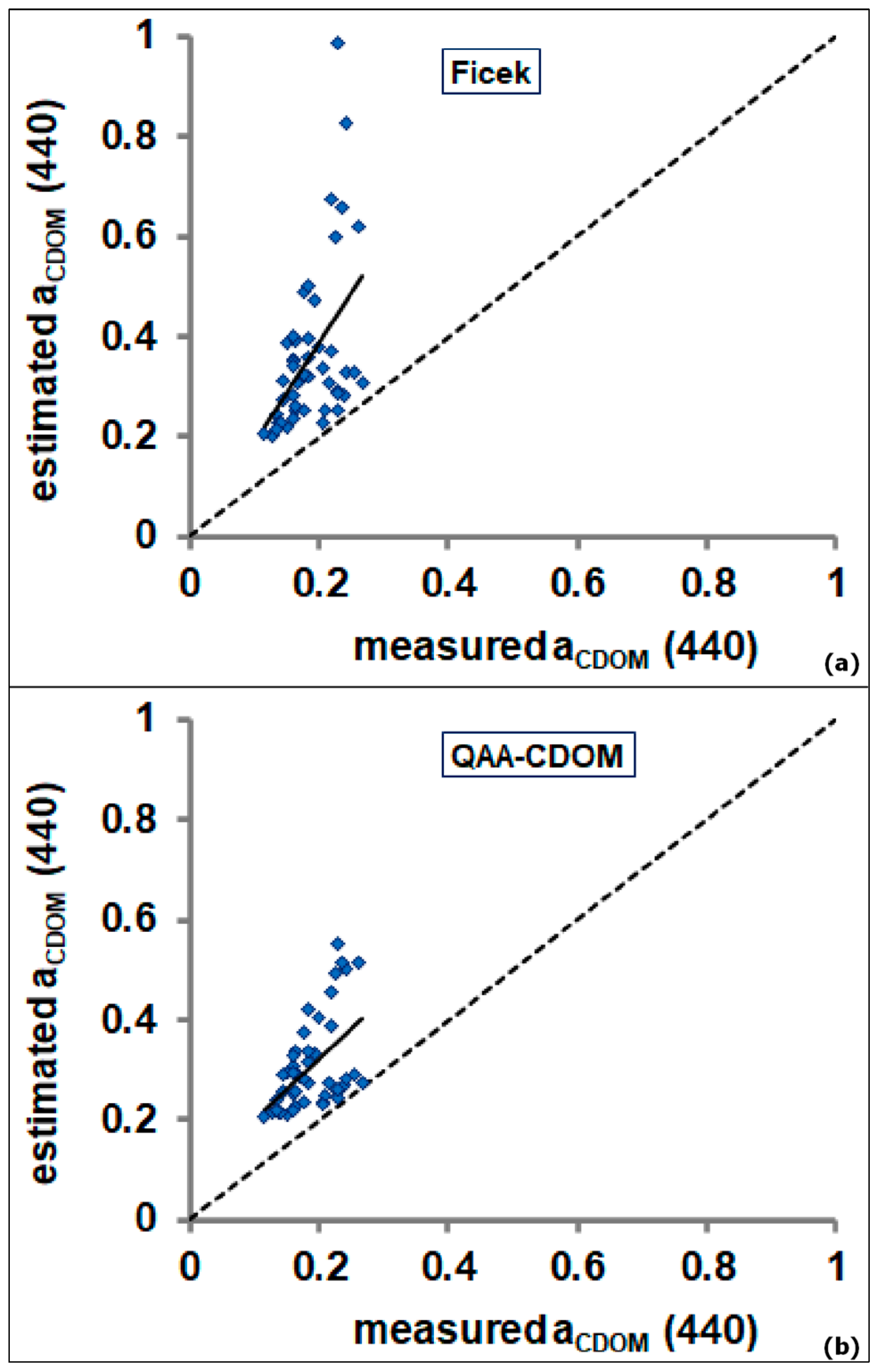
3.1. Assessment of a_CDOM (440) Algorithms

The two a_CDOM (440) algorithms [14,27] revealed poor suitability in retrieving accurate a_CDOM (440) estimations for the PL waters (a_CDOM (440) < 1 m⁻¹). The match-up analysis exhibited a clear overestimation for both the two models, as shown in Figure 3a,b.

The regression indices and error metrics for the two algorithms are reported in

Table 4. Regression indices and error metrics for the Ficek et al. [14] and QAA-CDOM [27] algorithms. * Represents a statistically significant p-value < 0.001.

Band Ratio	R2	r	APD	RMSE	n
Ficek et al. [14]	0.23 *	1.93	93.03	0.22	48
QAA-CDOM [27]	0.26 *	1.65	65.15	0.14	48

.

The two a_CDOM (440) models exhibited low performance, with R² between 0.23 and 0.26 and a strong overestimation and were proved by the r values ranging between 1.65 and 1.93 as well as the high values of APD (65.15–93.03%) and RMSE (0.14–0.22 m⁻¹).

The achieved results suggested the need to define a customized a_CDOM (440) model that accounts for the PL optical properties. Considering the lack of measured in situ IOPs (e.g., phytoplankton absorption coefficient, a_ph(λ) and/or particulate backscattering, and b_bp (λ)), we aimed at developing a customized a_CDOM (440) model based on an empirical-style algorithm by adopting the following cal/val procedures.

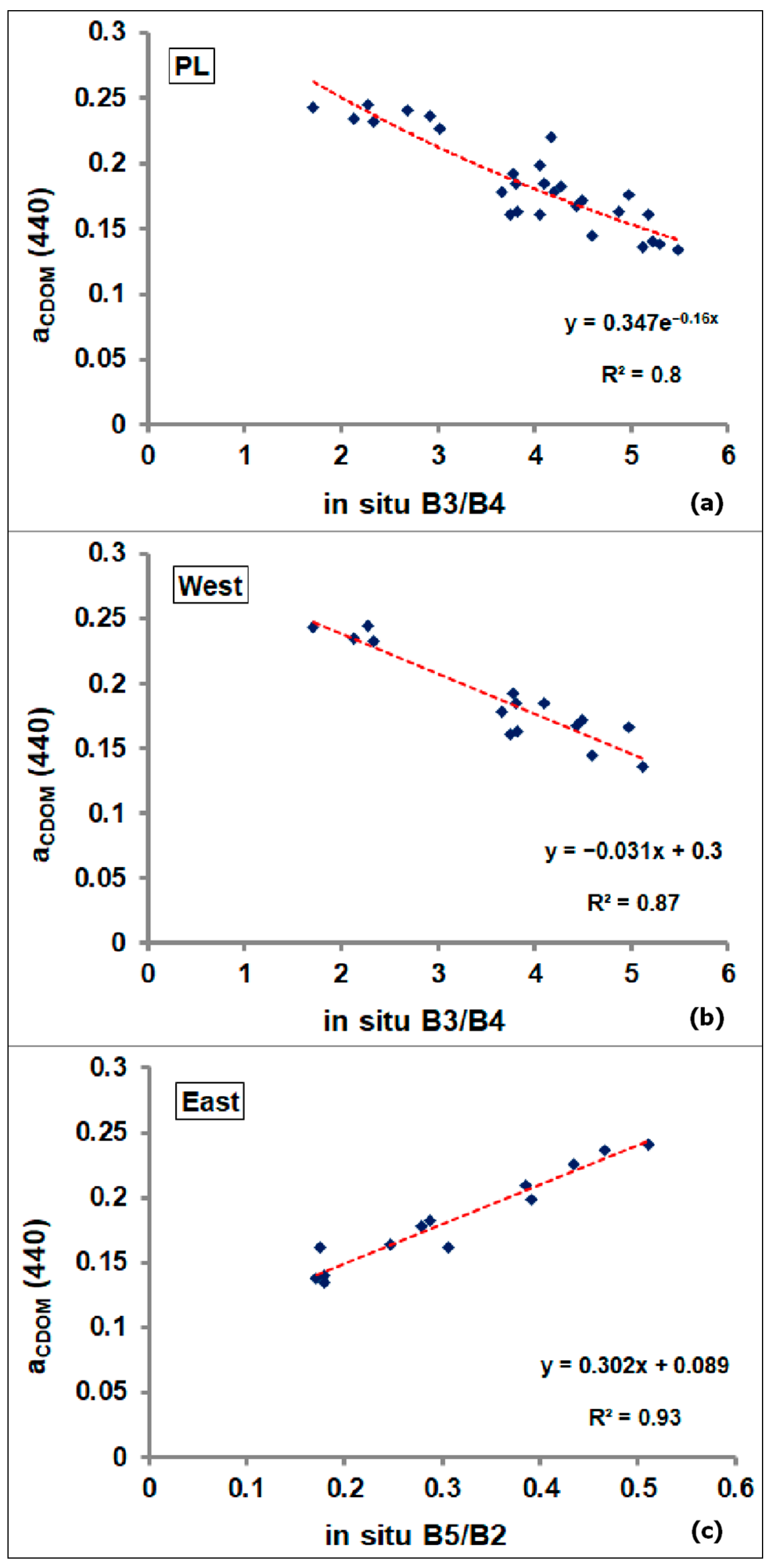
3.2. Model Calibration with In Situ Rrs(λ) Data

Within the calibration phase, the most suitable mathematical functions were assessed to establish relationships between in situ Rrs_e (i.e., equivalent Rrs for S2-MSI bands) band ratios and measured a_CDOM (440) values. Four literature band ratios (within the Blue–Red spectral range), namely B3/B4 [33], B3/B5 [36], B4/B2 [8], and B5/B2 [30], were retained for regression analyses. For each band ratio, the best-fit functions (i.e., linear, exponential, and power) recording the highest regression scores are reported in

Table 5. Calibration models for retrieving a_CDOM (440) based on in situ S2-MSI-simulated band ratios. * Represents a statistically significant p-value < 0.001.

Dataset	Band Ratio	Function	Calibration Model	R2	RMSE	n
PL	B3/B4	exponential	y = 0.347 × exp(−0.16x)	0.8 *	0.016	28
	B3/B5	linear	y = −0.016x + 0.269	0.79 *	0.0161	28
	B4/B2	power	y = 0.291x0.537	0.79 *	0.0162	28
	B5/B2	power	y = 0.268x0.348	0.75 *	0.0181	28
West subset	B3/B4	linear	y = −0.031x + 0.3	0.87 *	0.012	15
	B3/B5	linear	y = −0.015x + 0.262	0.84 *	0.0147	15
	B4/B2	power	y = 0.275x0.505	0.79 *	0.0149	15
	B5/B2	power	y = 0.251x0.312	0.78 *	0.0158	15
East subset	B3/B4	exponential	y = 0.424 × exp(−0.2x)	0.88 *	0.0121	13
	B3/B5	linear	y = −0.019x + 0.293	0.88 *	0.0122	13
	B4/B2	exponential	y = 0.091 × exp(1.68x)	0.92 *	0.009	13
	B5/B2	linear	y = 0.302x + 0.089	0.93 *	0.009	13

with the distinction between the whole PL and the two subregions.

From Table 5, all the best fit functions generally showed a high determination coefficient (R² ≥ 0.75) between in situ S2-MSI-simulated band ratios and a_CDOM (440). However, when analysis was conducted according to the sub-region division (West and East subset), a further improvement in the correlation was achieved. Based on such a subset distinction, R² shifted from a maximum of 0.8 (for the whole PL) to a maximum of 0.93 and RMSE from a minimum of 0.016 to a minimum of 0.009 m⁻¹ recorded in the East subset. Focusing on the different band ratios, B3/B4 showed the best regression metrics in the PL and West subsets via the exponential and linear best-fit functions, respectively (Figure 4a,b). Otherwise, a linear relationship between B5/B2 and a_CDOM (440) recorded the best performance in the East subset, as shown in Figure 4c.

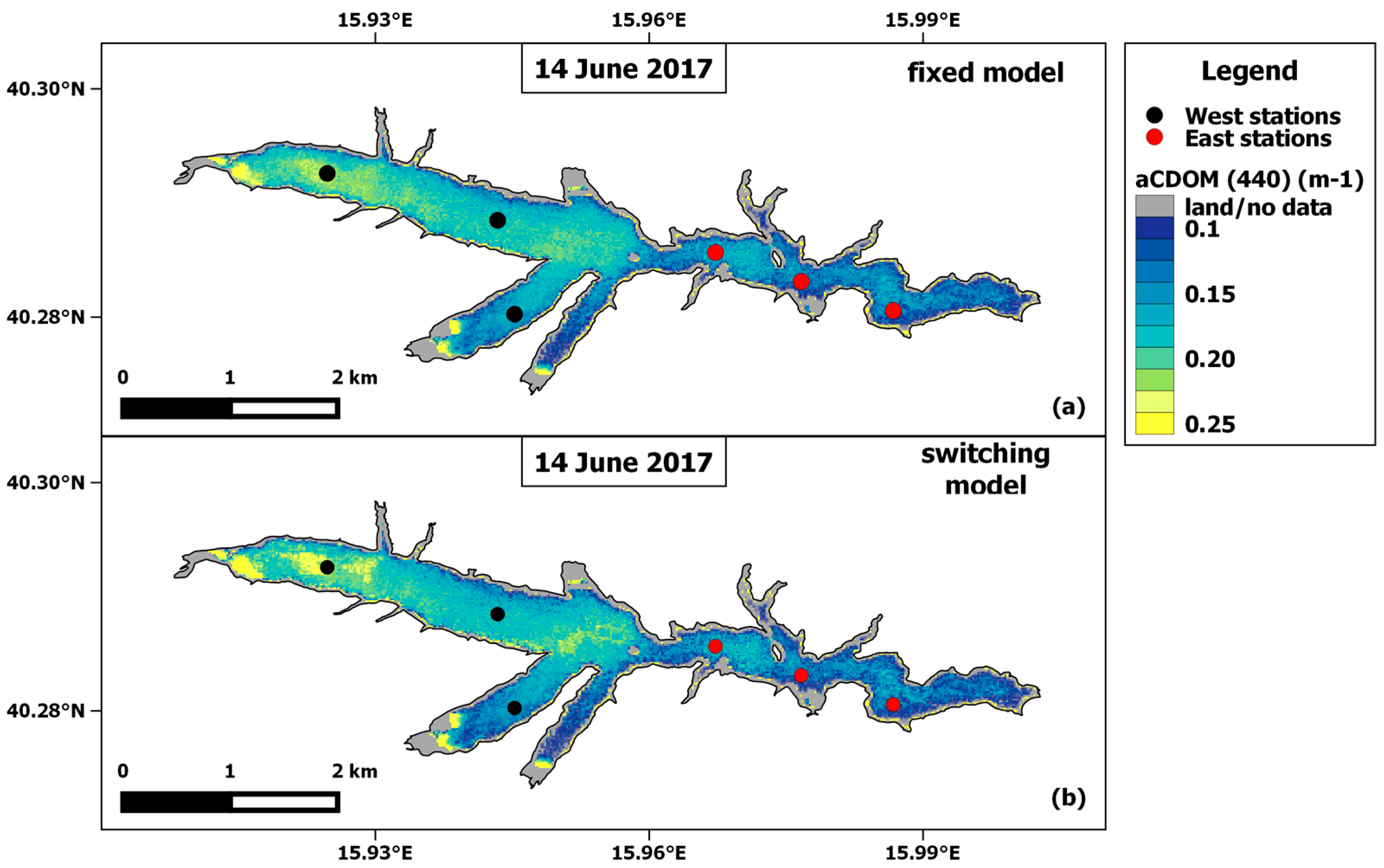
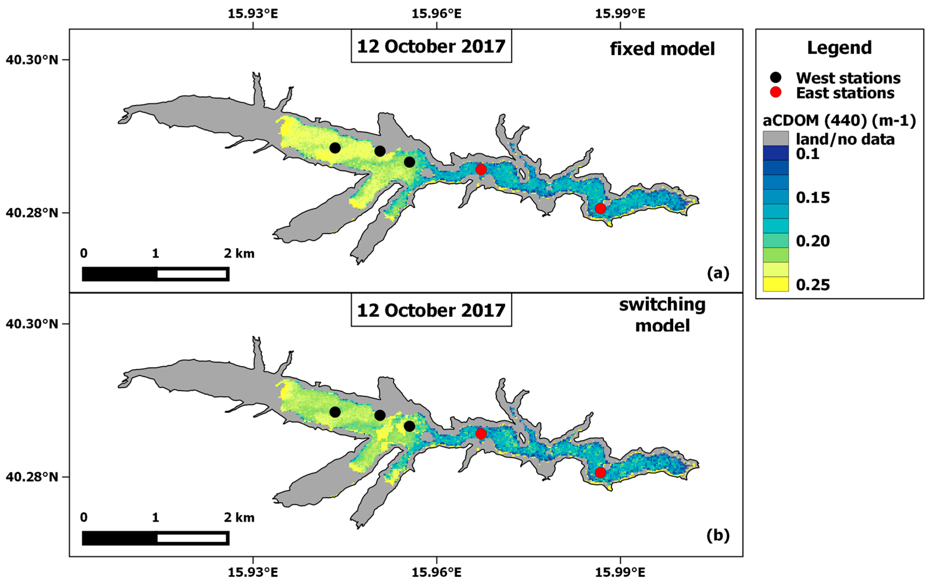
3.3. Model Validation with S2-MSI Data

As a first step of the validation phase, a specific match-up analysis was performed to evaluate the accuracy of the S2-MSI-derived band ratios with the corresponding in situ ones. According to the previously defined temporal criterion (i.e., ±3 h), only the S2-MSI-Rrs(λ) imagery acquired on 14 June 2017 and 12 October 2017 were retained for such an analysis. Figure 5 shows the match-up results for the following band ratios, namely B3/B4, B3/B5, B4/B2, and B5/B2.

The regression indices and error metrics for the investigated band ratios are listed in

Table 6. Regression coefficients and error metrics for the four band ratios considered. * Represents a statistically significant p-value < 0.001.

Band Ratio	R2	r	APD	%RMSE
B3/B4	0.77 *	1.03	9.86	11.91
B3/B5	0.74 *	0.89	16.90	23.88
B4/B2	0.94 *	1.15	15.94	19.98
B5/B2	0.78 *	1.41	41.62	48.25

.

All the four band ratios showed acceptable regression indices with a determination coefficient R² ≥ 0.74. Most of the scatterplots revealed a quite good correlation (with r values between 0.89 and 1.15), except for the B5/B2 ratio, which exhibits a clear overestimation (r = 1.41).

The error metrics highlighted clear differences among the investigated band ratios thus showing the best accuracy of the B3/B4 band ratio (APD of 9.86%) and the worst one for B5/B2 (%RMSE of 48.25%). Such results revealed that the B5/B2-based calibration model is not suitable for exportation on S2-MSI data as it could determine large APD or RMSE values in the S2-MSI-derived a_CDOM (440) retrievals. Although the in situ B5/B2 revealed the best regression metrics of calibration for the East subset, we adopted, for validation, the B3/B4-based a_CDOM (440) model (via exponential best fit), ensuring a comparable score in the regression rank (Table 5).

Based on the achieved results, we selected the most suitable a_CDOM (440) calibration models for the final validation phase. The three a_CDOM (440) models refer to the whole PL, the West and East subset, respectively, and are defined as following:

$${\mathrm{a}}_{\mathrm{C}\mathrm{D}\mathrm{O}\mathrm{M}}\left(440\right)=0.347\times \mathrm{e}\mathrm{x}\mathrm{p}\left[-0.16\times \left(\frac{\mathrm{B}3}{\mathrm{B}4}\right)\right],$$

(12)

$${\mathrm{a}}_{\mathrm{C}\mathrm{D}\mathrm{O}\mathrm{M}}\left(440\right)=-0.031\left(\frac{\mathrm{B}3}{\mathrm{B}4}\right)+0.3,$$

(13)

$${\mathrm{a}}_{\mathrm{C}\mathrm{D}\mathrm{O}\mathrm{M}}\left(440\right)=0.424\times \mathrm{e}\mathrm{x}\mathrm{p}\left[-0.2\times \left(\frac{\mathrm{B}3}{\mathrm{B}4}\right)\right],$$

(14)

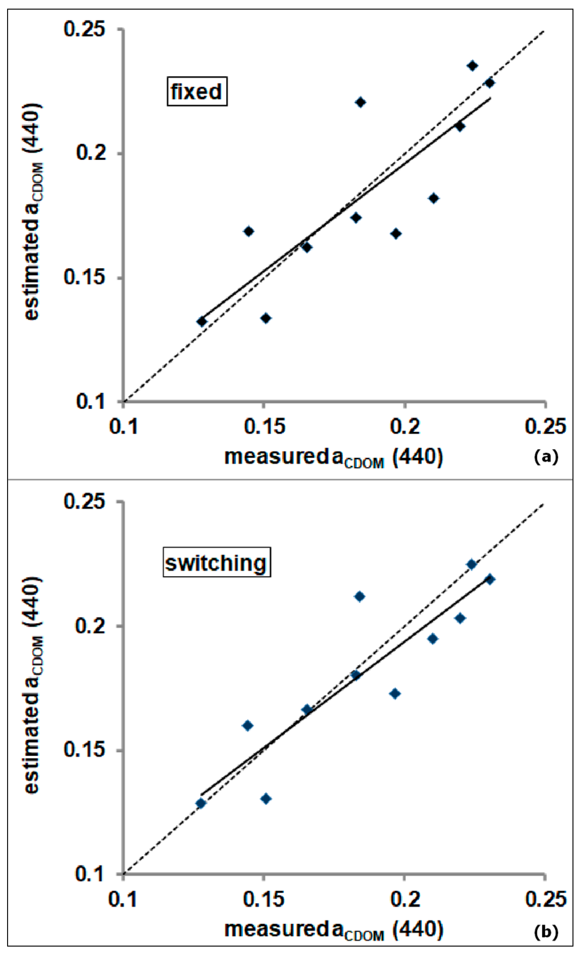
Fixed vs. Switchable PL-Tuned Models

The above-mentioned empirical relationships (Equations (12)–(14)) allowed at defining a fixed or switchable scheme of model for a_CDOM (440) retrievals by S2-MSI data. The a_CDOM (440) model defined by the Equation (12) represents a fixed scheme for all the pixels within the whole PL. The Equations (13) and (14) are used to define a “switchable” scheme of model on which the first algorithm (Equation (13)) is applied to the West subset pixels, while the second one (Equation (14)) to the East subset pixels. By exploiting an informative layer relied on a pixel membership to the two sub-regions (Figure 2), one of the two algorithms (i.e., Equation (13) or (14)) is alternatively implemented and automatically applied.

Figure 6 and Figure 7 show the S2-MSI a_CDOM (440) maps of 14 June 2017 and 12 October 2017 used for validation match-ups of the fixed (Equation (12) and switching (Equations (13) and (14)) a_CDOM (440) models, respectively.

Looking at Figure 6 and Figure 7, PL is generally characterized by low-CDOM waters (a_CDOM (440) ≤ 0.25 m⁻¹) with higher values in autumn than in summer as expected for reservoirs impacted by river flow fluctuations. Regardless of the model considered, a_CDOM (440) shows a well-defined spatial variability with higher values in the PL’s Western side than the Eastern as already noted by the in situ a_CDOM (440) measurements (Table 2).

Among the two investigated models, the switching model exhibited, on 14 June 2017, more pixels with higher a_CDOM (440) values (depicted in yellow in Figure 6b) in the West sub-region. On 12 October 2017, the fixed model showed higher a_CDOM (440) values (≈0.25 m⁻¹) spatially distributed over the PL west-central zone. On both the validation days the East subset exhibited comparable a_CDOM (440) spatial patterns with values not higher than 0.15–0.17 m⁻¹.

Both models showed a good agreement between estimated and measured a_CDOM (440), even if the switching model performed better than the fixed one, exhibiting a higher determination coefficient R² (0.80 against 0.7), as shown in Figure 8a,b.

The regression indices and error metrics for the two PL-tuned a_CDOM (440) models are summarized in

Table 7. Regression indices and error metrics of the two PL-tuned a_CDOM (440) models. * Represents a statistically significant p-value < 0.001.

Type	Dataset	CDOM Algorithm	R2	r	RMSE	%RMSE	APD
fixed	PL	exponential	0.7 *	0.98	0.0194	10.52	8.75
switching	West	linear	0.8 *	0.99	0.0155	8.38	6.79
	East	exponential

.

As shown in Table 7, both customized a_CDOM (440) models exhibited APD values well below 10%, confirming a satisfactory accuracy in a_CDOM (440) retrievals. Within an in-depth analysis, the implementation of a switching a_CDOM (440) model (Equations (9) and (10)) allowed for a further improvement of the accuracy scores with APD decreasing from 8.75% to 6.79% and RMSE from 0.0194 m⁻¹ to 0.0155 m⁻¹.

Based on these findings, the adoption of a TSM-driven sub-region division of PL resulted in a suitable methodological approach to reach more accurate a_CDOM (440) retrievals.

4. Discussion

Retrieving CDOM estimations and understanding its variability is crucial for monitoring and managing inland waters. CDOM retrievals in such waters are affected by different variables, such as hydrology, topography, and interactions between bio-optical in-water constituents [60,61]. Within this framework, different studies [62,63,64,65,66] have suggested the adoption of optical water classifications to improve retrieval models and/or define class-specific algorithms for bio-optical parameters, such as CDOM. Most of these studies have mainly divided waters into two types, namely clear and turbid, based on different indices or turbidity (or TSM values) levels [8,67]. Such fixed threshold approaches are site-dependent and result poorly suitable to be exported in other geographical regions with different turbidity conditions. The TSM-driven unsupervised classification proposed by Ciancia et al. [40] allowed for the overcoming of these limitations, because of its self-adaptive rationale that is not based on site-specific in situ data [40]. Within the classification scheme, the exploitation of multi-year TSM climatological monthly means as input spectral bands allowed for inherently incorporating information on TSM-connected forcings. Seasonal fluctuations of river discharges and bathymetry-induced erosion/sediment resuspension phenomena influenced the derived TSM climatological patterns [40]. Although the PL sub-division was methodologically obtained through a TSM-driven classification, the identification of sub-regions (Figure 2) was induced also by the eastward changes of topographic (i.e., bathymetry) and hydrological features (i.e., inflowing rivers) [40]. In this framework, the identification of areas exposed to different hydrological, topographic, and optical properties can allow for adopting more rigorous cal/val procedures aimed at refining CDOM algorithms and achieving more accurate estimations.

4.1. CDOM Modelling

The development of a PL-customized a_CDOM (440) model requires a preliminary performance assessment of the already published algorithms/models, considering there is no algorithm suitable for lakes at the global scale [56].

Among the empirical and semi-analytical algorithms, we selected two a_CDOM (440) models with the best performance rank for the algorithm and water type according to the recently published European Space Agency (ESA) report [56]. However, both the algorithms showed large overestimations (APD higher than 65.15%) of a_CDOM (440) for PL, confirming their sensitivity to changes in boundary conditions and suggesting the need to define a customized model. The lack of measured in situ IOPs (e.g., aph(λ) and/or bbp(λ)) did not allow for tuning a QAA-based model but the development of an empirical-style a_CDOM (440) algorithm. The high uncertainties recorded by the Ficek et al. algorithm [14] prompted us to not work on the tuning of regression coefficients but to consider both other literature band ratios and suitable best-fit functions (i.e., linear, exponential, and power) within the calibration phase.

The considered four band ratios could have profitably been adopted to estimate a_CDOM (440), as all the best-fit functions generally showed a good determination coefficient (R² ≥ 0.7) within regression analyses. The choice to separately consider the Western and Eastern sub-regions resulted profitable improvement in the performance of the a_CDOM (440) models with noticeable differences in regression and error metrics (R² up to 0.93 and RMSE of approximately 0.009 m⁻¹). The achieved results corroborated the need to identify sub-areas with similar bio-optical and topographical features to develop more customized and accurate a_CDOM (440) models. However, only the match-up analysis between S2-MSI-derived and in situ band ratios allowed for a clear selection of the most suitable one for exportability on S2-MSI data. Such an analysis revealed the B3/B4 band ratio as the most suitable for estimating a_CDOM (440) by S2-MSI data with good accuracy (APD of 9.86%). On the other hand, the Blue-based band ratios (i.e., B5/B2) showed minor capabilities for this purpose, probably due to the proven lower accuracy of the atmospheric correction at the blue wavelengths [12,40]. Furthermore, in this spectral region, the overlapping of phytoplankton (i.e., chlorophyll-a) and suspended matter (i.e., TSM) absorption spectra with that of CDOM could make difficult its retrievals in inland water bodies [68,69]. Selecting a relatively longer wavelength (>600 nm) as the denominator in the band ratio proved to significantly improve the accuracy of the empirical models in inland waters [29]. Since TSM usually presents high backscattering at these longer wavelengths, the exploitation of Red/Near Infrared bands allows for better accounting for particulate matter [70].

As per the validation phase, the two proposed model configurations (i.e., fixed or switching) ensured both satisfactory results with APD values well below 10%. Within a comparative analysis between the customized a_CDOM (440) models, the switching scheme showed a better performance (with a minimum APD value of 6.79%) but required a further step in satellite data processing. Although the switching model needs a preliminary informative layer to work (i.e., map of the PL sub-regions), its dynamic and automated algorithm selection allows for exploiting the complementarity of two optimization algorithms by switching between them through the pixel-based membership to the two sub-regions. Despite its good accuracy, the customized switching model should be cautionary adopted especially close to the deltaic and shallower PL’s Western zone. In this sub-region, water level drawdown could determine areas of emergent bottom with frequent episodes of erosion and/or deposition [40]. Increases in reflectance contribution due to bottom and possible emergent vegetation could cause sources of noise in the Rrs(λ) spectra with potential implications on the derived switching a_CDOM (440) model.

4.2. Future Developments

This work aimed at defining a PL-customized switching model for a_CDOM (440) retrievals by S2-MSI data. From a future perspective, the adoption of a B3/B4-based a_CDOM (440) model could enable its easy exportability on Landsat 8/9 (L8/9)-Operational Land Imager (OLI). In particular, the spectral proximity of the S2-MSI Green (560 nm) and Red (665 nm) bands to the corresponding L8/9-OLI ones (at 561 nm and 655 nm, respectively) should facilitate the inter-calibration procedure to develop an MSI–OLI combined dataset of a_CDOM (440) retrievals [40]. The joint exploitation of L8/9-OLI and S2-MSI data can contribute to minimizing any acquisition gap, thus ensuring an average revisit time of 2.9 days [71]. Finally, the potential exportability of such a switching a_CDOM (440) model on Landsat8/9-OLI data can provide great advantages also for water quality monitoring [72] aimed at ensuring the good quality status of water bodies, as requested by the Water Framework Directive (WFD, 2000/60/EC and amendments).

Furthermore, the OLI-like spectral configuration (especially for the Red and Green bands) of long-term satellite-sensor systems such as Landsat 5 Thematic Mapper (1984–2011) and Landsat 7 Enhance Thematic Mapper plus (1999–2022) can allow for a potential investigation of about 40-year a_CDOM (440) data [40]) enabling the assessment of climate-related or human-induced PL water quality changes.

In this framework, an open challenge remains the assessment of the potential effects of land transformation on inland water quality based on long-term analysis [73]. Areas surrounding artificial lakes have been subjected to different land use/cover dynamics in the last 30 years. A progressive forest expansion has been observed, mainly determined by land abandonment phenomena of less-favored agricultural areas [74]. Variations in soil structure and land use patterns can affect ecological, geochemical processes and hydrological variables (e.g., surface runoff, watershed precipitation, and river discharges) whose fluctuations usually affect CDOM variability [75,76]. Within a long-term analysis, understanding the potential relationship between land use changes and CDOM inter-annual variability plays a key role in considering the increasing inflow of terrestrial and anthropogenic CDOM into downstream-linked reservoirs [77].

5. Conclusions

In this study, we defined a PL-tuned a_CDOM (440) model by S2-MSI data adopting a previously achieved classification scheme on satellite TSM data [40].

The unsatisfactory performance (R² ≤ 0.26 and APD ≥ 65.15%) of two published a_CDOM (440) algorithms (i.e., Ficek et al. [14] and QAA_CDOM [27]) suggested the development of a PL-customized version of S2-MSI a_CDOM (440) model by using in situ radiometric data and a_CDOM (440) measurements.

The regression analyses between in situ band ratios and a_CDOM (440) measurements allowed for defining the most suitable a_CDOM (440) calibration models. The Green-to-Red (B3/B4 and B3/B5) and Red-to-Blue (B4/B2 and B5/B2) band ratios showed generally good performance (R² ≥ 0.75), further improved when analysis was conducted according to the sub-region division (R² up to 0.93 and a minimum RMSE of approximately 0.009 m⁻¹). Match-ups between S2-MSI-derived and in situ band ratios revealed the potential exportability of such calibration models on S2-MSI data. The unsatisfactory accuracy by B5/B2 and the good performance of B3/B4 resulted in the validation of two B3/B4-based a_CDOM (440) models, namely the fixed and the switching one, which is based on a pixel membership to the two PL sub-regions identified by the TSM-driven classification. Both customized a_CDOM (440) models exhibited satisfactory accuracy in a_CDOM (440) retrievals, with APD values well below 10%. Within an in-depth analysis, the switching model recorded an improved accuracy with APD decreasing from 8.75% to 6.79% and RMSE from 0.0194 m⁻¹ to 0.0155 m⁻¹ as well.

Based on the achieved findings, the identification of areas exposed to different TSM patterns, and hydrological and topographical features can allow for adopting more rigorous cal/val procedures aimed at refining algorithms and achieving more accurate a_CDOM (440) retrievals.

References

1. Carlson, C.A.; Ducklow, H.W.; Michaels, A.F. Annual flux of dissolved organic carbon from the euphotic zone in the northwestern Sargasso Sea. Nature 1994, 371, 405–408. [Google Scholar] [CrossRef]
2. Karlsson, J.; Byström, P.; Ask, J.; Ask, P.; Persson, L.; Jansson, M. Light limitation of nutrient-poor lake ecosystems. Nature 2009, 460, 506–509. [Google Scholar] [CrossRef]
3. Deininger, A.; Faithfull, C.L.; Bergström, A.K. Phytoplankton response to whole lake inorganic N fertilization along a gradient in dissolved organic carbon. Ecology 2017, 98, 982–994. [Google Scholar] [CrossRef]
4. Fee, E.J.; Hecky, R.E.; Kasian, S.E.M.; Cruikshank, D.R. Effects of lake size, water clarity, and climatic variability on mixing depths in Canadian Shield lakes. Limnol. Oceanogr. 1996, 41, 912–920. [Google Scholar] [CrossRef]
5. Houser, J.N. Water color affects the stratification, surface temperature, heat content, and mean epilimnetic irradiance of small lakes. Can. J. Fish. Aquat. Sci. 2006, 63, 2447–2455. [Google Scholar] [CrossRef]
6. Brezonik, P.; Arnold, W. Water Chemistry: An Introduction to the Chemistry of Natural and Engineered Aquatic Systems; Oxford University Press: New York, NY, USA, 2011. [Google Scholar]
7. Herzsprung, P.; von Tümpling, W.; Hertkorn, N.; Harir, M.; Büttner, O.; Bravidor, J.; Friese, K.; Schmitt-Kopplin, P. Variations of DOM quality in inflows of a drinking water reservoir: Linking of van Krevelen diagrams with EEMF spectra by rank correlation. Environ. Sci. Technol. 2012, 46, 5511–5518. [Google Scholar] [CrossRef]
8. Xu, J.; Fang, C.; Gao, D.; Zhang, H.; Gao, C.; Xu, Z.; Wang, Y. Optical models for remote sensing of chromophoric dissolved organic matter (CDOM) absorption in Poyang Lake. ISPRS J. Photogramm. Remote Sens. 2018, 142, 124–136. [Google Scholar] [CrossRef]
9. Fichot, C.G.; Downing, B.D.; Bergamaschi, B.A.; Windham-Myers, L.; Marvin-DiPasquale, M.; Thompson, D.R.; Gierach, M.M. High-resolution remote sensing of water quality in the San Francisco Bay–Delta Estuary. Environ. Sci. Technol. 2016, 50, 573–583. [Google Scholar] [CrossRef]
10. Griffin, C.G.; McClelland, J.W.; Frey, K.E.; Fiske, G.; Holmes, R.M. Quantifying CDOM and DOC in major Arctic rivers during ice-free conditions using Landsat TM and ETM+ data. Remote Sens. Environ. 2018, 209, 395–409. [Google Scholar] [CrossRef]
11. D’Sa, E.J.; Miller, R.L. Bio-optical properties in waters influenced by the Mississippi River during low flow conditions. Remote Sens. Environ. 2003, 84, 538–549. [Google Scholar] [CrossRef]
12. Kutser, T.; Pierson, D.C.; Kallio, K.Y.; Reinart, A.; Sobek, S. Mapping lake CDOM by satellite remote sensing. Remote Sens. Environ. 2005, 94, 535–540. [Google Scholar] [CrossRef]
13. Mannino, A.; Russ, M.E.; Hooker, S.B. Algorithm development and validation for satellite-derived distributions of DOC and CDOM in the US Middle Atlantic Bight. J. Geophys. Res. Ocean. 2008, 113, C07051. [Google Scholar] [CrossRef]
14. Ficek, D.; Zapadka, T.; Dera, J. Remote sensing reflectance of Pomeranian lakes and the Baltic. Oceanologia 2011, 53, 959–970. [Google Scholar] [CrossRef]
15. Lee, Z.; Carder, K.L.; Arnone, R.A. Deriving inherent optical properties from water color: A multiband quasi-analytical algorithm for optically deep waters. Appl. Opt. 2002, 41, 5755–5772. [Google Scholar] [CrossRef]
16. Lee, Z.; Weidemann, A.; Kindle, J.; Arnone, R.; Carder, K.L.; Davis, C. Euphotic zone depth: Its derivation and implication to ocean-color remote sensing. J. Geophys. Res. Ocean. 2007, 112, C03009. [Google Scholar] [CrossRef]
17. Maritorena, S.; Siegel, D.A.; Peterson, A.R. Optimization of a semianalytical ocean color model for global-scale applications. Appl. Opt. 2002, 41, 2705–2714. [Google Scholar] [CrossRef]
18. Werdell, P.J.; Franz, B.A.; Bailey, S.W.; Feldman, G.C.; Boss, E.; Brando, V.E.; Dowell, M.; Hirata, T.; Lavender, S.J.; Lee, Z.; et al. Generalized ocean color inversion model for retrieving marine inherent optical properties. Appl. Opt. 2013, 52, 2019–2037. [Google Scholar] [CrossRef]
19. Ruescas, A.B.; Hieronymi, M.; Mateo-Garcia, G.; Koponen, S.; Kallio, K.; Camps-Valls, G. Machine learning regression approaches for colored dissolved organic matter (CDOM) retrieval with S2-MSI and S3-OLCI simulated data. Remote Sens. 2018, 10, 786. [Google Scholar] [CrossRef]
20. Zhao, J.; Cao, W.; Xu, Z.; Ai, B.; Yang, Y.; Jin, G.; Wang, G.; Zhou, W.; Chen, Y.; Chen, H.; et al. Estimating CDOM concentration in highly turbid estuarine coastal waters. J. Geophys. Res. Ocean. 2018, 123, 5856–5873. [Google Scholar] [CrossRef]
21. Pahlevan, N.; Smith, B.; Alikas, K.; Anstee, J.; Barbosa, C.; Binding, C.; Bresciani, M.; Cremella, B.; Giardino, C.; Gurlin, D.; et al. Simultaneous retrieval of selected optical water quality indicators from Landsat-8, Sentinel-2, and Sentinel-3. Remote Sens. Environ. 2022, 270, 112860. [Google Scholar] [CrossRef]
22. Sagan, V.; Peterson, K.T.; Maimaitijiang, M.; Sidike, P.; Sloan, J.; Greeling, B.A.; Maaluf, S.; Adams, C. Monitoring inland water quality using remote sensing: Potential and limitations of spectral indices, bio-optical simulations, machine learning, and cloud computing. Earth-Sci. Rev. 2020, 205, 103187. [Google Scholar] [CrossRef]
23. Pitarch, J.; Vanhellemont, Q. The QAA-RGB: A universal three-band absorption and backscattering retrieval algorithm for high resolution satellite sensors. Development and implementation in ACOLITE. Remote Sens. Environ. 2021, 265, 112667. [Google Scholar] [CrossRef]
24. Wang, Y.; Shen, F.; Sokoletsky, L.; Sun, X. Validation and calibration of QAA algorithm for CDOM absorption retrieval in the Changjiang (Yangtze) estuarine and coastal waters. Remote Sens. 2017, 9, 1192. [Google Scholar] [CrossRef]
25. Colella, S.; Brando, V.E.; Cicco, A.D.; D’Alimonte, D.; Forneris, V.; Bracaglia, M. Ocean Colour Production Centre, Ocean Colour Mediterranean and Black Sea Observation Product. Copernicus Marine Environment Monitoring Centre. Quality Information Document. 2021. Available online: https://catalogue.marine.copernicus.eu/documents/QUID/CMEMS-OMI-QUID-HEALTH-CHL-BLKSEA-OCEANCOLOUR.pdf (accessed on 23 June 2023).
26. Jackson, T. ESA Ocean Colour Climate Change Initiative—Phase 3. Product User Guide for v5.0 Dataset. 2020. Available online: https://docs.pml.space/share/s/okB2fOuPT7Cj2r4C5sppDg (accessed on 25 July 2023).
27. Zhu, W.; Yu, Q. Inversion of chromophoric dissolved organic matter from EO-1 Hyperion imagery for turbid estuarine and coastal waters. IEEE Trans. Geosci. Remote Sens. 2012, 51, 3286–3298. [Google Scholar] [CrossRef]
28. Dong, Q.; Shang, S.; Lee, Z. An algorithm to retrieve absorption coefficient of chromophoric dissolved organic matter from ocean color. Remote Sens. Environ. 2013, 128, 259–267. [Google Scholar] [CrossRef]
29. Zhu, W.; Yu, Q.; Tian, Y.Q.; Becker, B.L.; Zheng, T.; Carrick, H.J. An assessment of remote sensing algorithms for colored dissolved organic matter in complex freshwater environments. Remote Sens. Environ. 2014, 140, 766–778. [Google Scholar] [CrossRef]
30. Shang, Y.; Liu, G.; Wen, Z.; Jacinthe, P.A.; Song, K.; Zhang, B.; Lyu, L.; Li, S.; Wang, X.; Yu, X. Remote estimates of CDOM using Sentinel-2 remote sensing data in reservoirs with different trophic states across China. J. Environ. Manag. 2021, 286, 112275. [Google Scholar] [CrossRef]
31. Del Castillo, C.E.; Miller, R.L. On the use of ocean color remote sensing to measure the transport of dissolved organic carbon by the Mississippi River Plume. Remote Sens. Environ. 2008, 112, 836–844. [Google Scholar] [CrossRef]
32. Griffin, C.G.; Frey, K.E.; Rogan, J.; Holmes, R.M. Spatial and interannual variability of dissolved organic matter in the Kolyma River, East Siberia, observed using satellite imagery. J. Geophys.Res. Biogeosciences 2011, 116, G03018. [Google Scholar] [CrossRef]
33. Al-Kharusi, E.S.; Tenenbaum, D.E.; Abdi, A.M.; Kutser, T.; Karlsson, J.; Bergström, A.K.; Berggren, M. Large-scale retrieval of coloured dissolved organic matter in northern lakes using Sentinel-2 data. Remote Sens. 2020, 12, 157. [Google Scholar] [CrossRef]
34. Palmer, S.C.; Kutser, T.; Hunter, P.D. Remote sensing of inland waters: Challenges, progress and future directions. Remote Sens. Environ. 2015, 157, 1–8. [Google Scholar] [CrossRef]
35. Drusch, M.; Del Bello, U.; Carlier, S.; Colin, O.; Fernandez, V.; Gascon, F.; Hoersch, B.; Isola, C.; Laberinti, P.; Martimort, P.; et al. Sentinel-2: ESA’s optical high-resolution mission for GMES operational services. Remote Sens. Environ. 2012, 120, 25–36. [Google Scholar] [CrossRef]
36. Chen, J.; Zhu, W.; Tian, Y.Q.; Yu, Q.; Zheng, Y.; Huang, L. Remote estimation of colored dissolved organic matter and chlorophyll-a in Lake Huron using Sentinel-2 measurements. J. Appl. Remote Sens. 2017, 11, 036007. [Google Scholar] [CrossRef]
37. Toming, K.; Kutser, T.; Laas, A.; Sepp, M.; Paavel, B.; Nõges, T. First experiences in mapping lake water quality parameters with Sentinel-2 MSI imagery. Remote Sens. 2016, 8, 640. [Google Scholar] [CrossRef]
38. Faruolo, M.; Coviello, I.; Filizzola, C.; Lacava, T.; Pergola, N.; Tramutoli, V. A satellite-based analysis of the Val d’Agri Oil Center (southern Italy) gas flaring emissions. Nat. Hazards Earth Syst. Sci. 2014, 14, 2783–2793. [Google Scholar] [CrossRef]
39. Laneve, G.; Bruno, M.; Mukherjee, A.; Messineo, V.; Giuseppetti, R.; De Pace, R.; Magurano, F.; D’Ugo, E. Remote sensing detection of algal blooms in a lake impacted by petroleum hydrocarbons. Remote Sens. 2021, 14, 121. [Google Scholar] [CrossRef]
40. Ciancia, E.; Campanelli, A.; Lacava, T.; Palombo, A.; Pascucci, S.; Pergola, N.; Pignatti, S.; Satriano, V.; Tramutoli, V. Modeling and multi-temporal characterization of total suspended matter by the combined use of Sentinel 2-MSI and Landsat 8-OLI data: The Pertusillo Lake case study (Italy). Remote Sens. 2020, 12, 2147. [Google Scholar] [CrossRef]
41. Autorità Di Bacino Della Basilicata. Available online: http://www.adb.basilicata.it/adb/risorseidriche/diag_inv.asp?invaso=pertusillo (accessed on 23 March 2023).
42. Colella, A.; Fortunato, E. The Sedimentary Infill of the Pertusillo Freshwater Reservoir (Val d’Agri, Southern Italy). FEB Fresenius Environ. Bull. 2019, 23, 824–830. [Google Scholar]
43. Tou, J.T.; Gonzalez, R.C. Pattern Recognition Principles; Addison-Wesley: Boston, MA, USA, 1974. [Google Scholar]
44. Salvia, M.; Cornacchia, C.; Di Renzo, G.C.; Braccio, G.; Annunziato, M.; Colangelo, A.; Orifici, L.; Lapenna, V. Promoting smartness among local areas in a Southern Italian region: The Smart Basilicata Project. Indoor Built Environ. 2016, 25, 1024–1038. [Google Scholar] [CrossRef]
45. Strickland, J.D.; Parsons, T.R. A Practical Handbook of Seawater Analysis; Fisheries Research Board of Canada: Ottawa, ON, Canada, 1972. [Google Scholar]
46. UNESCO. Protocols for the Joint Global Ocean Flux Study (JGOFS) Core Measurements; UNESCO-IOC: Paris, France, 1994. [Google Scholar]
47. Mitchell, B.G.; Kahru, M.; Wieland, J.; Stramska, M. Determination of spectral absorption coefficient of particles, dissolved material and phytoplankton for discrete water samples. In Ocean Optics Protocols for Satellite Ocean Colour Sensor Validation; Fargion, G.S., Mueller, J.L., McClain, C.R., Eds.; NASA/TM-2003-211621/Rev4-Volume IV; NASA Goddard Space Flight Center: Greenbelt, MD, USA, 2003; pp. 39–64. [Google Scholar]
48. Bricaud, A.; Morel, A.; Prieur, L. Absorption by dissolvedorganicmatter of the sea (yellowsubstance) in the UV and visible domains. Limnol. Oceanogr. 1981, 26, 43–53. [Google Scholar] [CrossRef]
49. Grunert, B.K.; Mouw, C.B.; Ciochetto, A.B. Characterizing CDOM spectralvariabilityacross diverse regions and spectral ranges. Glob. Biogeochem. Cycles 2018, 32, 57–77. [Google Scholar] [CrossRef]
50. Mueller, J.L.; Fargion, G.S.; McClain, C.R. Ocean Optics Protocols for Satellite Ocean Color Sensor Validation, Revision 5: Biogeochemical and Bio-Optical Measurements and Data Analysis Protocols: Vol. 5; NASA Goddard Space Flight Space Center: Greenbelt, MD, USA, 2004; Volume 211621. [Google Scholar]
51. Lee, Z.P. Remote Sensing of Inherent Optical Properties: Fundamentals, Tests of Algorithms, and Applications; International Ocean Colour Coordinating Group (IOCCG): Hanover, NH, Canada, 2006. [Google Scholar]
52. ViewSpec Pro Software Manual, ASD Inc. 2008. Available online: http://www.grss-ieee.org/lep4/project_materials_for_web/viewspecpro_manual.pdf (accessed on 19 May 2022).
53. ESA’s Science Hub Web Portal. Available online: https://scihub.copernicus.eu (accessed on 18 May 2022).
54. ACOLITE Software. Available online: https://odnature.naturalsciences.be/remsem/acolite-forum (accessed on 9 May 2022).
55. Vanhellemont, Q.; Ruddick, K. Atmospheric Correction of Metre-Scale Optical Satellite Data for Inland and Coastal Water Applications. Remote Sens. Environ. 2018, 216, 586–597. [Google Scholar] [CrossRef]
56. Jiang, D.; Spyrakos, E. Technical Note: CDOM Algorithm Development for Global inland Waters. CCI-LAKES2-0006-TN-Issue 1.2. 2022. Available online: https://climate.esa.int/media/documents/CDOM_Techinical_Note_CCN-D-1_V1.2_final.pdf (accessed on 14 September 2023).
57. Sentinel-2 Spectral Response Functions (S2-SRF). Available online: https://sentinels.copernicus.eu/web/sentinel/user-guides/sentinel-2-msi/document-%20library/-/asset_publisher/Wk0TKajiISaR/content/sentinel-2a-spectral-responses (accessed on 7 April 2022).
58. Trigg, S.; Flasse, S. Characterizing the spectral-temporal response of burned savannah using in situ spectroradiometry and infrared thermometry. Int. J. Rem. Sens. 2000, 21, 3161–3168. [Google Scholar] [CrossRef]
59. Zibordi, G.; Voss, K. Protocols for Satellite Ocean Color Data Validation: In Situ Optical Radiometry; IOCCG Protocols Document; IOCCG: Hanover, NH, Canada, 2019. [Google Scholar]
60. Aulló-Maestro, M.E.; Hunter, P.; Spyrakos, E.; Mercatoris, P.; Kovács, A.; Horváth, H.; Preston, T.; Presing, M.; Palenzuela, J.T.; Tyler, A. Spatio-seasonal variability of chromophoric dissolved organic matter absorption and responses to photobleaching in a large shallow temperate lake. Biogeosciences 2017, 14, 1215–1233. [Google Scholar] [CrossRef]
61. Evans, C.D.; Futter, M.N.; Moldan, F.; Valinia, S.; Frogbrook, Z.; Kothawala, D.N. Variability in organic carbon reactivity across lake residence time and trophic gradients. Nat. Geosci. 2017, 10, 832–835. [Google Scholar] [CrossRef]
62. Shen, F.; Verhoef, W.; Zhou, Y.; Salama, M.S.; Liu, X. Satellite estimates of wide-range suspended sediment concentrations in Changjiang (Yangtze) estuary using MERIS data. Estuaries Coasts 2010, 33, 1420–1429. [Google Scholar] [CrossRef]
63. Moore, T.S.; Dowell, M.D.; Bradt, S.; Verdu, A.R. An optical water type framework for selecting and blending retrievals from bio-optical algorithms in lakes and coastal waters. Remote Sens. Environ. 2014, 143, 97–111. [Google Scholar] [CrossRef] [PubMed]
64. Jackson, T.; Sathyendranath, S.; Mélin, F. An improved optical classification scheme for the Ocean Colour Essential Climate Variable and its applications. Remote Sens. Environ. 2017, 203, 152–161. [Google Scholar] [CrossRef]
65. Jiang, D.; Matsushita, B.; Setiawan, F.; Vundo, A. An improved algorithm for estimating the Secchi disk depth from remote sensing data based on the new underwater visibility theory. ISPRS J. Photogramm. Remote Sens. 2019, 152, 13–23. [Google Scholar] [CrossRef]
66. Wang, S.; Li, J.; Zhang, B.; Lee, Z.; Spyrakos, E.; Feng, L.; Liu, C.; Zhao, H.; Wu, Y.; Zhu, L.; et al. Changes of water clarity in large lakes and reservoirs across China observed from long-term MODIS. Remote Sens. Environ. 2020, 247, 111949. [Google Scholar] [CrossRef]
67. Qing, S.; Cui, T.; Lai, Q.; Bao, Y.; Diao, R.; Yue, Y.; Hao, Y. Improving remote sensing retrieval of water clarity in complex coastal and inland waters with modified absorption estimation and optical water classification using Sentinel-2 MSI. Int. J. Appl. Earth Obs. Geoinf. 2021, 102, 102377. [Google Scholar] [CrossRef]
68. Gitelson, A.A.; Schalles, J.F.; Hladik, C.M. Remote chlorophyll-a retrieval in turbid, productive estuaries: Chesapeake Bay case study. Remote Sens. Environ. 2007, 109, 464–472. [Google Scholar] [CrossRef]
69. Odermatt, D.; Gitelson, A.; Brando, V.E.; Schaepman, M. Review of constituent retrieval in optically deep and complex waters from satellite imagery. Remote Sens. Environ. 2012, 118, 116–126. [Google Scholar] [CrossRef]
70. Yu, Q.; Tian, Y.Q.; Chen, R.F.; Liu, A.; Gardner, G.B.; Zhu, W. Functional linear analysis of in situ hyperspectral data for assessing CDOM in rivers. Photogramm. Eng. Remote Sens. 2010, 76, 1147–1158. [Google Scholar] [CrossRef]
71. Li, J.; Roy, D.P. A global analysis of Sentinel-2A, Sentinel-2B and Landsat-8 data revisit intervals and implications for terrestrial monitoring. Remote Sens. 2017, 9, 902. [Google Scholar] [CrossRef]
72. Chen, J.; Zhu, W.; Tian, Y.Q.; Yu, Q. Monitoring dissolved organic carbon by combining Landsat-8 and Sentinel-2 satellites: Case study in Saginaw River estuary, Lake Huron. Sci. Total Environ. 2020, 718, 137374. [Google Scholar] [CrossRef]
73. Cheng, C.; Zhang, F.; Shi, J.; Kung, H.T. What is the relationship between land use and surface water quality? A review and prospects from remote sensing perspective. Environ. Sci. Pollut. Res. 2022, 29, 56887–56907. [Google Scholar] [CrossRef]
74. Simoniello, T.; Coluzzi, R.; Imbrenda, V.; Lanfredi, M. Land cover changes and forest landscape evolution (1985–2009) in a typical Mediterranean agroforestry system (high Agri Valley). Nat. Hazards Earth Syst. Sci. 2015, 15, 1201–1214. [Google Scholar] [CrossRef]
75. Vitousek, P.M.; Mooney, H.A.; Lubchenco, J.; Melillo, J.M. Human domination of Earth’s ecosystems. Science 1997, 277, 494–499. [Google Scholar] [CrossRef]
76. Nickayin, S.S.; Coluzzi, R.; Marucci, A.; Bianchini, L.; Salvati, L.; Cudlin, P.; Imbrenda, V. Desertification risk fuels spatial polarization in ‘affected’and ‘unaffected’ landscapes in Italy. Sci. Rep. 2022, 12, 747. [Google Scholar] [CrossRef]
77. Drake, T.W.; Raymond, P.A.; Spencer, R.G. Terrestrial carbon inputs to inland waters: A current synthesis of estimates and uncertainty. Limnol. Oceanogr. Lett. 2018, 3, 132–142. [Google Scholar] [CrossRef]
78. Pope, R.M.; Fry, E.S. Absorption spectrum (380–700 nm) of pure water. II. Integrating cavity measurements. Appl. Opt. 1997, 36, 8710–8723. [Google Scholar] [CrossRef] [PubMed]
79. Kou, L.; Labrie, D.; Chylek, P. Refractive indices of water and ice in the 0.65-to 2.5-μm spectral range. Appl. Opt. 1993, 32, 3531–3540. [Google Scholar] [CrossRef] [PubMed]
80. Zhang, X.; Hu, L.; He, M.X. Scattering by pure seawater: Effect of salinity. Opt. Express 2009, 17, 5698–5710. [Google Scholar] [CrossRef] [PubMed]
Figure 1. On the left is the PL location and on the right is the magnification of the study area (reported in the WGS 84 Coordinate Reference System (CRS)). The main rivers/tributaries (continuous black lines) and the bathymetry (in blue tones) are depicted. The villages (black triangles) and the onshore oil field (i.e., Centro Olio Val d’Agri) close to PL are also reported.
Remotesensing 15 05718 g001
Figure 2. Map of the PL sub-regions derived from the ISODATA unsupervised classification (adapted from Ciancia et al. [40]). Dots represent the locations of the sampling stations designed for the in situ measurement campaigns. The yellow dots (from S1 to S6) are those falling into the PL western side while the red ones (from S7 to S10) are within the PL eastern side.
Remotesensing 15 05718 g002
Figure 3. Scatter plot of estimated versus measured aCDOM (440) for (a) the empirical [14] and (b) the semi-analytical [27] algorithms. The regression and 1:1 lines are depicted by the continuous and dashed lines, respectively.
Remotesensing 15 05718 g003
Figure 4. Most performing calibration models (in terms of R2 and RMSE) for the whole PL (a), the West (b), and East (c) subsets, respectively. The equations in the plots represent the mathematical “best-fitting” functions (dashed red line).
Remotesensing 15 05718 g004
Figure 5. S2-MSI band ratios versus in situ ones for (a) B3/B4, (b) B3/B5, (c) B4/B2, and (d) B5/B2. Note that the analysis was performed without distinction between sub-regions (i.e., West and East). The regression and 1:1 lines are depicted by the continuous and dashed lines, respectively.
Remotesensing 15 05718 g005
Figure 6. S2-MSI aCDOM (440) maps of 14 June 2017 for the CDOM fixed model (a) and the switching one (b), respectively. The black and red dots are the validation sampling stations falling into the West and East subsets, respectively.
Remotesensing 15 05718 g006
Figure 7. S2-MSI aCDOM (440) maps of 12 October 2017 for the CDOM fixed model (a) and the switching one (b), respectively. The black and red dots are the validation sampling stations falling into the West and East subsets, respectively.
Remotesensing 15 05718 g007
Figure 8. Validation match-ups of S2-MSI aCDOM (440) models based on a fixed PL-tuned algorithm (a) and on a switching PL-tuned one (b). The regression and 1:1 lines are depicted by the continuous and dashed lines, respectively.
Remotesensing 15 05718 g008