Noisy Remote Sensing Scene Classification via Progressive Learning Based on Multiscale Information Exploration

Abstract

Remote sensing (RS) scene classification has always attracted much attention as an elemental and hot topic in the RS community. In recent years, many methods using convolutional neural networks (CNNs) and other advanced machine-learning techniques have been proposed. Their performance is excellent; however, they are disabled when there are noisy labels (i.e., RS scenes with incorrect labels), which is inevitable and common in practice. To address this problem, some specific RS classification models have been developed. Although feasible, their behavior is still limited by the complex contents of RS scenes, excessive noise filtering schemes, and intricate noise-tolerant learning strategies. To further enhance the RS classification results under the noisy scenario and overcome the above limitations, in this paper we propose a multiscale information exploration network (MIEN) and a progressive learning algorithm (PLA). MIEN involves two identical sub-networks whose goals are completing the classification and recognizing possible noisy RS scenes. In addition, we develop a transformer-assistive multiscale fusion module (TAMSFM) to enhance MIEN’s behavior in exploring the local, global, and multiscale contents within RS scenes. PLA encompasses a dual-view negative-learning (DNL) stage, an adaptively positive-learning (APL) stage, and an exhaustive soft-label-learning (ESL) stage. Their aim is to learn the relationships between RS scenes and irrelevant semantics, model the links between clean RS scenes and their labels, and generate reliable pseudo-labels. This way, MIEN can be thoroughly trained under the noisy scenario. We simulate noisy scenarios and conduct extensive experiments using three public RS scene data sets. The positive experimental results demonstrate that our MIEN and PLA can fully understand RS scenes and resist the negative influence of noisy samples.

1. Introduction

As important earth observation data, remote-sensing (RS) images incorporate sufficient and diverse land covers and play an essential role in many fields. Exploring the valuable information within them according to the demands of various applications is always an open and hot topic. Among diverse interpretation techniques, RS scene classification is an elemental one, which aims to define semantic labels in line with the contents of RS scenes [1,2]. The accurate scene classification results are beneficial to different RS tasks and applications, such as image retrieval [3], land cover classification [4,5,6], hazard and environmental monitoring [7,8], resource exploration [9,10], etc.

Over the past decades, extensive methods have been proposed for RS scene classification. In the early stage, the low- and mid-level visual feature descriptors and traditional machine-learning methods were popular [11,12]. However, since those hand-crafted features cannot fully describe the complex contents within RS scenes and traditional machine-learning classifiers cannot fit the feature distributions adequately, the performance of the above methods is less than satisfactory. With the appearance of convolutional neural networks (CNNs), many CNN-based methods have been proposed for RS scene classification [13,14,15]. On the one hand, the intricate land covers within RS scenes can be represented owing to CNN’s strong feature learning capacity. On the other hand, by integrating feature learning and classification into an end-to-end framework, the classifiers embedded at the top of CNNs can follow feature distributions smoothly. Therefore, these CNN-based methods’ performance is excellent. Recently, the transformer [16,17] has been introduced into the RS scene classification community. Benefiting from the ability to perform long-range relation exploration, transformer-based methods have also achieved impressive results.

Despite the significant successes, a prerequisite exists, i.e., the manual ground truth of abundant RS scenes is correct and credible. Nevertheless, this hypothesis is not always true in practice [18,19,20], especially for RS images. First, manually labeling the big RS data is challenging, time-consuming, and labor-intensive. In addition, the practitioners should have professional knowledge. Second, the specific characteristics of RS scenes (i.e., land covers are diverse in type and large in volume) increase the annotation difficulty. Consequently, mislabeling RS scenes is unavoidable, and the produced noisy labels influence the scene classification negatively. Developing RS scene classification models with the consideration of noisy labels has become an urgent task.

Recently, some noise-tolerant methods have been developed for RS scene classification [21,22,23]. Although their performance is favorable, there is still room for improvement. First, the existing methods pay more attention to developing noise filtering or tolerance algorithms but ignore mining the RS scenes’ complex contents. This would limit their performance in RS scene classification. Second, filtering methods aim to eliminate the possible noisy samples so that the models can learn the correct information. However, some clean samples are also removed at the same time. This leads to information loss and degrades the behavior of classification models. Third, the noise tolerance methods are habituated to enhance the robustness of the models to the noisy labels by introducing specific learning strategies. However, these sophisticated learning schemes always bring problems of slow training speed and poor convergence, which impact the models’ practicability. Last but not least, they generally involve hard-to-tune and data set-dependent hyper-parameters, limiting their reliability and scalability.

To solve the above problems, we proposed a new multiscale information exploration network (MIEN) and a progressive learning algorithm (PLA) for noisy RS scene classification. MIEN consists of two identical networks, i.e., a classification sub-network and a teacher sub-network. Considering the complex contents of RS scenes, two sub-networks first adopt ResNet18 [24] as the backbone to capture the local messages hidden in RS scenes. Then, a transformer-assistive multiscale fusion module (TAMSFM) is developed to discover the global and multiscale knowledge within RS scenes. Incorporating them jointly, the rich and complete information can be mined from RS scenes for classification. To ensure MIEN can resist the noisy labels’ influence, a specific parameter-transmitting strategy is introduced. By learning the temporal information produced by the classification sub-network, the teacher sub-network can recognize the noisy samples smoothly. PLA is a noise tolerance optimization algorithm that incorporates three stages, including a dual-view negative-learning (DNL) stage, an adaptively positive-learning (APL) stage, and an exhaustive soft-label-learning (ESL) stage. Their main targets are learning the relationships between RS scenes and irrelevant semantics, modeling the links between clean RS scenes and their labels, and generating reliable pseudo-labels. Three learning stages are conducted in serial. After training MIEN by PLA, the RS scenes can be classified accurately under the noisy scenario. Our main contributions can be summarized as follows:

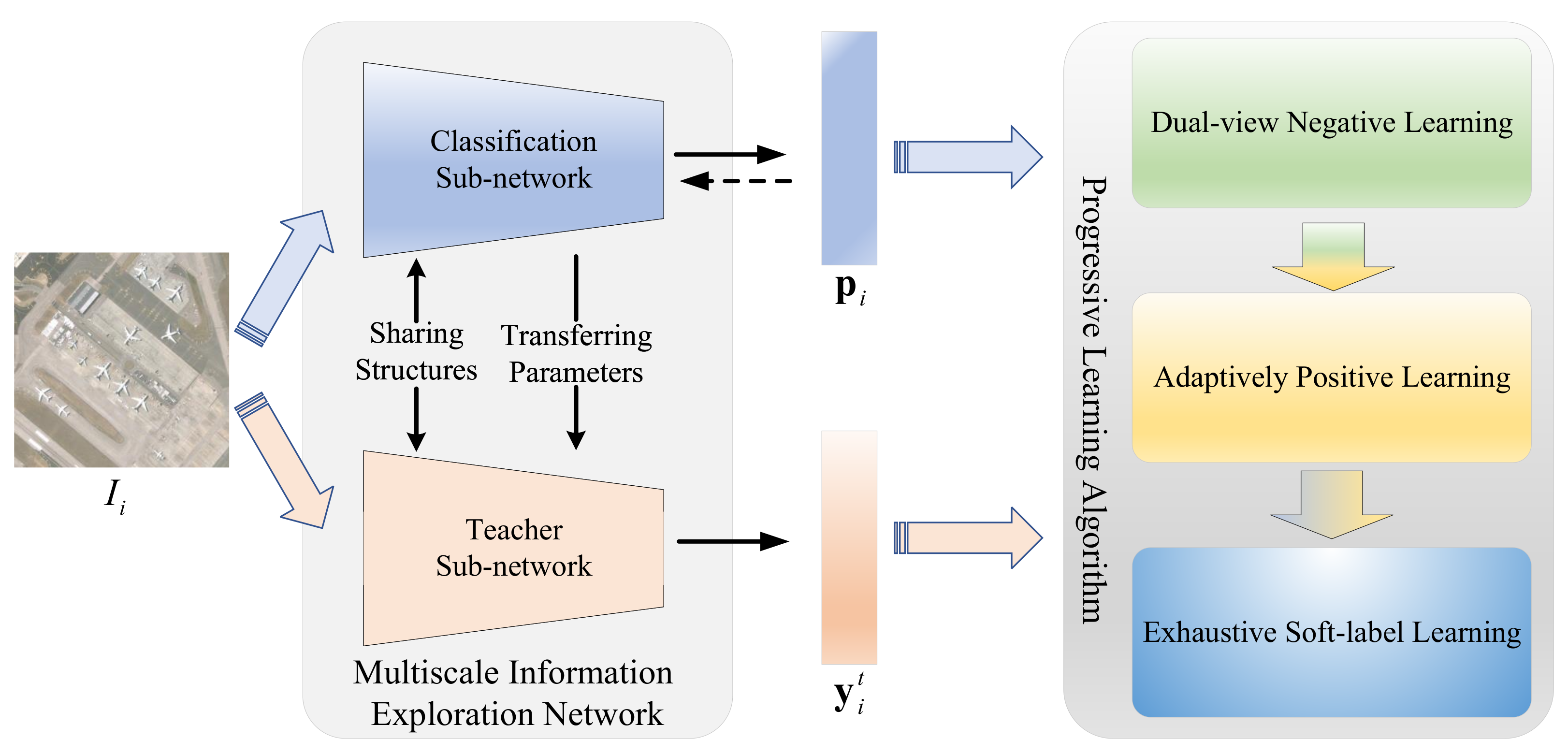
• We propose a specialized network (i.e., MIEN) and a specific learning algorithm (i.e., PLA) to effectively address the challenges posed by noisy labels in RS scene classification tasks. Combining them, not only can the significant features be mined from RS scenes, but also the adverse effects caused by noisy labels can be whittled down.
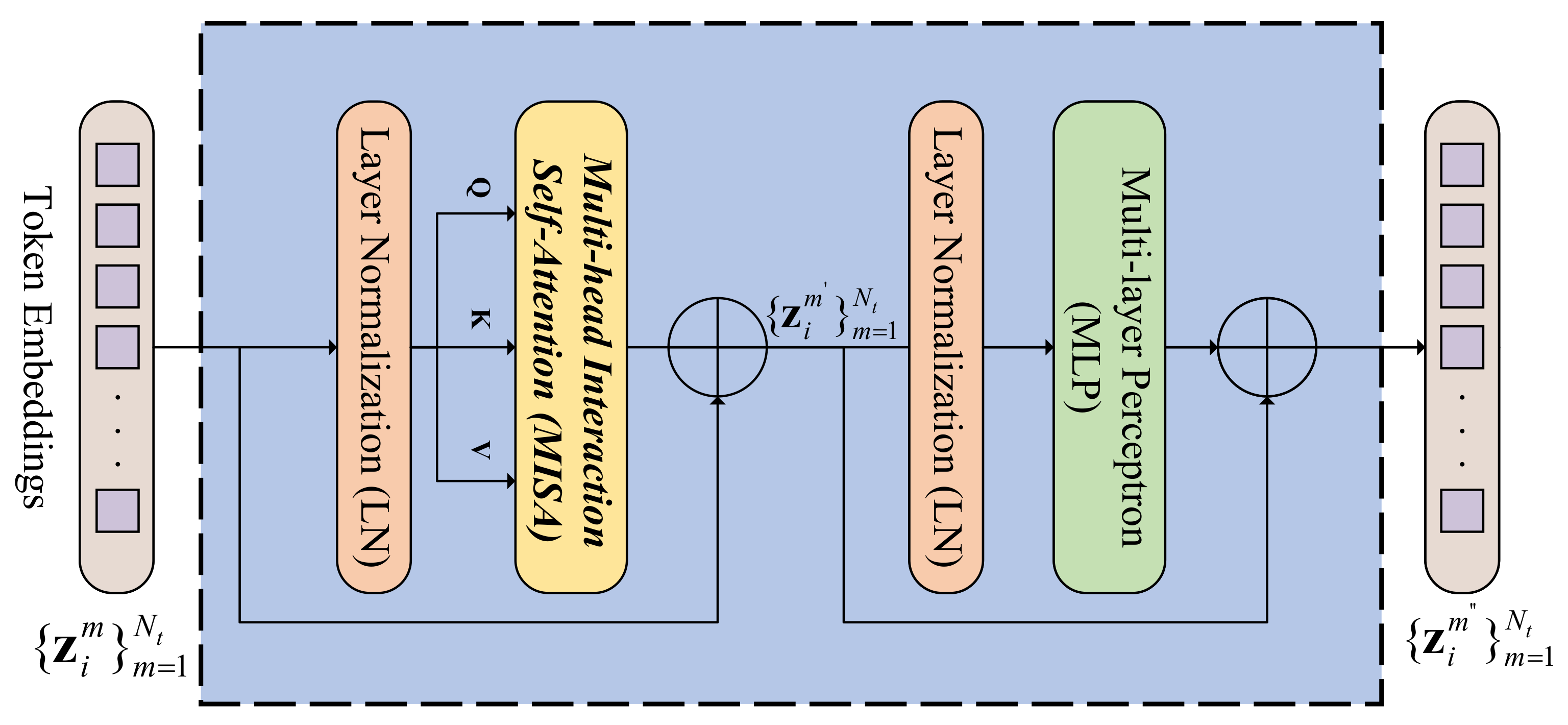
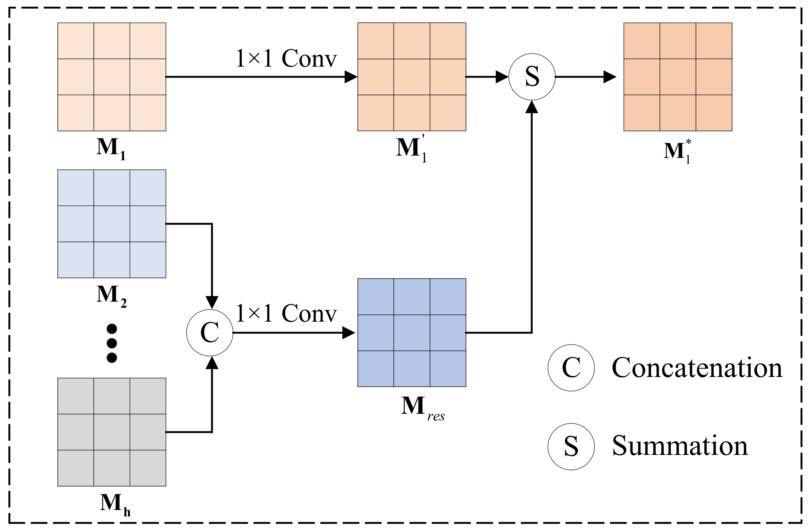
• To fully explore the contents within RS scenes, TAMSFM is developed, which fuses the different immediate features learned by ResNet18 in an interactive self-attention manner. This way, the local, multiscale, and intra-/inter-level global information hidden in RS scenes can be mined.
• MIEN is designed as a dual-branch structure to mitigate the influence of noisy samples at the network architecture level. Two branches have the same sub-networks, i.e., ResNet18 embedded with TAMSFM. MIEN can instinctively discover the possible noisy RS scenes through the different parameter updating schemes and the temporal information-aware parameter-transmitting strategy.
• PLA contains three consecutive steps, i.e., DNL, APL, and ESL, to further whittle noisy samples’ impacts and improve the classification results. After applying them to MIEN orderly, the comprehensive relations between RS scenes and their annotations can be learned. Thus, the behavior of MIEN can be guaranteed, even if some RS scenes are misannotated.

The rest of this article is organized as follows. Section 2 reviews the literature on RS scene classification methods with/without noisy labels. Then, the proposed MIEN and PLA are introduced in Section 4. Section 5 exhibits the experimental results and the related discussion. Finally, a short conclusion is drawn in Section 7.

2. Related Work

2.1. RS Scene Classification

In this section, we divide the current RS scene classification methods into two groups according to their backbone model for a short review.

Based on normal CNNs, diverse networks have been proposed and are partitioned into the first group. Considering the complicated contents within RS scenes, an attention-consistent network (ACNet) was proposed in [25]. Instead of the individual RS scene, ACNet receives the scene pairs to explore rich information using ResNet and spatial–spectral attention mechanisms. Then, an attention-consistent scheme is developed to eliminate information biases. The reported results confirm ACNet’s effectiveness in RS scene classification. A semantic-aware graph network (SAGN) was proposed in [26]. With the help of pixel features extracted by CNNs, SAGN adaptively captures object-level region features from RS scenes and establishes unstructured semantic relationships. Combining these three elements lays the foundation for SAGN’s achievements. Wang et al. [27] developed an RS scene classification model that consists of a feature pyramid network, a deep semantic embedding, and a simple feature fusion block. This model first learns the multi-layer features from RS scenes. Then, deep semantic embedding and simple feature fusion approaches are used to integrate the contributions of multi-layer features in a coarse-to-fine way. The positive results counted on different RS scene data sets demonstrate the model’s usefulness. Similarly, other CNN-based models have also been presented to explore the multiscale information from RS scenes for the final tasks, such as [28,29,30,31]. Some few-shot CNN-based models were constructed to reduce the demands for the labeled data. Tang et al. [32] proposed a dual-branch network and a corresponding class-level prototype guided learning algorithm. Based on the prototype idea, the multiscale and multi-angle clues within RS scenes can be mined from RS scenes for accurate classification results using a limited labeled sample. To compact/separate the intra-/inter-class samples, an end-to-end CNN was presented by combining contrastive learning and metric learning [33]. Along with a specific CNN and loss function, encouraging classification results can be obtained with low costs of labels. To avoid designing CNNs artificially, Peng et al. [34] introduced a neural architecture search method for RS scene classification. Inspired by the step-by-step greedy search strategy and gradient optimization algorithm, the best-fit model that is able to mine the information of RS scenes can be found.

In the second group, the methods are always transformer-based. The transformer was first developed for natural language processing [35] and has recently become increasingly fashionable for image processing [36]. Owing to the forceful capacity of capturing long-distance relations, a growing number of transformer-based methods have been proposed for various computer vision [16,17] tasks, as well as for diverse RS tasks [37,38,39]. To simultaneously mine the homogenous and heterogenous information within RS scenes, a homo-heterogenous transformer learning framework was proposed in [40]. By dividing RS scenes into regular and irregular patches, rich knowledge hidden in RS scenes can be mined by the transformer for the downstream classification task. Lv et al. [41] proposed a spatial-channel feature-preserving vision transformer (SCViT) model for RS scene classification. Based on the vanilla vision transformer, SCViT progressively aggregates the neighboring overlapping patches to deeply capture spatial information. Furthermore, it adopts a lightweight channel attention module to discover spectral messages. Combining them together, satisfying results can be generated. To further enhance the transformer’s efforts for RS scene classification, a new model named efficient multiscale transformer and cross-level attention learning (EMTCAL) was proposed in [42]. EMTCAL combines CNN and the transformer’s advantages to simultaneously extract local and global information from RS scenes. EMTCAL can understand RS scenes adequately and achieve superior classification performance by modeling the contextual relationships within and between multi-layer features. Furthermore, a novel teacher–student network was proposed with the help of the transformer in [43]. The transformer-based teacher branch focuses on contextual information, while the CNN-based student branch is aimed at local knowledge. After the knowledge distillation, this teacher–student network can achieve good performance.

2.2. RS Scene Classification with Noisy Labels

With the rapid growth of RS scene images, it is impossible to ensure that each RS scene has the correct label [44]. Therefore, developing suitable models to deal with RS scene tasks with noisy labels has attracted more and more attention [45,46,47,48]. To avoid the classification performance being seriously decreased by noisy samples in RS data sets [49], scholars have initially focused on finding and eliminating possible noises. Tu et al. [50] designed a covariance matrix representation-based noisy label model (CMR-NLD) to detect and remove noisy samples. CMR-NLD uses covariance to measure the similarity between samples in each land cover class. Then, a decision threshold is set to realize the detection and removal of noisy labels. Zhang et al. [51] proposed a noisy label distillation method based on the end-to-end teacher–student framework. Without pre-training on clean or noisy data, the teacher model effectively distills knowledge for the student model from the noisy data set so that the student model can achieve excellent results on the limited clean data set. Although the above methods are feasible, we cannot ignore the information loss caused by the elimination operation. In other words, some clean samples would be accidentally removed.

To overcome the above limitation, researchers aim to develop error-tolerant models. A simple yet effective RS-oriented error-tolerant deep learning approach was proposed in [52] for RS scene classification, where the idea of ensemble learning is introduced. By partitioning the original data set into several subsets, a group of multi-view CNNs can be learned iteratively, which are then used to distinguish the confident and unconfident samples. Then, the unconfident samples are relabeled by a support vector machine. After that, the original data set is cleaned, and the final classification results are improved. Based on [52], a more comprehensive work was published in [21]. Kang et al. [22] introduced deep metric learning to address the RS scene classification with noisy labels. First, a robust normalized softmax loss (RNSL) function is developed to help CNN learn the credit similarities between RS scenes. Then, the truncated version of RNSL (t-RNSL) is also proposed to further study the relations between inter-/intra-class samples. The reported results confirm that the obtained relationships can support the classification task, even if there are some noises. A similar work, named noise-tolerant deep neighborhood embedding (NTDNE), was published in [53]. The specific loss function is developed based on deep neighborhood embedding to guarantee that the classification model can be trained robustly. Another RS scene classification model combining ordinary learning and complementary learning (RS-COCL) is proposed in [54] to mitigate the negative influence of noisy labels. Complementary learning aims to prevent the model from learning incorrect information from noisy labels, while ordinary learning focuses on reducing the risks of overfitting. The final model can achieve favorable results under a noisy scenario through a two-stage training strategy.

3. Materials

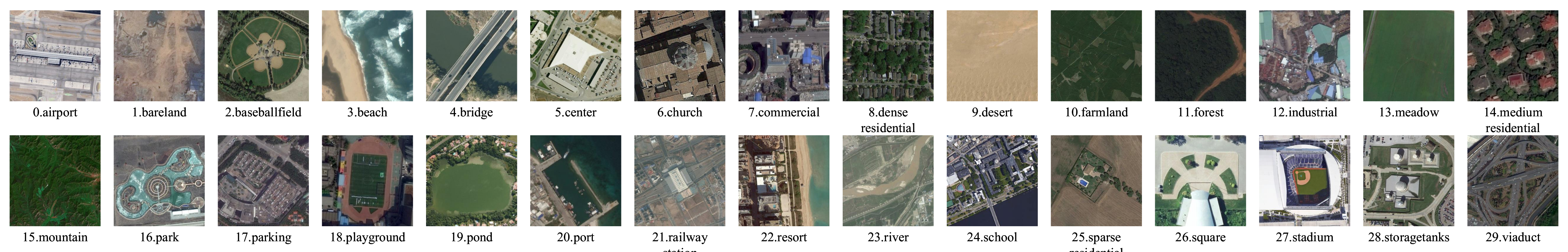
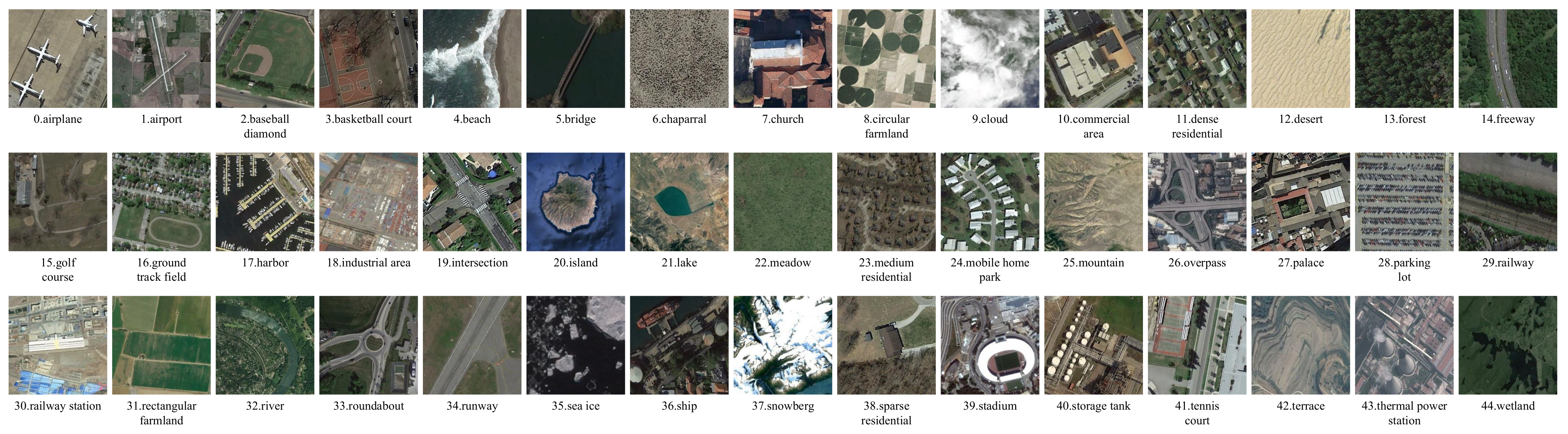
3.1. Data Set Description

In this paper, we select three RS data sets to verify the proposed method; they are the UC Merced land use data set (UCM21) [55], the aerial image data set (AID30) [56], and the Northwestern Polytechnical University (NWPU) remote-sensing image scene classification data set (NWPU45) [57]. UCM21 is a widely used RS scene data set that was published in 2010. The original RS images are provided by the United States Geological Survey (USGS), which cover 20 United States cities. After the pre-processing and manual annotation, 2100 RS scenes with $256\times 256$ pixels are selected to compose this data set. Their pixel resolution is 0.3 m, and they are divided into 21 semantic classes equally. Figure 1 shows the samples and their semantics of UCM21. The AID30 data set was constructed by Wuhan University in 2017. It contains 10,000 RS scenes with a size of $600\times 600$, and their pixel resolution ranges from 8 m to 0.5 m. These RS scenes are partitioned into 30 semantic classes, and the number of scenes in each class varies from 220 to 420. The properties of multi-resolution and class imbalance enhance the difficulties in understanding AID30. The examples of different classes of AID30 are displayed in Figure 2. NWPU45 is a large-scale RS scene data set, which encloses 31,500 scenes that are equally distributed in 45 semantic categories. The sizes of these scenes are $256\times 256$, and their minimum and maximum pixel resolutions are 0.2 m and 30 m, respectively. The examples and the corresponding semantics are exhibited in Figure 3.

3.2. Evaluation Metrics

The overall accuracy (OA) is used to evaluate the effectiveness of our MIEN and PLA numerically. OA is the number of correctly classified samples divided by the total number of testing samples. Apart from OA, the confusion matrix (CM) is also chosen to further observe the classification results across the different categories. The row of CM represents the ground truths, while the column represents the predictions.

4. Proposed Method

4.1. Preliminaries

Before introducing the proposed method, some notations are first defined here. We use $\mathcal{D}={\left\{(I_i,y_i)\right\}}_{i=1}^N$ to represent an RS scene data set, where $I_i\in \mathcal{I}$ indicates the i-th RS scene, $y_i\in \mathcal{Y}$ denotes the corresponding manual label, and N implies the volume of this data set. Note that the data set has c classes, i.e., $\mathcal{Y}=\{1,\dots ,c\}$. Generally speaking, we believe the manual labels’ correctness. However, some RS images are misannotated due to complicated and uncontrollable factors. To represent this situation, we assume that there is a set of ground truths, ${\mathcal{Y}}^{*}=\{1,\dots ,c\}$, and each RS image, $x_i$, has a ground truth, $y_i^{*}$. When $y_i\ne y_i^{*}$, the sample $I_i$ will be regarded as noisy data. A range of networks [58,59] has been proposed to deal with RS scene classification. However, they do not take the noisy data into account. Thus, their behavior would be whittled sharply when RS scenes have incorrect manual labels. To mitigate this problem, we construct an MIEN. By adopting the teacher–student paradigm, our MIEN can handle the RS scene classification under the noisy scenario.

The most widely used loss function for supervised RS scene classification is the cross-entropy (CE) loss function [26,60], and its formulation is

$${\mathcal{L}}_{CE}(g(x_i;\theta ),y_i)=-\sum _{k=1}^c{\mathbf{y}}_i^{k}log{\mathbf{p}}_i^k,$$

(1)

where $g\left(·\right)$ refers to the classification model with the parameters of $\theta$, ${\mathbf{y}}_i^k\in {\left\{0,1\right\}}^c$ is a one-hot vector of $y_i$, and ${\mathbf{p}}_i^k\in {\left[0,1\right]}^c$ is a probability vector, which is obtained by the classification model and the softmax function. Here, the dimensions of ${\mathbf{y}}_i^k$ and ${\mathbf{p}}_i^k$ are c. The k-th element of ${\mathbf{y}}_i^k$ equals 1, and the others are 0. The k-th element of ${\mathbf{p}}_i^k$ has the largest value among all elements. Numerous works (e.g., [26,60]) confirm the usefulness of the CE loss in RS scene classification. Nevertheless, the precondition is that all RS scenes are labeled correctly. In the noisy scenario, its performance cannot reach what we expected. Thus, specific training strategies should be added to ensure the classification results. Considering this, we developed the progressive learning algorithm in this paper to guarantee that the CE loss can be worked smoothly for noisy cases.

4.2. Multiscale Information Exploration Network

The overall framework of the proposed method is shown in Figure 4, which mainly contains MIEN and PLA. In the training phase, the input RS scene is first mapped into a probability vector, $\mathbf{p}$, and a prediction label vector, ${\mathbf{y}}^t$, by MIEN. Then, PLA is applied to them to optimize MIEN. When the model is trained, we only use the probability vector, $\mathbf{p}$, to complete the classification. In this section, we will introduce MIEN in detail. As shown in Figure 4, our MIEN has two identical sub-networks, i.e., a classification sub-network and a teacher sub-network. The former is responsible for learning sufficient information and completing the classification task, and the latter integrates the knowledge learned by the classification sub-network to assist against noisy samples. Thus, their parameter initialization and updating schemes are different.

4.2.1. Classification Sub-Network

The architecture of the classification sub-network is shown in Figure 5. Its backbone is ResNet18, which contains four residual modules. When an RS scene, $I_i$, is input into the classification sub-network, it is mapped into feature maps ${\mathbf{B}}_i^1\in {\mathbb{R}}^{H_1\times W_1\times C_1}$, ${\mathbf{B}}_i^2\in {\mathbb{R}}^{H_2\times W_2\times C_2}$, ${\mathbf{B}}_i^3\in {\mathbb{R}}^{H_3\times W_3\times C_3}$, and ${\mathbf{B}}_i^4\in {\mathbb{R}}^{H_4\times W_4\times C_4}$ by different residual modules, where $H_l$, $W_l$, and $C_l$ represent the height, width, and the number of channels of the l-th feature map ($1\le l\le 4$). Customarily, the global feature vector, ${\mathbf{g}}_i^{res}\in {\mathbb{R}}^{C_4}$, can be produced by ${\mathbf{B}}_i^4$ for the downstream tasks through average pooling. However, since the contents within RS scenes are diverse in type and abundant in volume, the valuable and multiscale messages within the first three feature maps (i.e., ${\mathbf{B}}_i^1$, ${\mathbf{B}}_i^2$, and ${\mathbf{B}}_i^3$) should be considered at the same time to guarantee the discrimination of the final global vector. The common solutions for this target are simple concatenation and pixel-wise addition. Although feasible, they ignore the global contextual information within and across the different feature maps, which prevents the model from understanding RS scene images [61,62]. Therefore, we developed TAMSFM to deeply mine and integrate the useful information hidden in different feature maps.

The flowchart of TAMSFM is also exhibited in Figure 5. First, we apply three $1\times 1$ convolutions to ${\mathbf{B}}_i^1$, ${\mathbf{B}}_i^2$, and ${\mathbf{B}}_i^3$ for unifying their channels into $C_4$. Then, three average pooling operations are used to adjust their spatial sizes to $H_4\times W_4$. After the above two steps, we can obtain ${\mathbf{B}}_i^{1*}\in {\mathbb{R}}^{H_4\times W_4\times C_4}$, ${\mathbf{B}}_i^{2*}\in {\mathbb{R}}^{H_4\times W_4\times C_4}$, and ${\mathbf{B}}_i^{3*}\in {\mathbb{R}}^{H_4\times W_4\times C_4}$. Next, ${\mathbf{B}}_i^{1*}$, ${\mathbf{B}}_i^{2*}$, ${\mathbf{B}}_i^{3*}$, and ${\mathbf{B}}_i^4$ are normalized by L2 norms and spliced into a feature matrix ${\mathbf{X}}_i\in {\mathbb{R}}^{2H_4\times 2W_4\times C_4}$ orderly. The obtained ${\mathbf{X}}_i$ contains rich information with various scales. To comprehensively understand those significant clues for classification, we developed a cross-head information interaction transformer (CIIT) encoder, whose structure is exhibited in Figure 6. Note that there are $N_t$ CIIT encoders in TAMSFM.

Like the standard vision transformer (ViT) [36], our CIIT encoder includes a multi-head interaction self-attention (MISA) block and a multi-layer perception (MLP) block (encompassing two fully connected layers and a Gaussian error linear unit). In addition, the layer normalization (LN) operation exists before each block. Two blocks are connected in a residual way. For the input, ${\mathbf{X}}_i$, the first CIIT encoder’s process can be formulated as

$$\begin{array}{c}{\mathbf{z}}_i^1=\mathrm{embed}\left({\mathbf{X}}_i\right),\\ \mathbf{z}{{}_i^1}^{{}^{\prime }}={\mathbf{z}}_i^1+\mathrm{MISA}\left(LN\left({\mathbf{z}}_i^1\right)\right),\\ \mathbf{z}{{}_i^1}^{{}^{\prime \prime }}=\mathbf{z}{{}_i^1}^{{}^{\prime }}+MLP\left(LN\left(\mathbf{z}{{}_i^1}^{{}^{\prime }}\right)\right),\end{array}$$

(2)

where $embed\left(·\right)$, $LN\left(·\right)$, $MISA\left(·\right)$, and $MLP\left(·\right)$ indicate the embedding LN, MISA, and MLP functions and ${\mathbf{z}}_i^1$, $\mathbf{z}{{}_i^1}^{{}^{\prime }}$, and $\mathbf{z}{{}_i^1}^{{}^{\prime \prime }}$ are the token embeddings of ${\mathbf{X}}_i$ and the outputs of the MISA and MLP blocks in the first CIIT encoder. This way, the obtained $\mathbf{z}{{}_i^1}^{{}^{\prime \prime }}$ are rich in both the multiscale information and the inter- and intra-level relations, which are beneficial to the following classification tasks. Furthermore, $\mathbf{z}{{}_i^1}^{{}^{\prime \prime }}$ can be regarded as the input embeddings of the next CIIT encoder. In a similar fashion, we can obtain the multiscale feature vector, ${\mathbf{g}}_i^{*}\in {\mathbb{R}}^{C_4}$, after the $N_t$ CIIT encoders with the average pooling and reshaping operations.

When we obtain ${\mathbf{g}}_i^{*}$, it is concatenated with the global feature ${\mathbf{g}}_i^{res}$ at the channel dimension to generate mixed feature ${\mathbf{g}}_i$, which encloses multiscale and high-level semantic knowledge. After a fully connected layer, the probability vector, ${\mathbf{p}}_i$, can be obtained. In the training phase, the parameters of the classification sub-network are updated according to the gradient back propagated by the proposed progressive learning algorithm.

We will now further explain the MISA block. MISA is developed based on the multi-head self-attention (MSA) mechanism. For clarity, we first explain MSA briefly, whose structure is shown in Figure 7a. For the general token embeddings, $\mathbf{Z}$, the process of MSA is defined as

$$\begin{array}{c}MSA\left(\mathbf{Z}\right)=Concat\left(hea{d}_1,\cdots ,hea{d}_h\right){\mathbf{W}}^O,\\ hea{d}_j=\mathrm{Att}\left(\mathbf{Z}{\mathbf{W}}_j^Q,\mathbf{Z}{\mathbf{W}}_j^K,\mathbf{Z}{\mathbf{W}}_j^V\right),\\ Att\left(\mathbf{Q},\mathbf{K},\mathbf{V}\right)=softmax\left(\mathbf{M}/\sqrt{d_k}\right)\mathbf{V},\mathbf{M}=\mathbf{Q}{\mathbf{K}}^T,\end{array}$$

(3)

where $MSA\left(·\right)$, $Concat\left(·\right)$, $Att\left(·\right)$, and $softmax\left(·\right)$ indicate the functions of MSA, concatenation, self-attention, and softmax; h represents the number of self-attention heads; $hea{d}_j$ implies the j-th self-attention head; ${\mathbf{W}}^O$, ${\mathbf{W}}_j^Q$, ${\mathbf{W}}_j^K$, and ${\mathbf{W}}_j^V$ denote learnable parameter matrices; $\mathbf{M}$ refers to the intermediate attention maps; and $\sqrt{d_k}$ expresses a scaling factor. According to the above explanation, MSA first divides the original token embeddings into distinct projection spaces and then analyzes the global relations within different spaces. After combining various global relations, the attention relationships of embeddings can be obtained. This way is feasible. However, the knowledge within each space is inadequate, which limits MSA’s performance in capturing the long-range relationships hidden in the input data. Especially for RS scenes, only using the partial information from projection spaces cannot generate the proper global relationships among the complex contents.

In the face of such a challenge, we developed MISA, and its structure is exhibited in Figure 7b. MISA aims to enhance the capability of information acquisition by considering the mutual influence of different projection spaces. In this fashion, both the messages within projection spaces and the clues between projection spaces can be explored, which facilitates the comprehensive acquisition of complex contents from RS scenes. First, we map the token embeddings, $\mathbf{Z}$, into ${\left\{({\mathbf{Q}}_i,{\mathbf{K}}_i,{\mathbf{V}}_i)\right\}}_{i=1}^h$ and produce attention maps, ${\left\{{\mathbf{M}}_i\right\}}_{i=1}^h$, according to Equation (3). Next, instead of directly multiplying ${\mathbf{M}}_i$ by ${\mathbf{V}}_i$, we design a cross-head associating module (CAM) to capture the mutual clues between various projection spaces and achieve the enhanced attention maps, ${\left\{{\mathbf{M}}_i^{*}\right\}}_{i=1}^h$. Since CAM operates in the same way for different ${\mathbf{M}}_i$, we explain its working process using ${\mathbf{M}}_1$ as an example. As shown in Figure 8, a $1\times 1$ convolution is first applied on ${\mathbf{M}}_1$ to generate ${\mathbf{M}}_1^{{}^{\prime }}$. By doing so, the risk of different ${\left\{{\mathbf{M}}_i\right\}}_{i=1}^h$ converging will be reduced. Meanwhile, a concatenation and a $1\times 1$ convolution is applied to the remaining attention maps, ${\left\{{\mathbf{M}}_i\right\}}_{i=2}^h$, to generate ${\mathbf{M}}_{res}$. The concatenation combines the messages from diverse projection spaces, while the $1\times 1$ convolution reduces the dimensions. Then, the integrated attention map, ${\mathbf{M}}_{res}$, will be fused with ${\mathbf{M}}_1^{{}^{\prime }}$ by a simple summation. The above process can be formulated as

$$\begin{array}{c}{\mathbf{M}}_1^{*}=\mathrm{CAM}({\mathbf{M}}_1,\dots ,{\mathbf{M}}_h,i),i=1,\\ \mathrm{CAM}({\mathbf{M}}_1,\dots ,{\mathbf{M}}_h,i)=\mathrm{co}{\mathrm{n}}_{1\times 1}\left({\mathbf{M}}_i\right)+{\mathbf{M}}_{res},\\ {\mathbf{M}}_{res}=\mathrm{co}{\mathrm{n}}_{1\times 1}(\mathrm{Concat}({\mathbf{M}}_1,\dots ,{\mathbf{M}}_{i-1},{\mathbf{M}}_{i+1},\dots ,{\mathbf{M}}_h)),\end{array}$$

(4)

where $CAM\left(·\right)$ indicates the CAM function. When we obtain the enhanced attention maps, ${\left\{{\mathbf{M}}_i^{*}\right\}}_{i=1}^h$, they will be multiplied by ${\left\{{\mathbf{V}}_i\right\}}_{i=1}^h$ to continue the self-attention operations. In addition, since CAM is independent for different ${\mathbf{M}}_i$, this ensures the difference of information in different projection spaces, facilitating the capture of diverse levels and aspects of information within RS scenes.

4.2.2. Teacher Sub-Network

In general, the above classification sub-network is able to handle the common RS scene classification tasks. Nonetheless, when there are some noisy samples (i.e., the RS scenes with incorrect labels), the classification sub-network would be out of work since the cumulative errors generated by noisy samples have a severe negative effect [63,64,65]. To overcome this problem, we introduce a teacher sub-network inspired by [66]. It leverages the temporal process information from the classification sub-network to make diverse predictions under the noisy scenario. These diverse predictions can help the classification sub-network recognize the noisy samples along with our PLA.

Particularly, the teacher sub-network has an identical structure to the classification sub-network, and its output probability vector is ${\mathbf{y}}_i^t$ (for RS scene $I_i$). To accomplish the prediction without increasing the training complexities, the weights of the teacher sub-network are inherited from the classification sub-network temporally, i.e.,

$${\theta }_s^t=\alpha {\theta }_{s-1}^t+\left(1-\alpha \right){\theta }_s^c,$$

(5)

where ${\theta }_s^t$ and ${\theta }_s^c$ represent the teacher and classification sub-networks’ parameters at the s-th training step, ${\theta }_{s-1}^t$ denotes the teacher sub-network’s parameters at the $\left(s-1\right)$-th training step, and $\alpha$ is a hyper-parameter to smooth this transition. Note that the initial parameters of the teacher sub-network are replicated from the classification sub-network. In this fashion, the predictions of the teacher sub-network contain both the knowledge learned in the current state (transmitted from the classification network) and the information discovered in the previous states. Therefore, these predictions may differ from the outputs of the classification sub-network, which would be caused by the noisy samples. By investigating these different clues, the adverse impacts of noisy samples on the classification sub-network can be weakened.

4.3. Progressive Learning Algorithm

The developed PLA consists of three stages, i.e., the DNL, APL, and ESL stages. In the DNL stage, our MIEN focuses on learning the valuable information hidden in RS scenes indirectly, i.e., modeling the relationships between RS scenes and irrelevant categories. In the APL stage, MIEN aims to discover profitable knowledge by selecting credible RS scenes and creating links between them and their corresponding semantic categories. After the above two stages, our MIEN has the primary capacity to distinguish between the clean and noisy samples. Therefore, the entire RS scenes within the data set will be relabeled, and all of the scenes and their pseudo-labels will be adopted to train MIEN in the ESL stage.

4.3.1. Dual-View Negative-Learning Stage

Directly bridging the relationships between RS scenes and their semantic labels is a common training method for CNNs. Unfortunately, it is disabled when there are noisy samples, as incorrect relations prevent CNNs from exploring useful information. To alleviate this problem, an alternative method is to learn the irrelevant links [67]. In short, the deep neural networks can be trained using the messages that RS scenes do not belong to some categories rather than belonging to specific categories under the noisy scenario. For instance, for an RS scene and its manual label, $\left\{I_i,y_i\right\}$, the following clue, $I_i$ does not belong to ${\overline{y}}_i$, is always correct, regardless of whether $y_i\ne y_i^{*}$ or $y_i=y_i^{*}$. Here, ${\overline{y}}_i$ indicates a complementary label within $\mathcal{Y}$ other than $y_i$, and $y_i^{*}$ is the ground truth of $I_i$. Using these clues to train CNNs can reduce the risks caused by noisy labels. With the help of this idea, we developed the DNL stage in this section.

First, a dual-view complementary label selection strategy is developed. The complementary label means a label other than the manual annotation and ground truth. Considering the complex contents of RS scenes, both the manual labels and the predictions from the teacher sub-network are used to decide the complementary labels. Specifically, for a given RS scene, $I_i$, suppose that the manual label and the teacher sub-network’s prediction label are $y_i$ and $y_i^t$. The complementary label ${\overline{y}}_i$ can be randomly selected from a subset of $\mathcal{Y}$ that does not contain $y_i$ and $y_i^t$. This step is formulated as

$${\overline{y}}_i=\mathrm{Randomly}\mathrm{select}\{1,\dots ,c\}\setminus \{y_i,y_i^t\}.$$

(6)

If $I_i$ is a clean sample, the above label selection strategy ensures the complementary label is irrelevant to $I_i$. If $I_i$ is a noisy sample, the combination of $y_i$ and $y_i^t$ can also support the label selection strategy to find an irrelevant label.

Then, the negative-learning (NL) loss function [67] is introduced to train the classification sub-network using the irrelevant scene and label pairs. Its definition is

$${\mathcal{L}}_{NL}(g_{cls}(I_i;{\theta }_{cls}),{\overline{y}}_i)=-\sum _{k=1}^c{\overline{\mathbf{y}}}_i^{k}log(1-{\mathbf{p}}_i^k),$$

(7)

where $g_{cls}\left(·\right)$ denotes the classification sub-network with the parameters ${\theta }_{cls}$, ${\overline{\mathbf{y}}}_i^k\in {\left\{0,1\right\}}^c$ is the one-hot vector of ${\overline{y}}_i$, and ${\mathbf{p}}_i^k$ is the classification sub-network’s prediction. By applying the NL loss function, our MIEN can learn that RS scenes do not belong to certain categories. Correspondingly, the relations between RS scenes and their “true” labels can be explored.

4.3.2. Adaptively Positive-Learning Stage

After the DNL stage, MIEN can distinguish the RS scenes not belonging to certain categories. Now, we want to connect RS scenes and their “true” labels. To achieve this, we first design an adaptive clean sample selection scheme. For an RS scene, $I_i$, suppose its manual label and two sub-networks’ predictions are $y_i$, $y_i^c$, and $y_i^t$. If $y_i=y_i^c=y_i^t$, $I_i$ can be regarded as a clean sample and otherwise as a noisy sample. The reasonableness of this simple rule is summarized as follows: First, compared to the noisy samples, the clean samples are easier to fit by the common deep networks [20,68]. Therefore, if $y_i=y_i^c$, the scene’s probability of a clean sample is higher. Second, as mentioned in Section 4.2.2, the target of the teacher sub-network is to help MIEN discover the noisy samples by analyzing the temporal information. The output of the teacher sub-network can be regarded as the average result of the classification sub-network within the past periods. The different outputs indicate the fluctuations in the fitting process, which may be generated by noisy samples. Hence, if their outputs are consistent (i.e., $y_i^c=y_i^t$), $I_i$ is more likely to be a clean sample. To sum up, we can decide whether $I_i$ is clean in line with $y_i=y_i^c=y_i^t$.

Based on the above selection scheme, we can collect a clean subset, ${\mathcal{D}}_{sub}={\left\{(I_i,y_i)\right|y_i=y_i^c=y_i^t\}}_{i=1}^{N_{sub}}$, adaptively, where $N_{sub}$ implies the number of scenes contained in the subset. Then, the CE loss can be applied to ${\mathcal{D}}_{sub}$ to train our MIEN, and it is formulated as

$${\mathcal{L}}_{CE}^{APL}(g_{cls}(I_i\in D_{sub};{\theta }_{cls}),y_i)=-\sum _{k=1}^c{\mathbf{y}}_i^{k}log{\mathbf{p}}_i^k.$$

(8)

Once the APL stage is completed, the relationships between clean RS scenes and their labels are established, while the noisy RS scenes can be ignored.

4.3.3. Exhaustive Soft-Label Learning

After the DNL and APL stages, the negative and positive relationships between RS scenes and the corresponding semantics are partially explored. To further and comprehensively mine the valuable information hidden in RS scenes, we developed the ESL stage at the end of the progressive learning algorithm.

In contrast to the above two learning stages, which leverage partial labels or RS scenes to complete the information extraction, we need whole scenes to be considered. For this purpose, all RS scenes should be relabeled according to the obtained knowledge. Therefore, a label reassignment strategy is designed. For an RS scene, $I_i$, we generate its soft pseudo label ${\tilde{\mathbf{y}}}_i$ vector by combining its own one-hot label vector ${\mathbf{y}}_i$ and the prediction of the teacher sub-network ${\mathbf{y}}_i^t$, i.e.,

$${\tilde{\mathbf{y}}}_i=p_{y_i}\times {\mathbf{y}}_i+(1-p_{y_i})\times {\mathbf{y}}_i^t,$$

(9)

where $p_{y_i}$ represents the probability of $I_i$ belonging to class $y_i$. Here, $p_{y_i}$ is generated by the classification sub-network, whose value equals the $y_i$-th element of ${\mathbf{p}}_i$. This probability reflects whether the relationship between $I_i$ and semantic class $y_i$ is fully learned, and we can use it to express the credibility of the corresponding relation between $I_i$ and $y_i$. If the value of $p_{y_i}$ is close to 1, the link between $I_i$ and $y_i$ is strong, so the possibility of $I_i$ belonging to $y_i$ is high. Thus, the pseudo-label depends more on its label, ${\mathbf{y}}_i$, and the teacher sub-network’s output, ${\mathbf{y}}_i^t$, can be regarded as the label smoothing term [69]. If the value of $p_{y_i}$ is close to 0, the relation between $I_i$ and $y_i$ is weak. In other words, $I_i$ may not belong to $y_i$. Hence, the pseudo-label, ${\tilde{\mathbf{y}}}_i$, leans towards the output of the teacher sub-network, ${\mathbf{y}}_i^t$. Due to the variation of $p_{y_i}$, the generated pseudo-labels are highly representative and can provide unique information for different RS scenes. Once all RS scenes are re-labeled, MIEN can be trained by the CE loss using the scenes and their soft pseudo labels, i.e.,

$$L_{CE}^{ESL}(g_{cls}(I_i;{\theta }_{cls}),{\tilde{\mathbf{y}}}_i)=-\sum _{k=1}^c{{\tilde{\mathbf{y}}}_i}^{k}log{\mathbf{p}}_i^k.$$

(10)

After the ESL stage, the whole information of the RS scene data set can be thoroughly mined. Consequently, the classification results’ accuracy can be ensured under the noisy scenario.

5. Results

5.1. Experiment Settings

The following experiments are conducted on an NVIDIA TITAN Xp with 12 GB Memory, from ASUS Xi’an, China, using the Pytorch 1.9.0 [70] platform. The reported results are the average values of the five random trials. We divide three data sets into the training and testing sets randomly according to [40,41,42]. The ratios of the training and testing sets are 8:2 (UCM21), 5:5 (AID30), and 2:8 (NWPU45). All RS scenes are resized into $224\times 224$ for MIEN, and the common data augmentation strategies (e.g., random horizontal/vertical flip, normalization, label smooth) are adopted to ensure the stability of the training process.

The ResNet18 part of our MIEN is initialized by the pre-trained parameters obtained on the ImageNet data set [71], and the other parts are initialized randomly. Before training MIEN using the proposed PLA, it is warmed up for two epochs using the normal CE loss. In the formal training stage, the batch size is 64 for the three data sets. However, the epochs are different for them. In detail, the training epochs equal 90 for UCM21, with 40 for the DNL stage, 25 for the APL stage, and 25 for the ESL stage. For AID30 and NWPU45, the training epochs are equal to 150, with 50 for the DNL stage, 50 for the APL stage, and 50 for the ESL stage. The SGD optimizer with an initial learning rate of 0.005 and a momentum of 0.9 is adopted to optimize the parameters of MIEN. Note that the learning rate would be reduced by half every 5 (UCM21)/10 (AID30 and NWPU45) epochs in the last 15 (UCM21)/30 (AID30 and NWPU45) epochs. Three free parameters are decided in advance, i.e., the smooth transition weight, $\alpha$ (Equation (5)), the head number in MISA, h, and the number of the CIIT encoder, $N_t$. For $\alpha$ and $N_t$, we fix them to be 0.99 and 1. The value of h equals 2 for UCM21 and AID30 and equals 4 for NWPU45. Their influence on our MIEN and APL will be discussed in Section 5.4.

Generally speaking, there are two popular types of noisy label [72]: symmetric and asymmetric. The symmetric noisy labels mean that the researchers randomly change the original labels of RS scenes to other categories with equal probability. The asymmetric noisy labels are obtained by flipping the original labels of the data set into similar scenes. In our experiments, we add the symmetric noisy labels into the training sets to simulate the noisy scenario. Particularly, we use a symmetric corrosion matrix [72] to randomly replace a certain percentage of RS scenes’ labels with other categories for establishing the noisy scenario. The mentioned percentage is recorded as noise rate ($NR$).

5.2. Comparison with Existing Methods

We select nine popular noisy label classification methods to assess the performance of MIEN and PLA. There are five successful models proposed in the natural image field (SCE [73], NCE [74], RCE [73], Mixup [75], NLNL [67]) and four rewarding approaches introduced in the RS community (CMR-NLD [50], t-RNSL [22], NTDNE [53], RS-COCL [54]). All of them are completed by ourselves using the released codes. Their free parameters are set according to the original literature. For the sake of fairness, the experimental settings of the compared methods are consistent with ours, and the same backbone (ResNet18) is used in all methods. In the following experiments, we gradually increase the noise rate ($NR$) of the training set from 0.1 to 0.4 to deeply study various methods’ performances. Note that, for convenience, we record our methods as Res-PLA and MIEN-PLA in the subsequent experimental analysis. The former uses the basic ResNet18 as the classification sub-network and the teacher sub-network, and the latter replaces the backbones with our MIEN.

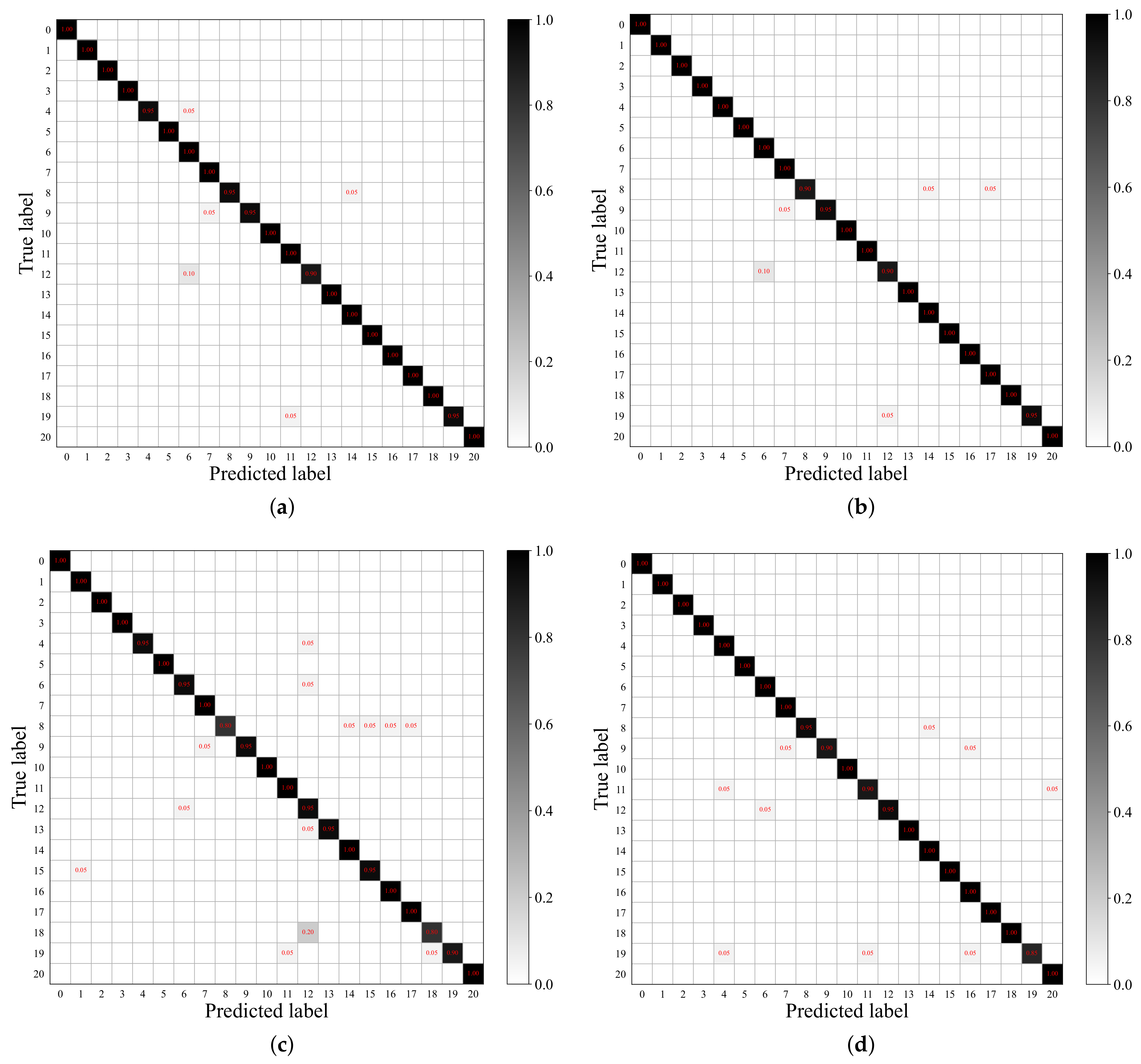
5.2.1. Results on UCM21

The OA values of different methods counted on UCM21 are shown in

Table 1. OA values (%) of different methods on UCM21 with different noise rates. The best values are marked in bold.

NR	SCE [73]	NCE [74]	RCE [73]	Mixup [75]	NLNL [67]	CMR-NLD [50]	t-RNSL [22]	NTDNE [53]	RS-COCL [54]	Res-PLA (Ours)	MIEN-PLA (Ours)
0.1	94.47	93.80	97.18	93.80	97.19	90.23	96.19	96.00	98.19	98.33	98.81
0.2	91.32	90.95	95.99	88.42	96.42	89.09	95.82	95.66	97.09	97.62	98.42
0.3	83.56	83.57	93.67	81.47	95.33	88.80	94.52	94.37	96.19	96.99	97.42
0.4	75.37	75.80	87.18	73.76	94.52	88.57	91.14	91.04	95.90	96.19	96.80

. By observation, we can see the following points: First, the weakest model is CMR-NLD. This is because it focuses on filtering the noisy samples and ignores mining the complex information hidden in RS scenes. Although the noisy sample selection scheme is applicable, the imperfect feature representation limits its performance in the noisy RS classification. Second, the performance of most models proposed for natural images (i.e., SCE, NCE, and Mixup) is lower than that of most models developed for RS scenes (i.e., t-RNSL, NTDNE, and RS-COCL). The main reason behind this is that the models in the natural field are not good at capturing the complex contents within RS scenes. Hence, their behavior cannot reach what we expected for RS cases. The fact that the distinct performance drops with the increasing $NR$ (more than ten percent) confirm this point again. In contrast to SCE, NCE, and Mixup, the three RS models’ performance declines (when $NR$ raises from 0.1 to 0.4), but not dramatically. The performance gaps are approximately five percent. Third, although t-RNSL, NTDNE, and RS-COCL have achieved good results, their behavior is weaker than Res-PLA. This implies the usefulness of the proposed noise-tolerant learning algorithm. Furthermore, when MIEN is introduced, MIEN-PLA performs best in all cases. Taking $NR=0.1$ as an example, compared with the other nine models, the OA improvements achieved by our PLA are 4.34% (over SCE), 5.01% (over NCE), 1.63% (over RCE), 5.01% (over Mixup), 1.14% (over NLNL), 8.58% (over CMR-NLD), 2.62% (over t-RNSL), 2.81% (over NTDNE), 0.62% (over RS-COCL), and 0.48% (over Res-PLA). Another encouraging observation is that our MIEN-PLA can still work well when $NR=0.4$. Its performance gap between $NR=0.1$ and $NR=0.4$ is as small as 2.01%, which is superior to other models. The positive observations discussed above demonstrate that our MIEN is helpful in noisy classification tasks for UCM21.

Apart from OA values, we also draw the CMs of MIEN-PLA at different noise rates, as shown in Figure 9. When the noise rates are low (i.e., $NR=0.1$ and $NR=0.2$), our method can predict most categories correctly. The incorrect predictions only appear in a few semantic classes, such as “freeway”, “golfcourse”, “medium residential”, and “storage tanks”. When the noise rates increase, inaccurate predictions appear in more classes. Fortunately, their error rates are in an acceptable range. These findings again illustrate the effectiveness of MIEN-PLA.

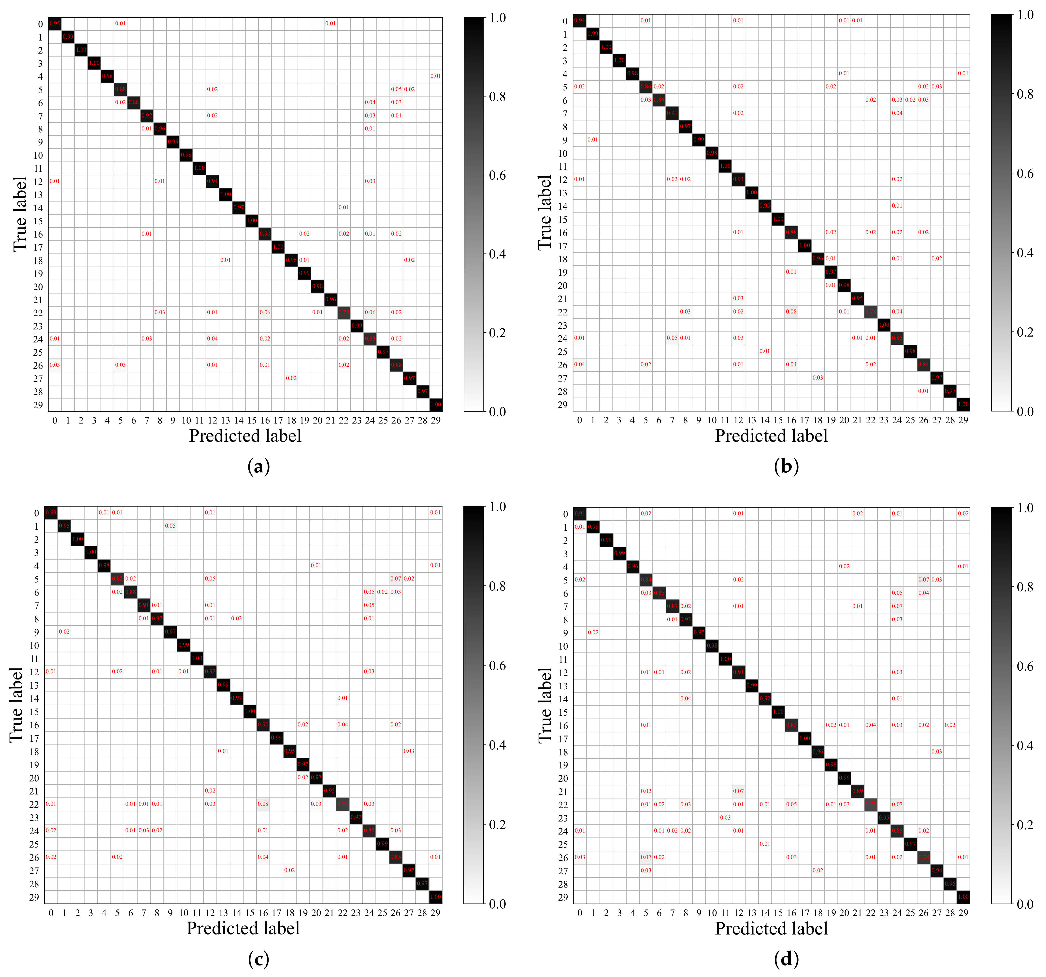
5.2.2. Results on AID30

The diverse experimental results counted on AID30 are exhibited in

Table 2. OA values (%) of different methods on AID30 with different noise rates. The best values are marked in bold.

NR	SCE [73]	NCE [74]	RCE [73]	Mixup [75]	NLNL [67]	CMR-NLD [50]	t-RNSL [22]	NTDNE [53]	RS-COCL [54]	Res-PLA (Ours)	MIEN-PLA (Ours)
0.1	91.36	91.39	94.95	92.13	94.34	85.10	95.01	94.77	95.09	95.22	95.72
0.2	86.66	86.82	93.62	89.56	93.58	84.09	94.52	94.31	94.53	95.14	95.27
0.3	78.48	78.58	91.07	82.27	92.54	83.05	92.69	92.66	94.00	94.74	94.81
0.4	71.07	70.99	88.23	77.79	91.48	82.04	91.30	91.04	93.11	93.36	93.44

. Like the conclusions of UCM21, most RS-oriented models (except CMR-NLD) outperform the natural image-oriented approaches, and our MIEN-PLA achieves the best performance among all models. Furthermore, our advantages become more prominent as $NR$ increases. Particularly, when $NR=0.1$, the improvements achieved by MIEN-PLA are 4.36% (over SCE), 4.33% (over NCE), 0.77% (over RCE), 3.59% (over Mixup), 1.37% (over NLNL), 10.62% (over CMR-NLD), 0.71% (over t-RNSL), 0.95% (over NTDNE), 0.63% (over RS-COCL), and 0.50% (over Res-PLA). When $NR$ increases to 0.4, the enhancements of MIEN-PLA are 22.37% (over SCE), 22.45% (over NCE), 5.21% (over RCE), 15.65% (over Mixup), 1.96% (over NLNL), 11.40% (over CMR-NLD), 2.14% (over t-RNSL), 2.40% (over NTDNE), 0.33% (over RS-COCL), and 0.08% (over Res-PLA). This implies that the generalization of our learning algorithm is good. Regardless of whether $NR$ is high or low, its performance remains satisfactory and stable. Furthermore, due to the developed TAMSFM, MIEN can explore rich information from RS scenes to support the final classification.

The CMs of MIEN-PLA at different noise rates counted on AID30 are shown in Figure 10. We can see that the proposed method performs well for most semantic classes. For instance, its OA values are higher than 95% in “baseball field”, “beach”, and “viaduct” when $NR$ varies from 0.1 to 0.4. This implies that our method is useful in distinguishing the RS scenes within AID30 under the noisy scenario. However, the behavior of our method becomes weaker for some specific classes, such as “resort”, “school”, and “square”. This is mainly due to the high intra-class differences and inter-class similarities. Overcoming this limitation is one of the goals of our future works.

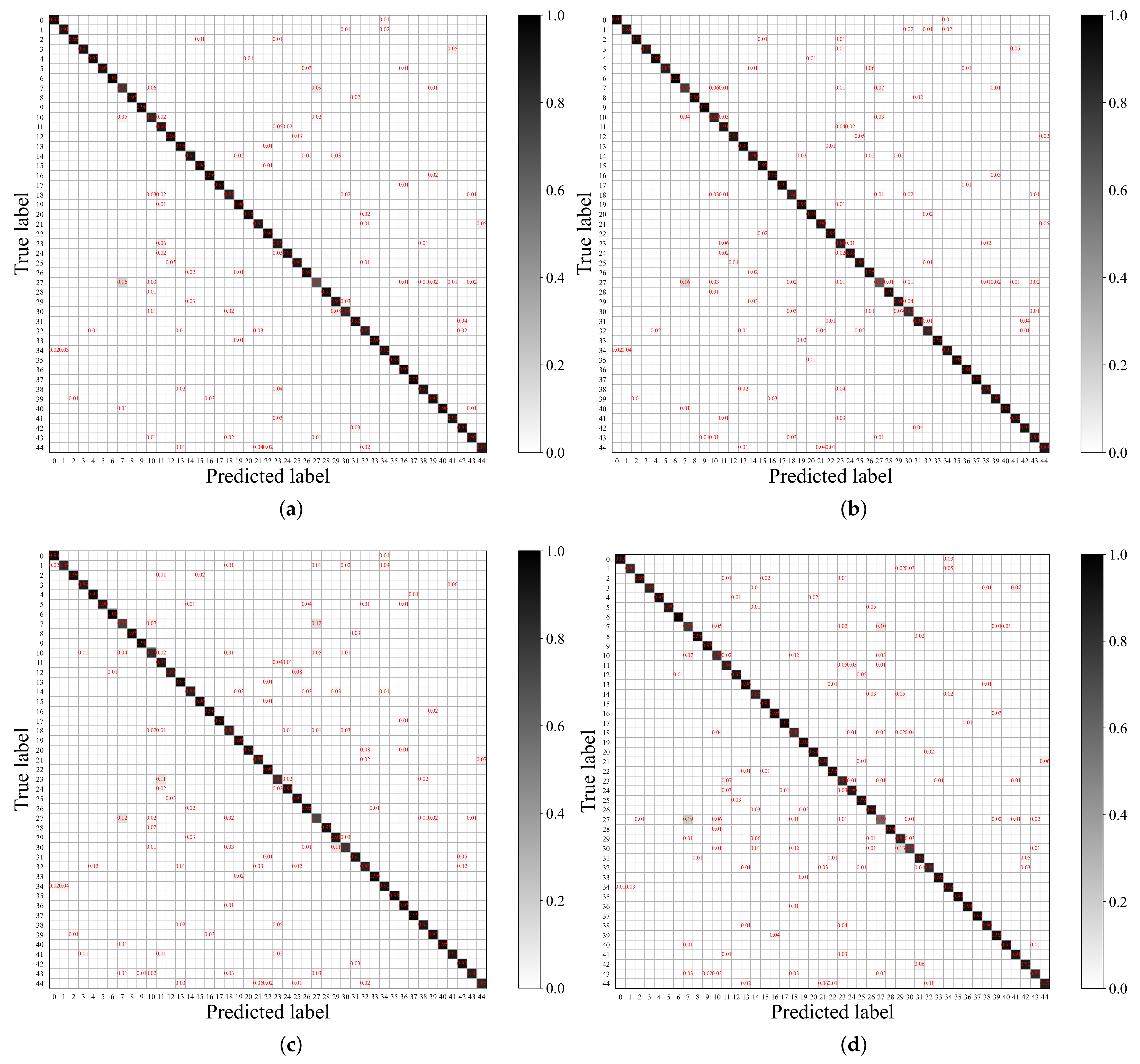
5.2.3. Results on NWPU45

The results of various models counted on NWPU45 are summarized in

Table 3. OA values (%) of different methods on NWPU45 with different noise rates. The best values are marked in bold.

NR	SCE [73]	NCE [74]	RCE [73]	Mixup [75]	NLNL [67]	CMR-NLD [50]	t-RNSL [22]	NTDNE [53]	RS-COCL [54]	Res-PLA (Ours)	MIEN-PLA (Ours)
0.1	84.23	86.56	88.87	85.65	89.37	78.63	88.35	86.25	90.62	92.00	92.35
0.2	78.28	82.15	86.59	82.13	88.62	77.72	86.96	84.77	89.69	91.33	91.70
0.3	69.59	74.75	84.62	74.19	88.20	76.14	85.35	83.27	89.15	90.88	90.97
0.4	61.21	66.52	77.97	67.17	86.67	75.63	82.76	82.00	87.99	89.77	89.88

. Not unexpectedly, the proposed MIEN-PLA achieves first-rate performance in all cases. Compared with the other nine models, the most significant improvements produced by MIEN-PLA are 13.72% (over CMR-NLD, $NR=0.1$), 13.98% (over CMR-NLD, $NR=0.2$), 21.38% (over SCE, $NR=0.3$), and 28.67% (over SCE, $NR=0.4$). In addition, the stability of our models is the best. When $NR$ increases from 0.1 to 0.4, the OA value losses of the compared models are 23.02% (SCE), 20.04% (NCE), 10.90% (RCE), 18.48% (Mixup), 2.70% (NLNL), 3.00% (CMR-NLD), 5.59% (t-RNSL), 4.25% (NTDNE), and 2.63% (RS-COCL). In comparison, PLA and MIEN-PLA’s OA value declines are only 2.23%, which is distinctly smaller than the others. These encouraging investigations prove that the designed MIEN and PLA take the noisy labels into account from various aspects. Hence, more RS scenes with incorrect semantic labels can be recognized, significantly reducing the noisy samples’ impacts.

Figure 11 shows the CMs of our method at different noise rates. For most categories, our MIEN-PLA can achieve adequate results. For example, when $NR=0.4$, the OA values of our method are higher than 90% in 29 out of the 45 classes and are higher than 80% in 38 out of the 45 classes. These promising accomplishments demonstrate the effectiveness of MIEN-PLA. However, we cannot neglect that its behavior is weak in some categories, including “church”, “commercial area”, “freeway”, “medium residential”, “palace”, “railway station”, and “thermal power station”. Especially for “palace”, the OA value is as low as 59%. The main reasons are two-fold. One is the high inter-class similarities (“church”, “commercial area”, “medium residential”, “palace”, and “railway station”), and the other is the sparse and easily-confused contents (“freeway”, and “thermal power station”). Improving our method from these two aspects is one of the goals of our future works.

5.3. Ablation Study

MIEN and PLA are the two critical components of the proposed method in this paper. Thus, we conduct two sets of ablation experiments to study them intensely.

5.3.1. Effectiveness of MIEN

As introduced in Section 4.2, MIEN involves a classification sub-network and a teacher sub-network. Each of them encompasses a ResNet18 and a TAMSFM. To study every component’s contributions, we construct the following nets:

• Net-1: Classification Sub-network without TAMSFM;
• Net-2: Classification Sub-network;
• Net-3: Classification and Teacher Sub-networks.

Net-1 means that we use a single ResNet18 to complete classification. Net-2 indicates that only the classification sub-network is adopted for classifying the RS scenes. Net-3 is actually our MIEN. To train Net-1 and Net-2, the proposed PLA should be modified by removing the outputs of the teacher sub-network. The OA values of different nets counted on three data sets are summarized in

Table 4. OA values (%) of MIEN ablation studies counted on three data sets with different noise rates. The best values are marked in bold.

NR	Nets	Data Set
		UCM	AID	NWPU
0.1	Net-1	98.38	95.06	90.64
	Net-2	98.47	95.22	91.28
	Net-3	98.81	95.72	92.35
0.2	Net-1	97.28	94.38	89.88
	Net-2	97.75	94.71	91.07
	Net-3	98.42	95.27	91.70
0.3	Net-1	96.47	94.12	89.56
	Net-2	96.70	94.38	90.43
	Net-3	97.42	94.81	90.97
0.4	Net-1	95.61	92.98	88.09
	Net-2	95.90	93.27	88.42
	Net-3	96.80	93.44	89.88

. We can see that the performance of the three nets is incremental in all noisy rates. The OA increase of Net-2 compared with Net-1 is 0.29% (UCM21, $NR=0.4$), 0.29% (AID30, $NR=0.4$), and 0.33% (NWPU45, $NR=0.4$). Meanwhile, Net-3 shows an improvement of approximately 0.8% in OA compared to Net-2 across different data sets when $NR=0.4$. These observations illustrate that (i) TAMSFM is beneficial to mining the complex contents within RS scenes and (ii) the dual-branch structure with the specific parameter updating scheme (see Equation (5)) is conducive to reducing the noisy scenes’ influence.

TAMSFM is the key to our MIEN, and the core component of TAMSFM is the CIIT encoder, which is developed based on the ViT encoder by adding CAM into the MSA mechanism (i.e., MISA). To further study the CIIT encoder’s effectiveness, we use other transformer encoders to construct TAMSFM variants. Then, these variants are added to our MIEN to complete the classification. The selected transformer encoders are ViT, efficient multiscale transformer (EMST) encoder [42], Swin transformer (Swin) encoder [76], and Pyramid Vision Transformer (PVT) encoder [77]. We record the variants TAMSFM-V, TAMSFM-E, TAMSFM-S, and TAMSFM-P. For fairness, there is only one encoder in different variants, and their head numbers maintain consistency with the CIIT encoder. The results of MIENs with TAMSFM’s variants are summarized in

Table 5. OA values (%) of MIENs with TAMSFM variants and TAMSFM counted on three data sets ($NR=0.1$). The best values are marked in bold.

	TAMSFM-V	TAMSFM-E	TAMSFM-S	TAMSFM-P	TAMSFM
UCM21	98.42	98.71	98.57	98.47	98.81
AID30	95.25	95.70	95.62	95.44	95.72
NWPU45	92.30	92.33	92.33	92.31	92.35

. For clarity, we only count the scenario of $NR=0.1$.

Through observation, we can find the following conclusions. First, the behavior of TAMSFM-V is the weakest. This is because the VIT encoder is the most primitive and cannot deeply mine the complex contents within RS scenes. Second, TAMSFM-E outperforms other variants. The main reason behind this is that the EMST encoder is designed for the RS classification task, and the multiscale clues extracted are beneficial to understanding RS scenes. Third, the performance of the original TAMSFM is the best. Taking the second-best TAMSFM-E as an example, our TAMSFM exceeds it in OA values by 0.1% (UCM21), 0.02% (AID30), and 0.02% (NWPU45). This shows that our CIIT encoder can fuse information from different views and fully explore long-distance dependencies in RS scenes.

5.3.2. Effectiveness of PLA

PLA has three stages, i.e., DNL, APL, and ESL. To study whether they play a positive role in our method, we perform the following four ablation experiments. First, the original NL and CE losses are adopted to train MIEN, and each is conducted in 40/25 epochs (UCM21) and 50/50 epochs (AID30 and NWPU45) in sequence. Here, the original NL loss means that we do not consider $y_i^t$ when we select the complementary labels (see Equation (6)). We record this experiment as Experiment-1. Experiment-2 adopts the proposed DNL and CE loss to train MIEN. In addition, each stage consists of 50 epochs. This way, the function of DNL can be studied. In Experiment-3, we use DNL and APL to train MIEN to inspect the usefulness of APL. In Experiment-4, DNL, APL, and ESL are leveraged to train our MIEN. This way, the function of ESL can be discovered. Note that the training epochs of different stages in Experiment-3 and Experiment-4 are the same as the settings discussed in Section 5.1.

The results of the four ablation experiments counted on three data sets with different noisy rates are exhibited in

Table 6. OA values (%) of PLA ablation studies counted on three data sets with different noise rates. The best values are marked in bold.

NR	Experiments	DNL	APL	ESL	Data Set
					UCM	AID	NWPU
0.1	Experiment-1	×	×	×	94.28	93.12	89.56
	Experiment-2	✓	×	×	94.76	93.31	89.78
	Experiment-3	✓	✓	×	98.57	95.24	91.64
	Experiment-4	✓	✓	✓	98.81	95.72	92.35
0.2	Experiment-1	×	×	×	89.04	89.62	85.32
	Experiment-2	✓	×	×	89.52	90.14	85.51
	Experiment-3	✓	✓	×	98.10	94.74	91.21
	Experiment-4	✓	✓	✓	98.42	95.27	91.70
0.3	Experiment-1	×	×	×	84.52	84.55	80.57
	Experiment-2	✓	×	×	85.23	84.96	80.92
	Experiment-3	✓	✓	×	97.00	94.62	90.56
	Experiment-4	✓	✓	✓	97.42	94.81	90.97
0.4	Experiment-1	×	×	×	73.57	76.24	73.14
	Experiment-2	✓	×	×	74.04	76.48	73.23
	Experiment-3	✓	✓	×	96.43	93.16	88.52
	Experiment-4	✓	✓	✓	96.80	93.44	89.88

. By observing them, we can see the following points. First, the results of Experiment-2 are better than those of Experiment-1, which implies the usefulness of the DNL stage. This is because introducing the teacher sub-network could help MIEN discover the possible noisy scenes. Hence, the credibility of the complementary labels can be ensured to study the irrelevant relations. Furthermore, the above increase implies that mining the negative relations can enhance the model’s discriminability. Second, distinct performance gaps appear between the results of Experiment-2 and Experiment-3, which illustrates the superiorities of APL. Taking AID30 as an example, the gaps are as high as 1.93% ($NR=0.1$), 4.60% ($NR=0.2$), 9.66% ($NR=0.3$), and 16.68% ($NR=0.4$), respectively. The main reason behind this encouraging observation is that the clean samples selected in the APL stage give our model an excellent classification ability. Third, MIEN performs best in all cases when we add the ESL stage into the training process (Experiment-4). This indicates that ESL plays a positive role in our learning algorithm. In other words, by re-labeling all scenes properly, more useful and correct information within RS scenes can be explored to ensure MIEN’s behavior.

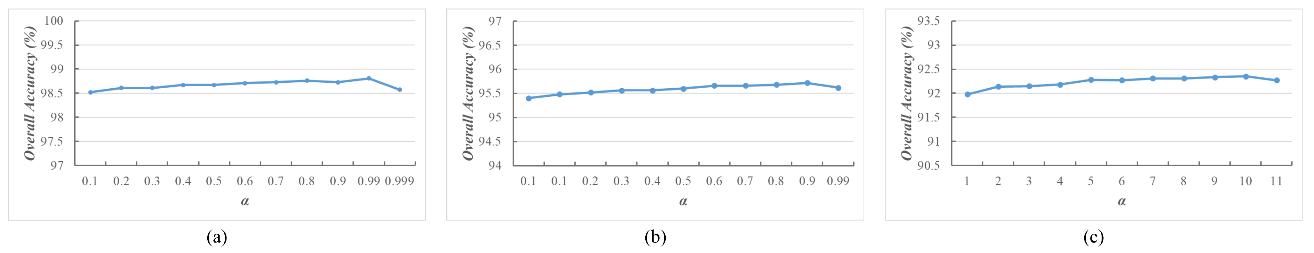
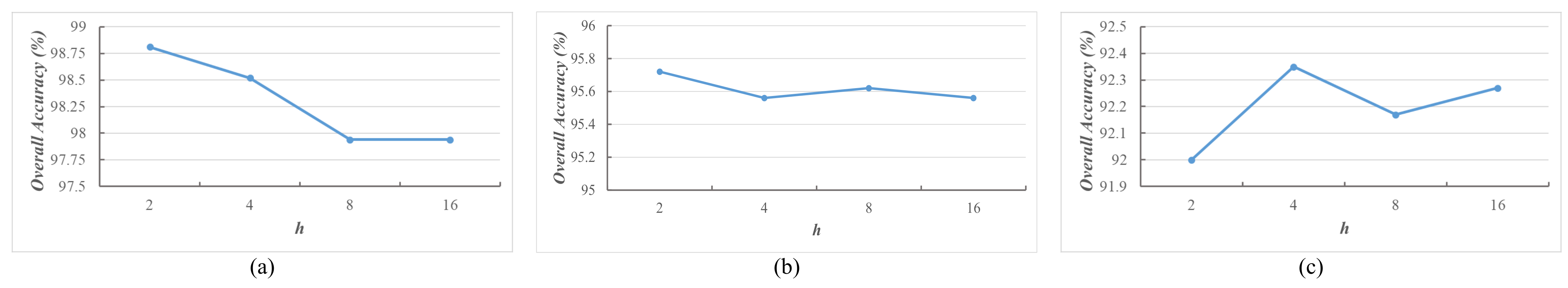
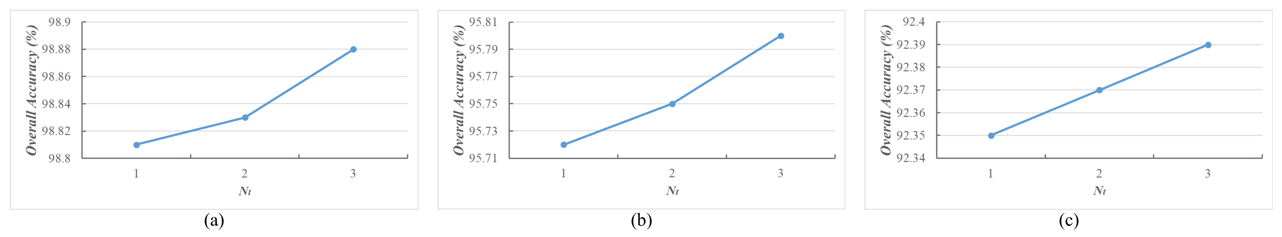
5.4. Sensitivity Analysis

Three free parameters influence our MIEN-PLA, including the smooth transition weight, $\alpha$ (in Equation (5)), the head number of MISA, h (in TAMSFM), and the number of CIIT encoders, $N_t$ (in TAMSFM). In this section, we deeply study their impacts by changing their values individually. First, we fix $h=4$, $N_t=1$, and vary $\alpha$ from 0.1 to 0.9 with an interval of 0.1. In addition, the cases of $\alpha =0.99$ and $\alpha =0.999$ are considered. Next, $\alpha$ and $N_t$ are set to be 0.99 and 1, and h is changed in an range of $\left[2,4,8,16\right]$. Finally, the values of $\alpha$ and h remain, and $N_t$ will be increased from 1 to 3. For clarity, we only analyze the results under $NR=0.1$.

The results of different MIEN-PLAs with diverse $\alpha$ counted on three data sets are shown in Figure 12. From the observation of three figures, we can see that the behavior of MIEN-PLAs becomes stronger when $\alpha$ increases from 0.1 to 0.99. Then, their performance is decreased distinctly when $\alpha$ changes from 0.99 to 0.999. This implies that the teacher sub-network is more dependent on the parameters from the previous iteration rather than the parameters of the classification sub-network in the current iteration. Consequently, the temporal information in the training process can be captured by the teacher sub-network to help MIEN discover the possible noisy RS scenes. Nevertheless, when $\alpha =0.999$, the current and historic knowledge balance is disrupted. Thus, the behavior of MIEN-PLA would be weakened.

The results of various MIEN-PLAs with different h counted on three data sets are shown in Figure 13. For UCM21 and AID30, the behavior of MIEN-PLAs decreases as h increases. For MWPU45, the performance perturbation of MIEN-PLAs is evident. Overall, MIEN-PLA performs optimally on different data sets when h equals 2 or 4. This investigation indicates that MIEN-PLA can learn beneficial messages when the number of projection spaces is small. When projection spaces are enlarged, the excessive fragmentation of information leads to a degradation in MIEN-PLA’s performance.

The OA curves of MIEN-PLAs with varied $N_t$ are exhibited in Figure 14. It is easy to see that MIEN-PLAs become stronger when $N_t$ increases, which implies that the more CIIT encoders there are, the better the performance of MIEN-PLA. However, the parameter volume would be increased dramatically with the increase of $N_t$. In detail, the parameter volume of MIEN-PLAs is 14.60 M, 17.75 M, and 20.90 M when $N_t$ varied from 1 to 3. Considering the trade-off between performance and model size, we suggest $N_t=1$.

5.5. Comparison with Other Classification Models

For RS scene classification with noisy labels, the classification results are decided by the robustness of the learning algorithm and the ability of the feature extractor. In Section 5.2, we demonstrated the effectiveness of our PLA noise tolerance learning algorithm by only using ResNet18 as the backbone of MIEN (i.e., Res-PLA). In this section, we choose several networks designed for RS scenes as the backbones of the classification and teacher sub-networks, including EMTCAL [42], SAGN [26], ACNet [25], and RANet [78], to further study the advancements of our MIEN. The new MIENs are named MIEN-E, MIEN-S, MIEN-A, and MIEN-R, respectively. The above models are trained using PLA, and the backbones’ parameters are set according to the original literature. The OA values of different MIENs under the scenario of $NR=0.1$ are summarized in

Table 7. OA values (%) and GFLOPs of different MIENs trained by PLA counted on three data sets ($NR=0.1$). The best values are marked in bold.

	MIEN-E	MIEN-S	MIEN-A	MIEN-R	MIEN (Ours)
UCM21	98.81	98.75	98.62	98.67	98.81
AID30	95.74	95.64	95.58	95.60	95.72
NWPU45	92.42	92.32	92.12	92.03	92.35
GFLOPs	4.24	4.33	15.35	6.96	2.62

. In addition, Giga floating point operations (GFLOPs) values of different MIENs are provided for reference.

By observing the results, we can see that our MIEN achieves the best OA values on UCM21 and the second-best OA values on AID30 and NWPU45. This proves the superiority of MIEN’s feature extraction capabilities and also reflects that MIEN still has room for improvement when facing large-scale complex RS scene data sets such as AID30 and NWPU45. Although our MIEN is not optimal in OA, its GFLOPs are the best, showing that it is relatively lightweight. In summary, our MIEN is efficient and energetic.

5.6. Time Costs

In this section, we study the efficiency of MIEN-PLA by counting its training and inference times. The time costs of the three RS-oriented methods (i.e., t-RNSL, NTDNE, RS-COCL) are also counted for reference, and their experiment settings are set according to the original literature. We do not adopt CMR-NLD as a comparison because it focuses on filtering noisy samples without useful feature learning. For clarity, we only analyze the results using UCM21 with $NR=0.1$, and the time consumption of different methods is shown in

Table 8. Training time (minute) and inference time (millisecond) of different methods counted on UCM21 at $NR=0.1$.

	t-RNSL [22]	NTDNE [53]	RS-COCL [54]	MIEN-PLA (Ours)
Training. (m)	14.26	14.17	8.33	13.64
Inference. (ms)	11.19	10.42	2.04	2.16

. We can find the following points. First, our MIEN-PLA outperforms t-RNSL and NTDNE in terms of training and inference times, which demonstrates its superiorities. Second, our method spends more time than RS-COCL on the training and inference processes. This is mainly caused by the introduction of TAMSFM. Apart from ResNet18, which is used as the backbone by both RS-COCL and MIEN-PLA, the self-attention mechanism within TAMSFM embedded in ResNet18 significantly increases the training time expenses. Fortunately, the tiny differences between the two methods in the inference stage imply the effectiveness of our MIEN-PLA.

6. Discussion

In this section, we further analyze the differences, advantages, disadvantages, and future directions of our MIEN-PLA in comparison to similar methods.

6.1. Similar Work Comparison

In recent years, noisy RS scene classification has been a hot research topic, and many successful methods have been proposed [50,51,52,53,54,67,73,74,75]. Among them, CMR-NLD [50], RS-COCL [54], and NLNL [67] are similar to our methods as they are also aimed at reducing the impact of noisy labels on the model from different angles and adopt a multi-stage training algorithm. However, the main difference between our MIEN-PLA and these other methods can be summarized as follows. CMR-NLD, RS-COCL, and NLNL focus on filtering out noisy scenes during training, whereas our methods are aimed at discovering the possible noisy data and relabeling them. This way, all samples can be used to train the model, preventing information loss. Meanwhile, compared to two RS-oriented methods (CMR-NLD and RS-COCL), which only use the existing CNNs to generate the visual features, our methods develop a specific network (i.e., MIEN) to explore the multiscale information hidden in RS scenes. This way, the obtained feature representations are more robust.

6.2. Advantages, Weaknesses, and Future Works

The advantages of our MIEN-PLA are two-fold. First, MIEN can deeply explore the complex contents of the RS scenes by analyzing the multiscale clues. Thus, the obtained visual features are strong enough for classification. Second, the simple yet useful PLA can not only discover the possible clean and noisy samples but also use all samples to complete the training, which guarantees the quality of results. Despite the good performance, there is still room for improvement. As shown in Figure 9, Figure 10 and Figure 11, our methods perform weakly in some categories with high intra-class differences and inter-class similarities of RS scenes. In addition, if the scenes contain sparse and easily confused contents (such as “freeway” and “thermal power station”), our model’s performance cannot reach what we expected. Overcoming the above limitations is the goal of our future work.

7. Conclusions

This article proposes a new network (i.e., MIEN) and a learning algorithm (i.e., PLA) for noisy RS scene classification. First, considering the noisy scenarios and characteristics of RS scenes, MIEN is developed to fight against noisy samples and mine the complex contents within RS scenes. By embedding TAMSFM into ResNet18, the local, global, and multiscale information hidden in RS scenes can be fully explored. The possible noisy samples can be recognized intuitively by combining the classification and teacher sub-networks into a dual-branch structure and introducing a simple yet useful parameter-transferring scheme. Second, PLA is designed to train MIEN with noisy samples. PLA consists of three stages, each responsible for a specific task. The DNL stage is aimed at mining the irrelevant relations between RS scenes and complementary labels, which can reduce the training errors caused by noisy samples. The APL stage focuses on finding clean samples. Based on these clean samples and corresponding labels, the performance of MIEN can be improved. The ESL stage focuses on re-labeling all RS scenes and thoroughly training MIEN using the scenes and obtained pseudo-labels. The encouraging results counted on three public data sets demonstrate that our MIEN and PLA can handle RS noisy classification tasks. Compared with many existing methods, the behavior of our network and training algorithm is stronger.

References

1. Zhang, L.; Zhang, L. Artificial Intelligence for Remote Sensing Data Analysis: A review of challenges and opportunities. IEEE Geosci. Remote Sens. Mag. 2022, 10, 270–294. [Google Scholar] [CrossRef]
2. Cheng, G.; Xie, X.; Han, J.; Guo, L.; Xia, G.S. Remote sensing image scene classification meets deep learning: Challenges, methods, benchmarks, and opportunities. IEEE J. Sel. Top. Appl. Earth Obs. Remote Sens. 2020, 13, 3735–3756. [Google Scholar] [CrossRef]
3. Tang, X.; Yang, Y.; Ma, J.; Cheung, Y.M.; Liu, C.; Liu, F.; Zhang, X.; Jiao, L. Meta-hashing for remote sensing image retrieval. IEEE Trans. Geosci. Remote Sens. 2022, 60, 5615419. [Google Scholar] [CrossRef]
4. Xue, J.; Zhao, Y.; Liao, W.; Chan, J.C.W. Nonlocal low-rank regularized tensor decomposition for hyperspectral image denoising. IEEE Trans. Geosci. Remote Sens. 2019, 57, 5174–5189. [Google Scholar] [CrossRef]
5. Tang, X.; Meng, F.; Zhang, X.; Cheung, Y.M.; Ma, J.; Liu, F.; Jiao, L. Hyperspectral image classification based on 3-D octave convolution with spatial–spectral attention network. IEEE Trans. Geosci. Remote Sens. 2020, 59, 2430–2447. [Google Scholar] [CrossRef]
6. Li, Y.; Zhou, Y.; Zhang, Y.; Zhong, L.; Wang, J.; Chen, J. DKDFN: Domain Knowledge-Guided deep collaborative fusion network for multimodal unitemporal remote sensing land cover classification. ISPRS J. Photogramm. Remote Sens. 2022, 186, 170–189. [Google Scholar] [CrossRef]
7. Provost, F.; Michéa, D.; Malet, J.P.; Boissier, E.; Pointal, E.; Stumpf, A.; Pacini, F.; Doin, M.P.; Lacroix, P.; Proy, C.; et al. Terrain deformation measurements from optical satellite imagery: The MPIC-OPT processing services for geohazards monitoring. Remote Sens. Environ. 2022, 274, 112949. [Google Scholar] [CrossRef]
8. De Vroey, M.; De Vendictis, L.; Zavagli, M.; Bontemps, S.; Heymans, D.; Radoux, J.; Koetz, B.; Defourny, P. Mowing detection using Sentinel-1 and Sentinel-2 time series for large scale grassland monitoring. Remote Sens. Environ. 2022, 280, 113145. [Google Scholar] [CrossRef]
9. Zhao, Y.Q.; Yang, J. Hyperspectral image denoising via sparse representation and low-rank constraint. IEEE Trans. Geosci. Remote Sens. 2014, 53, 296–308. [Google Scholar] [CrossRef]
10. Liu, S.; Bai, X.; Zhu, G.; Zhang, Y.; Li, L.; Ren, T.; Lu, J. Remote estimation of leaf nitrogen concentration in winter oilseed rape across growth stages and seasons by correcting for the canopy structural effect. Remote Sens. Environ. 2023, 284, 113348. [Google Scholar] [CrossRef]
11. Gómez-Chova, L.; Tuia, D.; Moser, G.; Camps-Valls, G. Multimodal classification of remote sensing images: A review and future directions. Proc. IEEE 2015, 103, 1560–1584. [Google Scholar] [CrossRef]
12. Chi, M.; Plaza, A.; Benediktsson, J.A.; Sun, Z.; Shen, J.; Zhu, Y. Big data for remote sensing: Challenges and opportunities. Proc. IEEE 2016, 104, 2207–2219. [Google Scholar] [CrossRef]
13. Zhu, X.X.; Tuia, D.; Mou, L.; Xia, G.S.; Zhang, L.; Xu, F.; Fraundorfer, F. Deep learning in remote sensing: A comprehensive review and list of resources. IEEE Geosci. Remote Sens. Mag. 2017, 5, 8–36. [Google Scholar] [CrossRef]
14. Ma, L.; Liu, Y.; Zhang, X.; Ye, Y.; Yin, G.; Johnson, B.A. Deep learning in remote sensing applications: A meta-analysis and review. ISPRS J. Photogramm. Remote Sens. 2019, 152, 166–177. [Google Scholar] [CrossRef]
15. Zhang, B.; Wu, Y.; Zhao, B.; Chanussot, J.; Hong, D.; Yao, J.; Gao, L. Progress and challenges in intelligent remote sensing satellite systems. IEEE J. Sel. Top. Appl. Earth Obs. Remote Sens. 2022, 15, 1814–1822. [Google Scholar] [CrossRef]
16. Han, K.; Wang, Y.; Chen, H.; Chen, X.; Guo, J.; Liu, Z.; Tang, Y.; Xiao, A.; Xu, C.; Xu, Y.; et al. A Survey on Vision Transformer. IEEE Trans. Pattern Anal. Mach. Intell. 2022, 45, 87–110. [Google Scholar] [CrossRef]
17. Khan, S.; Naseer, M.; Hayat, M.; Zamir, S.W.; Khan, F.S.; Shah, M. Transformers in vision: A survey. ACM Comput. Surv. 2022, 54, 1–41. [Google Scholar] [CrossRef]
18. Veit, A.; Alldrin, N.; Chechik, G.; Krasin, I.; Gupta, A.; Belongie, S. Learning from noisy large-scale datasets with minimal supervision. In Proceedings of the IEEE Conference on Computer Vision and Pattern Recognition, Honolulu, HI, USA, 21–26 July 2017; pp. 839–847. [Google Scholar]
19. Han, B.; Tsang, I.W.; Chen, L.; Celina, P.Y.; Fung, S.F. Progressive stochastic learning for noisy labels. IEEE Trans. Neural Netw. Learn. Syst. 2018, 29, 5136–5148. [Google Scholar] [CrossRef]
20. Algan, G.; Ulusoy, I. Image classification with deep learning in the presence of noisy labels: A survey. Knowl. Based Syst. 2021, 215, 106771. [Google Scholar] [CrossRef]
21. Li, Y.; Zhang, Y.; Zhu, Z. Error-Tolerant Deep Learning for Remote Sensing Image Scene Classification. IEEE Trans. Cybern. 2021, 51, 1756–1768. [Google Scholar] [CrossRef] [PubMed]
22. Kang, J.; Fernandez-Beltran, R.; Duan, P.; Kang, X.; Plaza, A.J. Robust normalized softmax loss for deep metric learning-based characterization of remote sensing images with label noise. IEEE Trans. Geosci. Remote Sens. 2020, 59, 8798–8811. [Google Scholar] [CrossRef]
23. Li, J.; Huang, X.; Chang, X. A label-noise robust active learning sample collection method for multi-temporal urban land-cover classification and change analysis. ISPRS J. Photogramm. Remote Sens. 2020, 163, 1–17. [Google Scholar] [CrossRef]
24. He, K.; Zhang, X.; Ren, S.; Sun, J. Deep residual learning for image recognition. In Proceedings of the IEEE Conference on Computer Vision and Pattern Recognition, Las Vegas, NV, USA, 26 June–1 July 2016; pp. 770–778. [Google Scholar]
25. Tang, X.; Ma, Q.; Zhang, X.; Liu, F.; Ma, J.; Jiao, L. Attention consistent network for remote sensing scene classification. IEEE J. Sel. Top. Appl. Earth Obs. Remote Sens. 2021, 14, 2030–2045. [Google Scholar] [CrossRef]
26. Yang, Y.; Tang, X.; Cheung, Y.M.; Zhang, X.; Jiao, L. SAGN: Semantic-Aware Graph Network for Remote Sensing Scene Classification. IEEE Trans. Image Process. 2023, 32, 1011–1025. [Google Scholar] [CrossRef]
27. Wang, X.; Wang, S.; Ning, C.; Zhou, H. Enhanced feature pyramid network with deep semantic embedding for remote sensing scene classification. IEEE Trans. Geosci. Remote Sens. 2021, 59, 7918–7932. [Google Scholar] [CrossRef]
28. Liu, C.; Ma, J.; Tang, X.; Liu, F.; Zhang, X.; Jiao, L. Deep hash learning for remote sensing image retrieval. IEEE Trans. Geosci. Remote Sens. 2020, 59, 3420–3443. [Google Scholar] [CrossRef]
29. Chen, J.; Huang, H.; Peng, J.; Zhu, J.; Chen, L.; Tao, C.; Li, H. Contextual information-preserved architecture learning for remote-sensing scene classification. IEEE Trans. Geosci. Remote Sens. 2021, 60, 5602614. [Google Scholar] [CrossRef]
30. Bi, Q.; Qin, K.; Zhang, H.; Xia, G.S. Local semantic enhanced convnet for aerial scene recognition. IEEE Trans. Image Process. 2022, 30, 6498–6511. [Google Scholar] [CrossRef]
31. Guo, N.; Jiang, M.; Gao, L.; Li, K.; Zheng, F.; Chen, X.; Wang, M. HFCC-Net: A Dual-Branch Hybrid Framework of CNN and CapsNet for Land-Use Scene Classification. Remote Sens. 2023, 15, 5044. [Google Scholar] [CrossRef]
32. Tang, X.; Lin, W.; Ma, J.; Zhang, X.; Liu, F.; Jiao, L. Class-Level Prototype Guided Multiscale Feature Learning for Remote Sensing Scene Classification With Limited Labels. IEEE Trans. Geosci. Remote Sens. 2022, 60, 5622315. [Google Scholar] [CrossRef]
33. Li, X.; Shi, D.; Diao, X.; Xu, H. SCL-MLNet: Boosting Few-Shot Remote Sensing Scene Classification via Self-Supervised Contrastive Learning. IEEE Trans. Geosci. Remote Sens. 2022, 60, 5801112. [Google Scholar] [CrossRef]
34. Peng, C.; Li, Y.; Jiao, L.; Shang, R. Efficient convolutional neural architecture search for remote sensing image scene classification. IEEE Trans. Geosci. Remote Sens. 2020, 59, 6092–6105. [Google Scholar] [CrossRef]
35. Vaswani, A.; Shazeer, N.; Parmar, N.; Uszkoreit, J.; Jones, L.; Gomez, A.N.; Kaiser, L.; Polosukhin, I. Attention is all you need. In Proceedings of the Advances in Neural Information Processing Systems, Long Beach, CA, USA, 4–9 December 2017; Volume 30. [Google Scholar]
36. Dosovitskiy, A.; Beyer, L.; Kolesnikov, A.; Weissenborn, D.; Zhai, X.; Unterthiner, T.; Dehghani, M.; Minderer, M.; Heigold, G.; Gelly, S.; et al. An image is worth 16×16 words: Transformers for image recognition at scale. arXiv 2020, arXiv:2010.11929. [Google Scholar]
37. Li, Y.; Yao, T.; Pan, Y.; Mei, T. Contextual transformer networks for visual recognition. IEEE Trans. Pattern Anal. Mach. Intell. 2022, 45, 1489–1500. [Google Scholar] [CrossRef] [PubMed]
38. Lin, H.; Cheng, X.; Wu, X.; Shen, D. Cat: Cross attention in vision transformer. In Proceedings of the 2022 IEEE International Conference on Multimedia and Expo, Taipei, China, 18–22 July 2022; pp. 1–6. [Google Scholar]
39. Huang, X.; Bi, N.; Tan, J. Visual Transformer-Based Models: A Survey. In Proceedings of the International Conference on Pattern Recognition and Artificial Intelligence, Xiamen, China, 23–25 September 2022; pp. 295–305. [Google Scholar]
40. Ma, J.; Li, M.; Tang, X.; Zhang, X.; Liu, F.; Jiao, L. Homo–Heterogenous Transformer Learning Framework for RS Scene Classification. IEEE J. Sel. Top. Appl. Earth Obs. Remote Sens. 2022, 15, 2223–2239. [Google Scholar] [CrossRef]
41. Lv, P.; Wu, W.; Zhong, Y.; Du, F.; Zhang, L. SCViT: A Spatial-Channel Feature Preserving Vision Transformer for Remote Sensing Image Scene Classification. IEEE Trans. Geosci. Remote Sens. 2022, 60, 4409512. [Google Scholar] [CrossRef]
42. Tang, X.; Li, M.; Ma, J.; Zhang, X.; Liu, F.; Jiao, L. EMTCAL: Efficient Multiscale Transformer and Cross-Level Attention Learning for Remote Sensing Scene Classification. IEEE Trans. Geosci. Remote Sens. 2022, 60, 5626915. [Google Scholar] [CrossRef]
43. Xu, K.; Deng, P.; Huang, H. Vision transformer: An excellent teacher for guiding small networks in remote sensing image scene classification. IEEE Trans. Geosci. Remote Sens. 2022, 60, 5618715. [Google Scholar] [CrossRef]
44. Li, Y.; Zhu, Z.; Yu, J.G.; Zhang, Y. Learning deep cross-modal embedding networks for zero-shot remote sensing image scene classification. IEEE Trans. Geosci. Remote Sens. 2021, 59, 10590–10603. [Google Scholar] [CrossRef]
45. Zhou, L.; Liu, Y.; Zhang, P.; Bai, X.; Gu, L.; Zhou, J.; Yao, Y.; Harada, T.; Zheng, J.; Hancock, E. Information bottleneck and selective noise supervision for zero-shot learning. Mach. Learn. 2023, 112, 2239–2261. [Google Scholar] [CrossRef]
46. Li, Z.; Zhang, D.; Wang, Y.; Lin, D.; Zhang, J. Generative adversarial networks for zero-shot remote sensing scene classification. Appl. Sci. 2022, 12, 3760. [Google Scholar] [CrossRef]
47. Pradhan, B.; Al-Najjar, H.A.; Sameen, M.I.; Tsang, I.; Alamri, A.M. Unseen land cover classification from high-resolution orthophotos using integration of zero-shot learning and convolutional neural networks. Remote Sens. 2020, 12, 1676. [Google Scholar] [CrossRef]
48. Zhang, Y.; Sun, J.; Shi, H.; Ge, Z.; Yu, Q.; Cao, G.; Li, X. Agreement and Disagreement-Based Co-Learning with Dual Network for Hyperspectral Image Classification with Noisy Labels. Remote Sens. 2023, 15, 2543. [Google Scholar] [CrossRef]
49. Zheng, G.; Awadallah, A.H.; Dumais, S. Meta label correction for noisy label learning. In Proceedings of the AAAI Conference on Artificial Intelligence, Virtual, 2–9 February 2021; Volume 35, pp. 11053–11061. [Google Scholar]
50. Tu, B.; Kuang, W.; He, W.; Zhang, G.; Peng, Y. Robust learning of mislabeled training samples for remote sensing image scene classification. IEEE J. Sel. Top. Appl. Earth Obs. Remote Sens. 2020, 13, 5623–5639. [Google Scholar] [CrossRef]
51. Zhang, R.; Chen, Z.; Zhang, S.; Song, F.; Zhang, G.; Zhou, Q.; Lei, T. Remote sensing image scene classification with noisy label distillation. Remote Sens. 2020, 12, 2376. [Google Scholar] [CrossRef]
52. Li, Y.; Zhang, Y.; Zhu, Z. Learning deep networks under noisy labels for remote sensing image scene classification. In Proceedings of the IGARSS 2019—2019 IEEE International Geoscience and Remote Sensing Symposium, Yokohama, Japan, 28 July–2 August 2019; pp. 3025–3028. [Google Scholar]
53. Kang, J.; Fernandez-Beltran, R.; Kang, X.; Ni, J.; Plaza, A. Noise-tolerant deep neighborhood embedding for remotely sensed images with label noise. IEEE J. Sel. Top. Appl. Earth Obs. Remote Sens. 2021, 14, 2551–2562. [Google Scholar] [CrossRef]
54. Li, Q.; Chen, Y.; Ghamisi, P. Complementary learning-based scene classification of remote sensing images with noisy labels. IEEE Geosci. Remote Sens. Lett. 2021, 19, 8021105. [Google Scholar] [CrossRef]
55. Yang, Y.; Newsam, S. Bag-of-visual-words and spatial extensions for land-use classification. In Proceedings of the 18th SIGSPATIAL International Conference on Advances in Geographic Information Systems, San Jose, CA, USA, 2–5 November 2010; pp. 270–279. [Google Scholar]
56. Xia, G.S.; Hu, J.; Hu, F.; Shi, B.; Bai, X.; Zhong, Y.; Zhang, L.; Lu, X. AID: A benchmark data set for performance evaluation of aerial scene classification. IEEE Trans. Geosci. Remote Sens. 2017, 55, 3965–3981. [Google Scholar] [CrossRef]
57. Cheng, G.; Han, J.; Lu, X. Remote sensing image scene classification: Benchmark and state of the art. Proc. IEEE 2017, 105, 1865–1883. [Google Scholar] [CrossRef]
58. Miao, W.; Geng, J.; Jiang, W. Multigranularity Decoupling Network With Pseudolabel Selection for Remote Sensing Image Scene Classification. IEEE Trans. Geosci. Remote Sens. 2023, 61, 5603813. [Google Scholar] [CrossRef]
59. Xu, Q.; Shi, Y.; Yuan, X.; Zhu, X.X. Universal Domain Adaptation for Remote Sensing Image Scene Classification. IEEE Trans. Geosci. Remote Sens. 2023, 61, 4700515. [Google Scholar] [CrossRef]
60. Yang, Y.; Tang, X.; Zhang, X.; Ma, J.; Liu, F.; Jia, X.; Jiao, L. Semi-Supervised Multiscale Dynamic Graph Convolution Network for Hyperspectral Image Classification. IEEE Trans. Neural Netw. Learn. Syst. 2022. early access. [Google Scholar] [CrossRef]
61. Lu, X.; Sun, H.; Zheng, X. A feature aggregation convolutional neural network for remote sensing scene classification. IEEE Trans. Geosci. Remote Sens. 2019, 57, 7894–7906. [Google Scholar] [CrossRef]
62. Wang, X.; Duan, L.; Ning, C. Global context-based multilevel feature fusion networks for multilabel remote sensing image scene classification. IEEE J. Sel. Top. Appl. Earth Obs. Remote Sens. 2021, 14, 11179–11196. [Google Scholar] [CrossRef]
63. Li, J.; Socher, R.; Hoi, S.C. Dividemix: Learning with noisy labels as semi-supervised learning. arXiv 2020, arXiv:2002.07394. [Google Scholar]
64. Tan, C.; Xia, J.; Wu, L.; Li, S.Z. Co-learning: Learning from noisy labels with self-supervision. In Proceedings of the 29th ACM International Conference on Multimedia, Virtual, China, 20–24 October 2021; pp. 1405–1413. [Google Scholar]
65. Li, S.; Xia, X.; Ge, S.; Liu, T. Selective-supervised contrastive learning with noisy labels. In Proceedings of the IEEE/CVF Conference on Computer Vision and Pattern Recognition, New Orleans, LA, USA, 18–24 June 2022; pp. 316–325. [Google Scholar]
66. Tarvainen, A.; Valpola, H. Mean teachers are better role models: Weight-averaged consistency targets improve semi-supervised deep learning results. In Proceedings of the Advances in Neural Information Processing Systems, Long Beach, CA, USA, 4–9 December 2017; Volume 30. [Google Scholar]
67. Kim, Y.; Yim, J.; Yun, J.; Kim, J. Nlnl: Negative learning for noisy labels. In Proceedings of the IEEE/CVF International Conference on Computer Vision, Seoul, Korea, 27 October–2 November 2019; pp. 101–110. [Google Scholar]
68. Song, H.; Kim, M.; Park, D.; Shin, Y.; Lee, J.G. Learning from noisy labels with deep neural networks: A survey. IEEE Trans. Neural Netw. Learn. Syst. 2022, 34, 8135–8153. [Google Scholar] [CrossRef] [PubMed]
69. Szegedy, C.; Vanhoucke, V.; Ioffe, S.; Shlens, J.; Wojna, Z. Rethinking the inception architecture for computer vision. In Proceedings of the IEEE Conference on Computer Vision and Pattern Recognition, Las Vegas, NV, USA, 26 June–1 July 2016; pp. 2818–2826. [Google Scholar]
70. Paszke, A.; Gross, S.; Massa, F.; Lerer, A.; Bradbury, J.; Chanan, G.; Killeen, T.; Lin, Z.; Gimelshein, N.; Antiga, L.; et al. Pytorch: An imperative style, high-performance deep learning library. In Proceedings of the Advances in Neural Information Processing Systems, Vancouver, BC, Canada, 8–14 December 2019; Volume 32. [Google Scholar]
71. Krizhevsky, A.; Sutskever, I.; Hinton, G.E. Imagenet classification with deep convolutional neural networks. Commun. ACM 2017, 60, 84–90. [Google Scholar] [CrossRef]
72. Han, B.; Yao, Q.; Yu, X.; Niu, G.; Xu, M.; Hu, W.; Tsang, I.; Sugiyama, M. Co-teaching: Robust training of deep neural networks with extremely noisy labels. In Proceedings of the Advances in Neural Information Processing Systems, Montreal, QC, Canada, 3–8 December 2018 2018; Volume 31. [Google Scholar]
73. Wang, Y.; Ma, X.; Chen, Z.; Luo, Y.; Yi, J.; Bailey, J. Symmetric cross entropy for robust learning with noisy labels. In Proceedings of the IEEE/CVF International Conference on Computer Vision, Seoul, Republic of Korea, 27 October–2 November 2019; pp. 322–330. [Google Scholar]
74. Ma, X.; Huang, H.; Wang, Y.; Romano, S.; Erfani, S.; Bailey, J. Normalized loss functions for deep learning with noisy labels. In Proceedings of the International Conference on Machine Learning, Virtual, 13–18 July 2020; pp. 6543–6553. [Google Scholar]
75. Zhang, H.; Cisse, M.; Dauphin, Y.N.; Lopez-Paz, D. mixup: Beyond empirical risk minimization. arXiv 2017, arXiv:1710.09412. [Google Scholar]
76. Liu, Z.; Lin, Y.; Cao, Y.; Hu, H.; Wei, Y.; Zhang, Z.; Lin, S.; Guo, B. Swin transformer: Hierarchical vision transformer using shifted windows. In Proceedings of the IEEE/CVF International Conference on Computer Vision, Nashville, TN, USA, 20–25 June 2021; pp. 10012–10022. [Google Scholar]
77. Wang, W.; Xie, E.; Li, X.; Fan, D.P.; Song, K.; Liang, D.; Lu, T.; Luo, P.; Shao, L. Pyramid vision transformer: A versatile backbone for dense prediction without convolutions. In Proceedings of the IEEE/CVF International Conference on Computer Vision, Nashville, TN, USA, 20–25 June 2021; pp. 568–578. [Google Scholar]
78. Wang, X.; Duan, L.; Ning, C.; Zhou, H. Relation-attention networks for remote sensing scene classification. IEEE J. Sel. Top. Appl. Earth Obs. Remote Sens. 2021, 15, 422–439. [Google Scholar] [CrossRef]
Figure 1. Examples and their serial numbers and semantics of the UCM21 data set.
Remotesensing 15 05706 g001
Figure 2. Examples and their serial numbers and semantics of the AID30 data set.
Remotesensing 15 05706 g002
Figure 3. Examples and their serial numbers and semantics of the NWPU45 data set.
Remotesensing 15 05706 g003
Figure 4. Framework of the proposed method, which consists of a multiscale information exploration network (MIEN) and a progressive learning algorithm (PLA).
Remotesensing 15 05706 g004
Figure 5. Framework of the classification sub-network, which mainly contains a ResNet18 and a transformer-assistive multiscale fusion module.
Remotesensing 15 05706 g005
Figure 6. Structure of a cross-head information interaction transformer (CIIT) encoder, which encloses a multi-head interaction self-attention (MISA) block and a multi-layer perception block in a residual way.
Remotesensing 15 05706 g006
Figure 7. Framework of the multi-head self-attention (MSA) and multi-head interaction self-attention (MISA) mechanisms. (a) MSA. (b) MISA.
Remotesensing 15 05706 g007
Figure 8. Structure of the cross-head associating module (CAM), taking M 1 interacting with other attention maps as an example.
Remotesensing 15 05706 g008
Figure 9. Confusion matrices of the proposed MIEN-PLA counted on UCM21 at different noise rates. (a) N R = 0.1 . (b) N R = 0.2 . (c) N R = 0.3 . (d) N R = 0.4 . The semantics corresponding to the serial numbers can be found in Figure 1.
Remotesensing 15 05706 g009
Figure 10. Confusion matrices of the proposed MIEN-PLA counted on AID30 at different noise rates. (a) N R = 0.1 . (b) N R = 0.2 . (c) N R = 0.3 . (d) N R = 0.4 . The semantics corresponding to the serial numbers can be found in Figure 2.
Remotesensing 15 05706 g010
Figure 11. Confusion matrices of the proposed MIEN-PLA counted on NWPU45 at different noise rates. (a) N R = 0.1 . (b) N R = 0.2 . (c) N R = 0.3 . (d) N R = 0.4 . The semantics corresponding to the serial numbers can be found in Figure 3.
Remotesensing 15 05706 g011
Figure 12. OA values of different MIEN-PLAs with different α counted on three data sets ( N R = 0.1 ). (a) UCM21. (b) AID30. (c) NWPU45.
Remotesensing 15 05706 g012
Figure 13. OA values of different MIEN-PLAs with different h counted on three data sets ( N R = 0.1 ). (a) UCM21. (b) AID30. (c) NWPU45.
Remotesensing 15 05706 g013
Figure 14. OA values of different MIEN-PLAs with different N t counted on three data sets ( N R = 0.1 ). (a) UCM21. (b) AID30. (c) NWPU45.
Remotesensing 15 05706 g014