
Beyond Pixel-Wise Unmixing: Spatial–Spectral Attention Fully Convolutional Networks for Abundance Estimation


Abstract
:1. Introduction
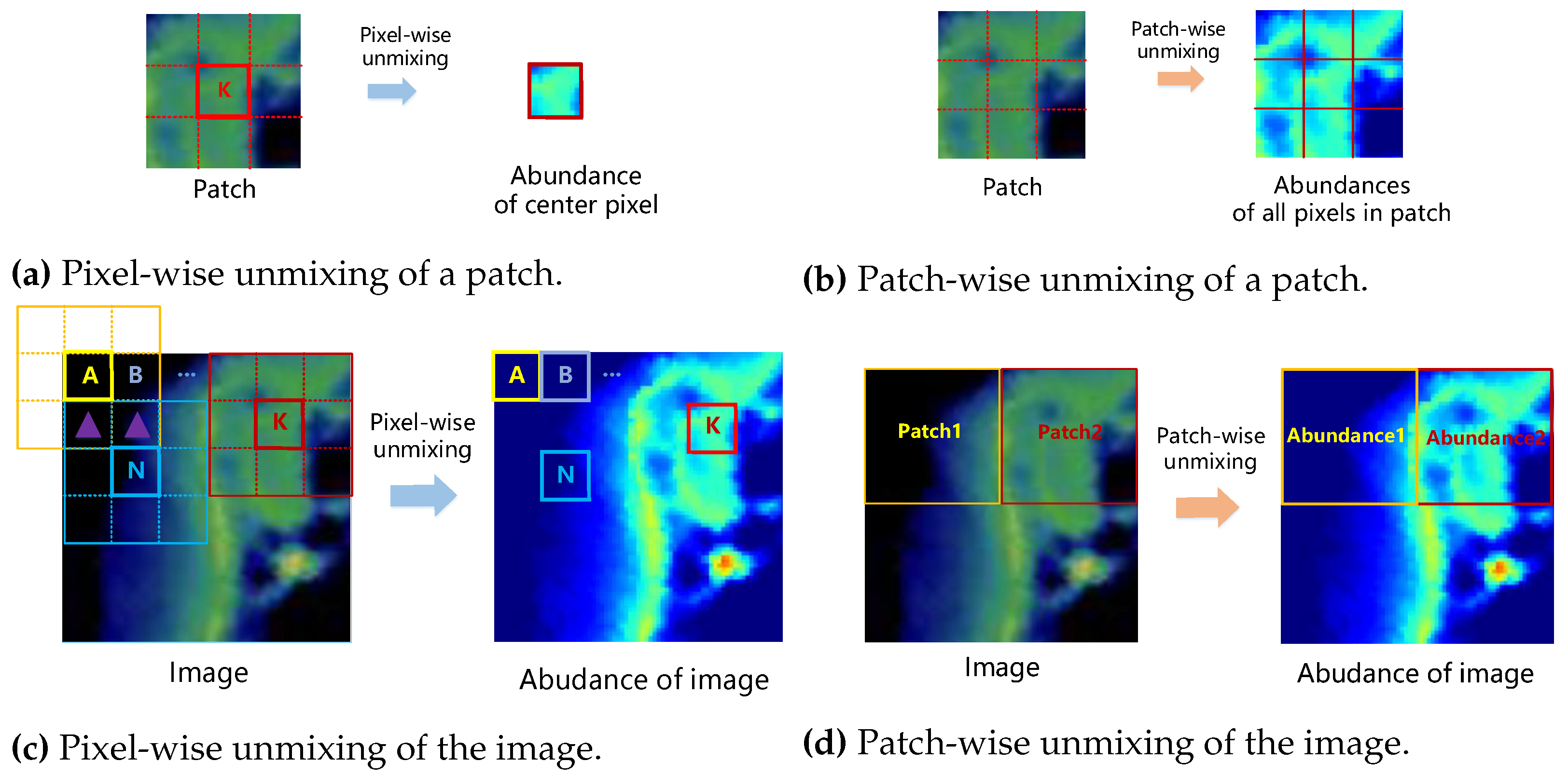
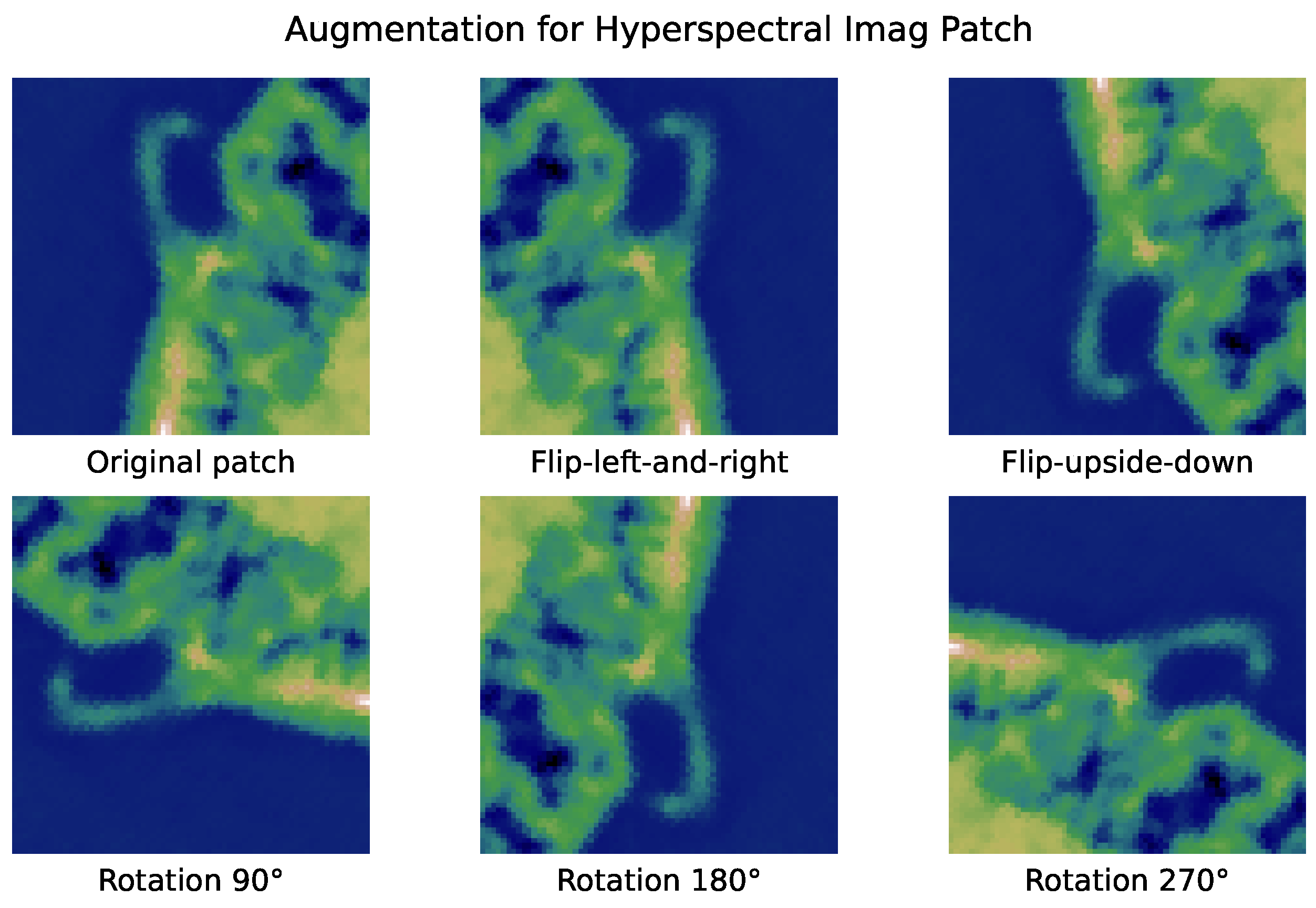
- Beyond the conventional pixel-wise framework commonly employed in CNN unmixing, we introduce a patch-wise unmixing method, facilitating the mapping of image patches to abundance patches. This approach allows for nonoverlapping splitting, eliminating the need to recompute overlapping pixels and mitigating information leakage between the training and test sets, ensuring a fair evaluation.
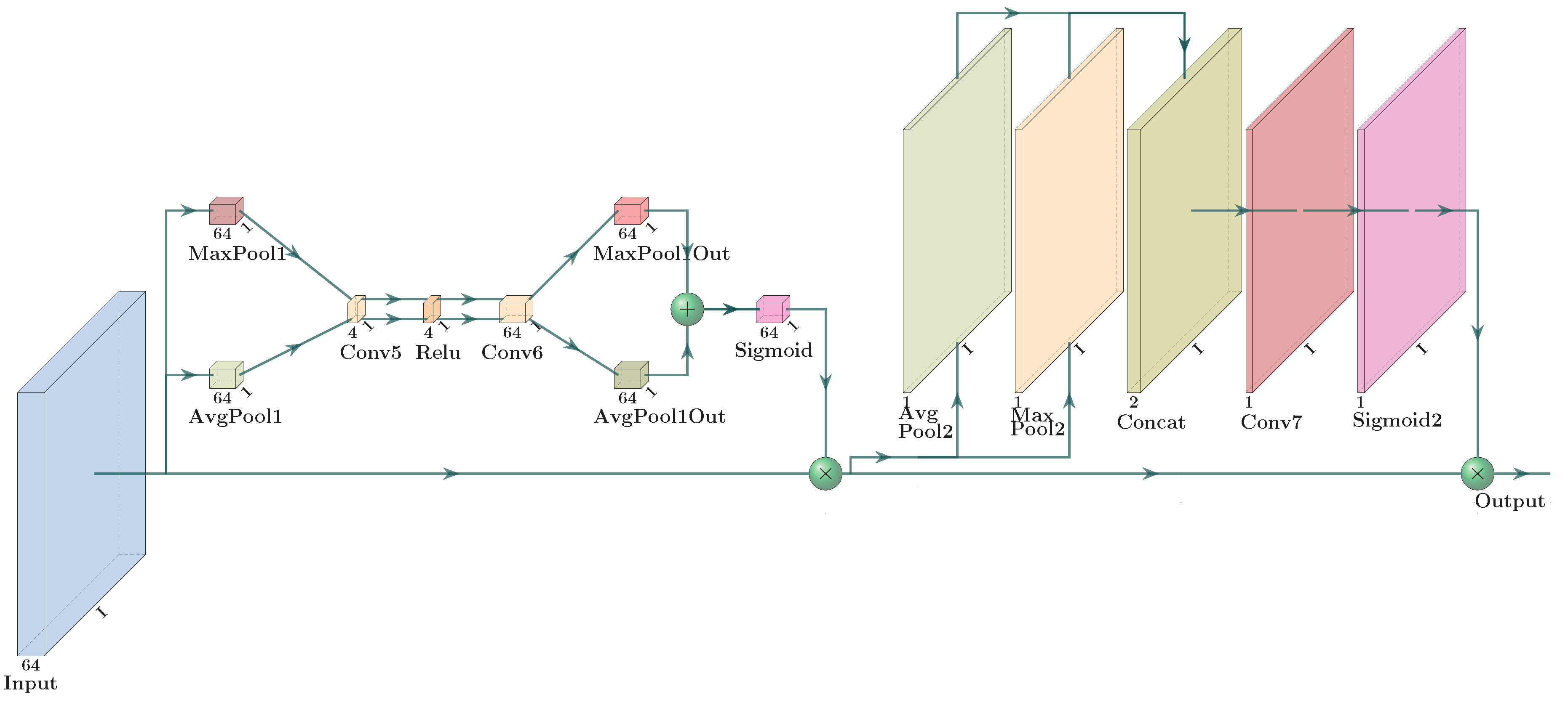
- A novel convolutional-transposed convolutional structure is meticulously designed. The inclusion of a band reduction convolutional layer effectively reduces the dimensionality of bands, facilitating the extraction of spectral features crucial for accurate unmixing. The fusion of spatial and spectral attention networks enables the model to selectively emphasize informative spatial areas and spectral features, thereby enhancing the performance of abundance estimation. Additionally, a weighted regression loss, combining and , is proposed to guide the optimization process in hyperspectral unmixing.
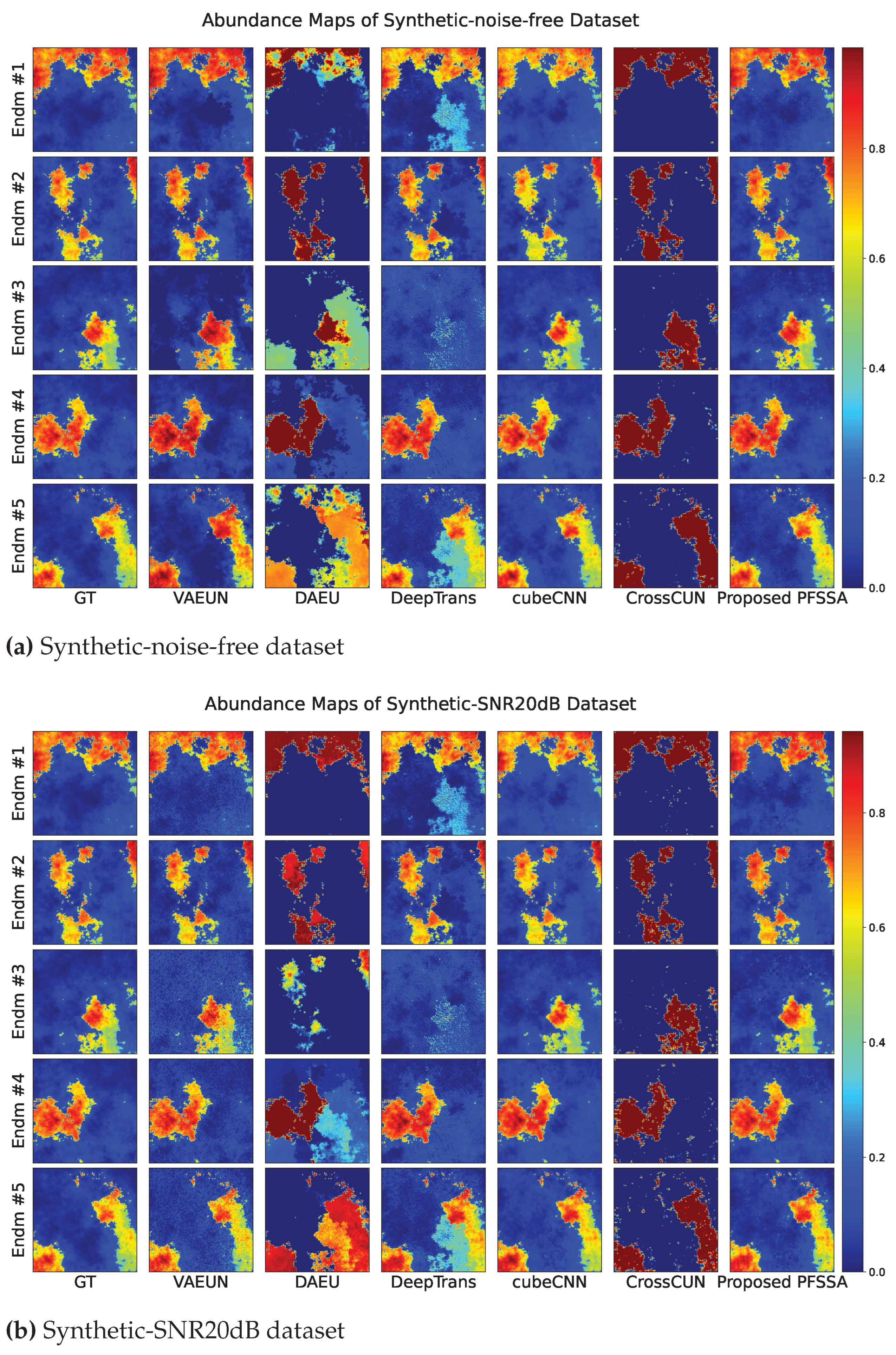
- The comparative quantitative experimental results and visual assessments of abundance on two synthetic datasets and three real hyperspectral images validate the superiority of the designed network. Notably, the proposed algorithm significantly outperforms other baselines on synthetic data and Samson data, achieving at least a 4.5-fold improvement in over other baselines on the Urban image.
2. Related Work
3. Methodology
3.1. Preliminary
3.2. The Patch-Wise Unmixing Framework
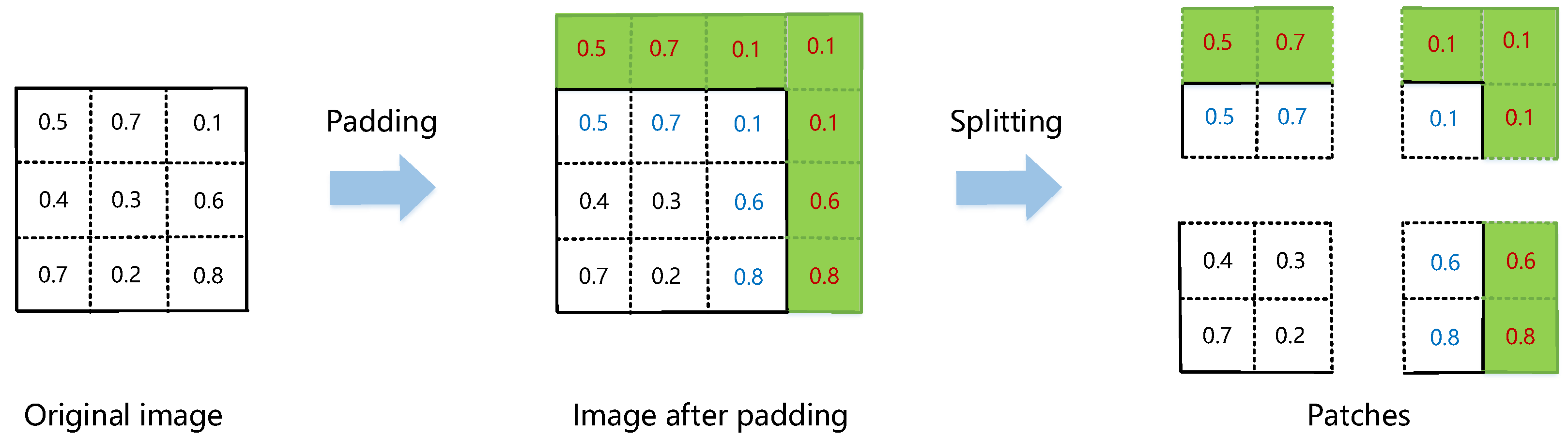
3.2.1. Image Padding and Splitting
3.2.2. Patch Unmixing
3.2.3. Abundance Joining and Cropping
3.3. Weighted Loss
4. Experiments
4.1. Experimental setting
4.1.1. Data Description
- (1)
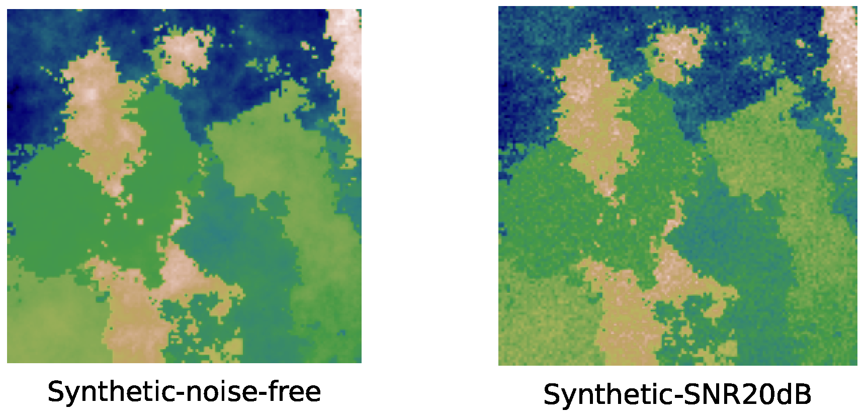
- Synthetic data
- (2)
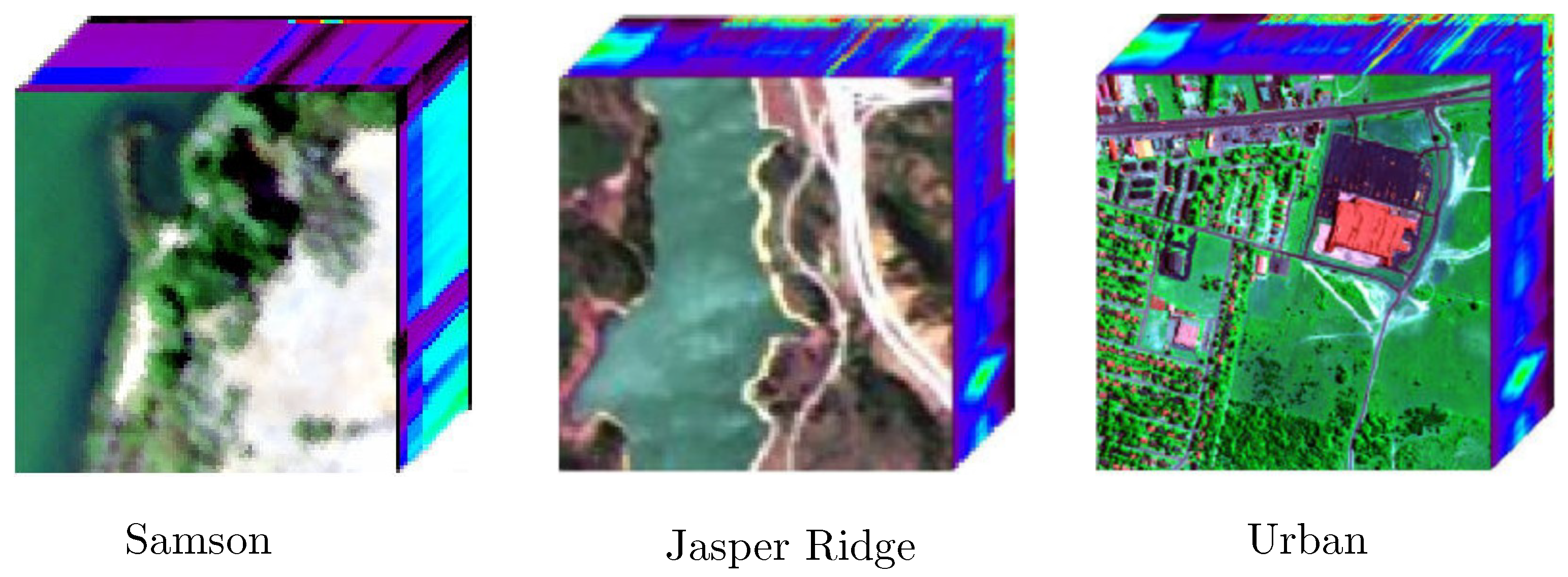
- Real Data
4.1.2. Baselines
4.1.3. Implementation Details
4.2. Results Analysis and Visual Evaluation
4.2.1. Results of Synthetic Data
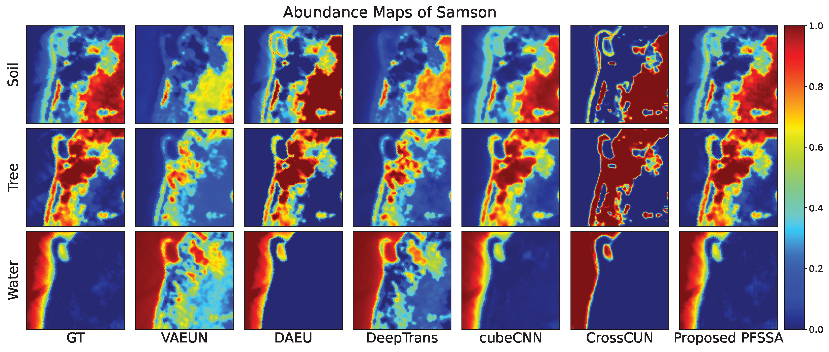
4.2.2. Results of Samson Data
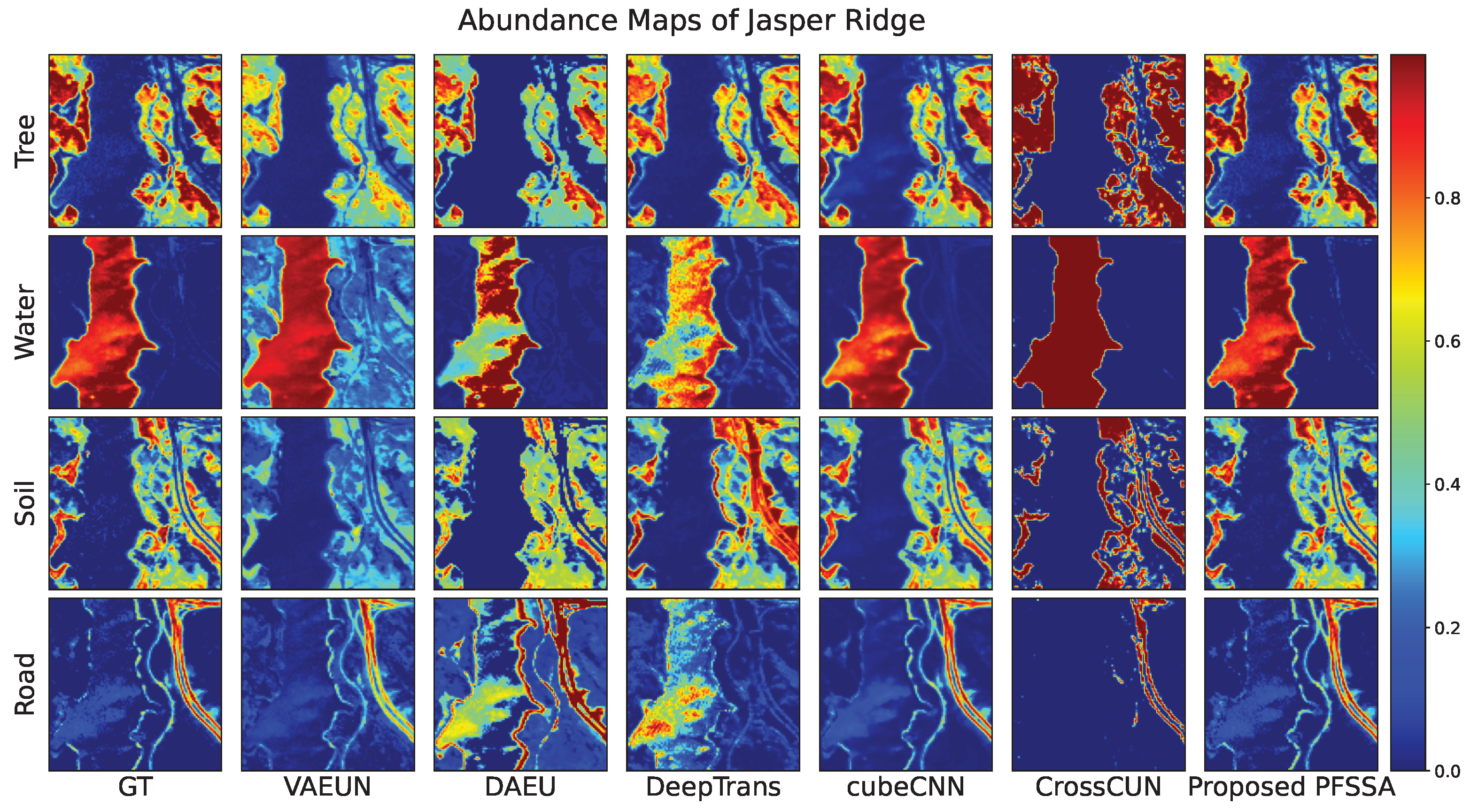
4.2.3. Results of Jasper Ridge Data
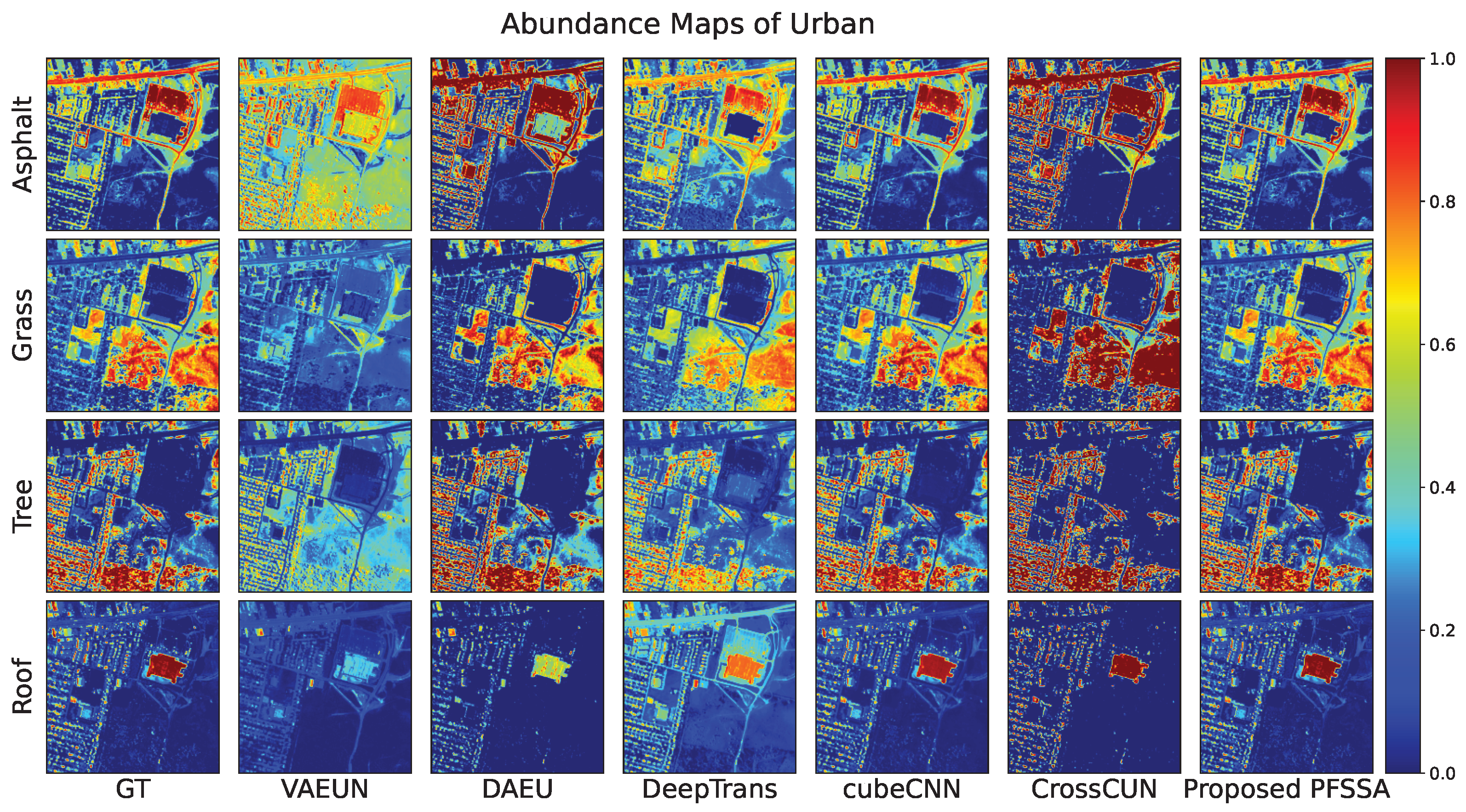
4.2.4. Results of Urban Data
4.3. Ablation Study and Parameter Analysis
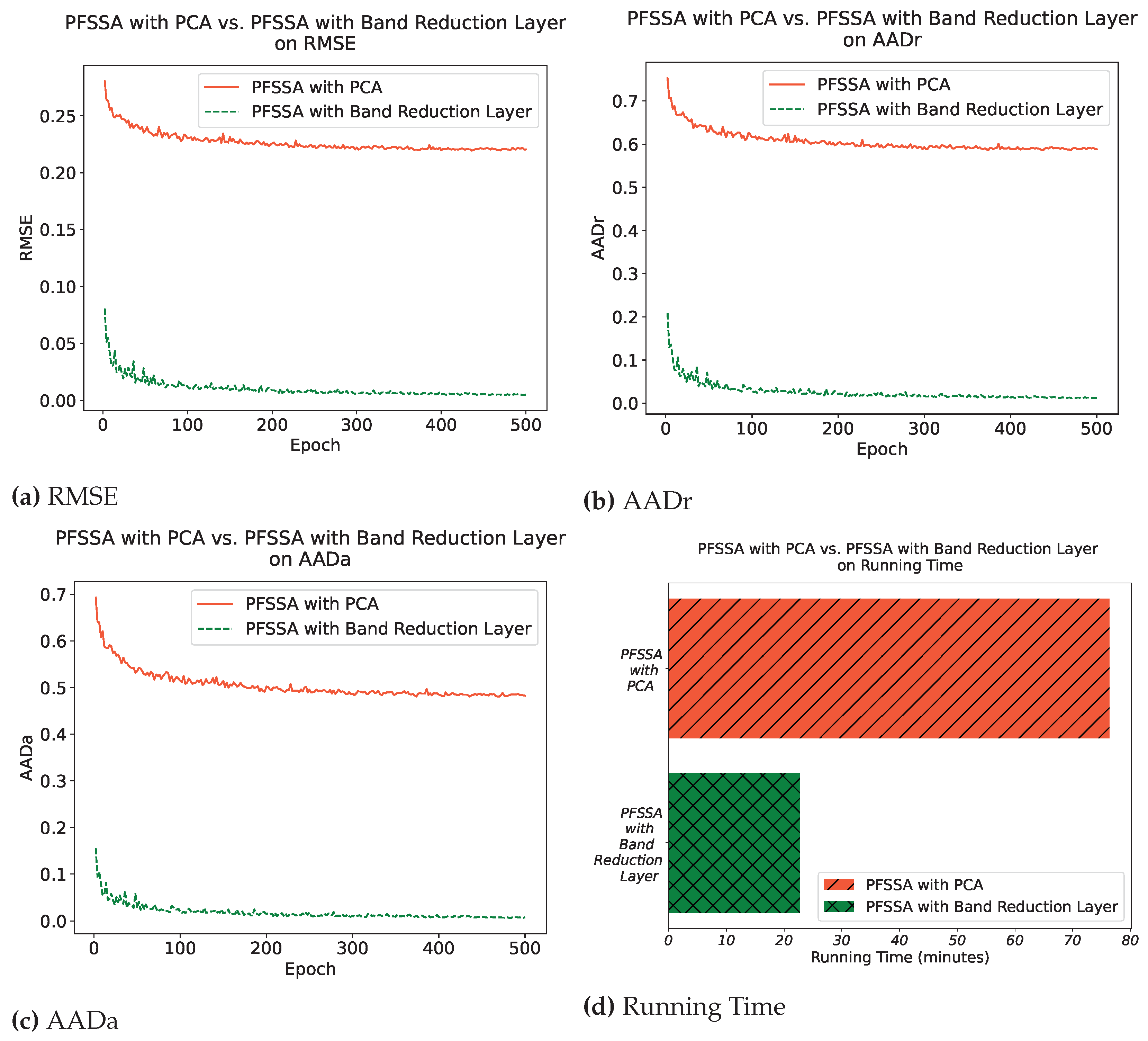
4.3.1. Comparing Band Reduction Layer with PCA
4.3.2. Ablation Study on Spatial–Spectral Attention
4.3.3. Padding modes
4.3.4. Training Set Ratio
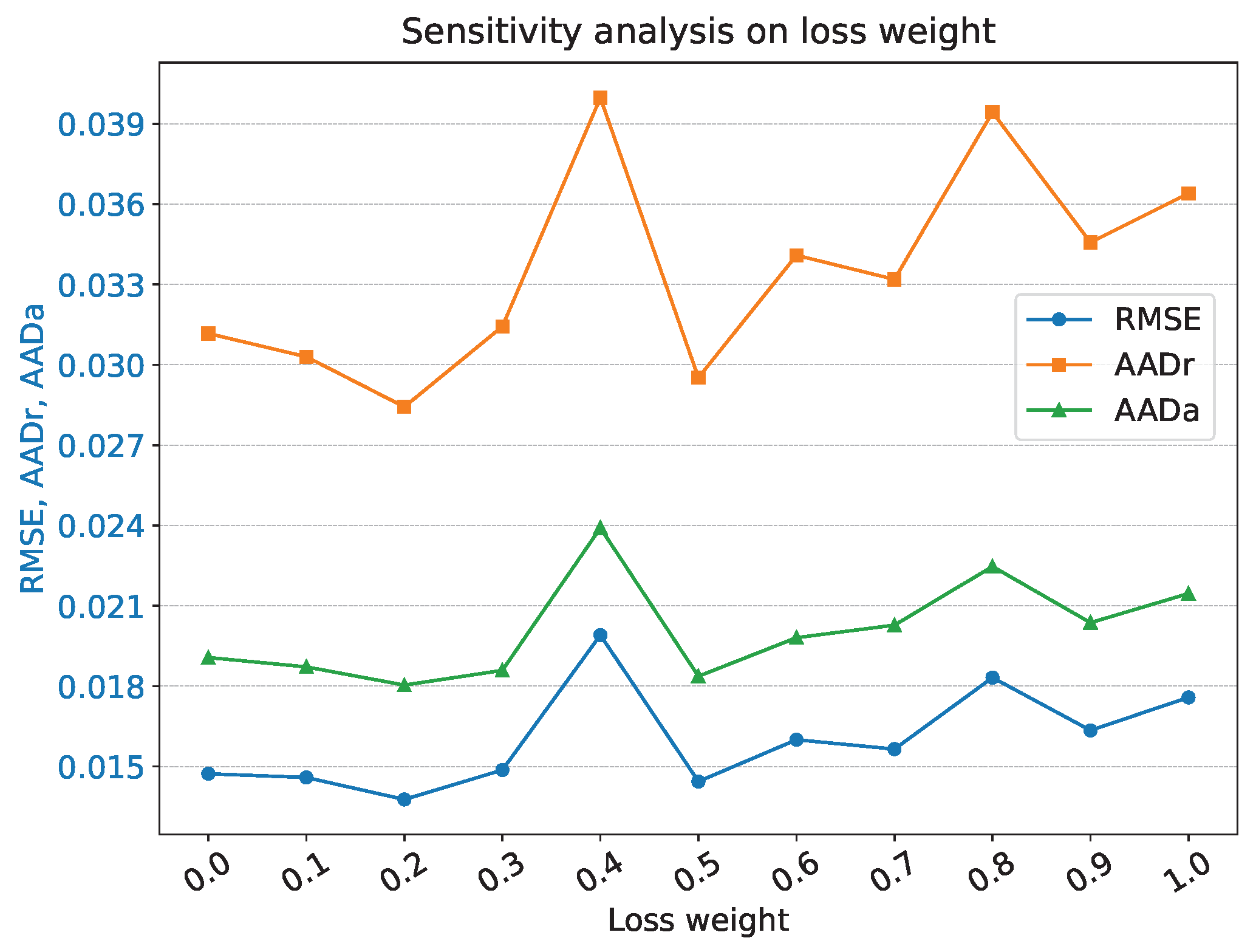
4.3.5. Weight of Loss
4.3.6. Running Time
5. Conclusions
Author Contributions
Funding
Data Availability Statement
Acknowledgments
Conflicts of Interest
References
- Chang, C.I. Hyperspectral Imaging: Techniques for Spectral Detection and Classification; Springer Science & Business Media: Berlin, Germany, 2003; Volume 1. [Google Scholar]
- Landgrebe, D. Hyperspectral image data analysis. IEEE Signal Process. Mag. 2002, 19, 17–28. [Google Scholar] [CrossRef]
- Li, H.; Lin, Z.; Ma, T.; Zhao, X.; Plaza, A.; William, J. Hybrid Fully Connected Tensorized Compression Network for Hyperspectral Image Classification. IEEE Trans. Geosci. Remote Sens. 2023, 61, 1–16. [Google Scholar] [CrossRef]
- Li, H.; Hu, W.; Li, W.; Li, J.; Du, Q.; Plaza, A. A3 CLNN: Spatial, Spectral and Multiscale Attention ConvLSTM Neural Network for Multisource Remote Sensing Data Classification. IEEE Trans. Neural Netw. Learn. Syst. 2020, 33, 747–761. [Google Scholar] [CrossRef] [PubMed]
- Lee, H.; Kwon, H. Going deeper with contextual CNN for hyperspectral image classification. IEEE Trans. Image Process. 2017, 26, 4843–4855. [Google Scholar] [CrossRef] [PubMed]
- Chang, C.I. Hyperspectral Data Exploitation: Theory and Applications; John Wiley & Sons: Hoboken, NJ, USA, 2007. [Google Scholar]
- Pistellato, M.; Bergamasco, F.; Torsello, A.; Barbariol, F.; Yoo, J.; Jeong, J.Y.; Benetazzo, A. A physics-driven CNN model for real-time sea waves 3D reconstruction. Remote Sens. 2021, 13, 3780. [Google Scholar] [CrossRef]
- Wang, L.; Chang, C.I.; Lee, L.C.; Wang, Y.; Xue, B.; Song, M.; Yu, C.; Li, S. Band subset selection for anomaly detection in hyperspectral imagery. IEEE Trans. Geosci. Remote Sens. 2017, 55, 4887–4898. [Google Scholar] [CrossRef]
- Plaza, A.; Benediktsson, J.A.; Boardman, J.W.; Brazile, J.; Bruzzone, L.; Camps-Valls, G.; Chanussot, J.; Fauvel, M.; Gamba, P.; Gualtieri, A.; et al. Recent advances in techniques for hyperspectral image processing. Remote Sens. Environ. 2009, 113, S110–S122. [Google Scholar] [CrossRef]
- Zhu, M.; Jiao, L.; Liu, F.; Yang, S.; Wang, J. Residual spectral–spatial attention network for hyperspectral image classification. IEEE Trans. Geosci. Remote Sens. 2020, 59, 449–462. [Google Scholar] [CrossRef]
- Pistellato, M.; Traviglia, A.; Bergamasco, F. Geolocating time: Digitisation and reverse engineering of a roman sundial. In Proceedings of the European Conference on Computer Vision, Glasgow, UK, 23–28 August 2 2020; pp. 143–158. [Google Scholar]
- Gong, M.; Zhang, M.; Yuan, Y. Unsupervised band selection based on evolutionary multiobjective optimization for hyperspectral images. IEEE Trans. Geosci. Remote Sens. 2015, 54, 544–557. [Google Scholar] [CrossRef]
- Ghamisi, P.; Yokoya, N.; Li, J.; Liao, W.; Liu, S.; Plaza, J.; Rasti, B.; Plaza, A. Advances in hyperspectral image and signal processing: A comprehensive overview of the state of the art. IEEE Geosci. Remote Sens. Mag. 2017, 5, 37–78. [Google Scholar] [CrossRef]
- Li, S.; Song, W.; Fang, L.; Chen, Y.; Ghamisi, P.; Benediktsson, J.A. Deep learning for hyperspectral image classification: An overview. IEEE Trans. Geosci. Remote Sens. 2019, 57, 6690–6709. [Google Scholar] [CrossRef]
- Bioucas-Dias, J.; Plaza, A.; Dobigeon, N.; Parente, M.; Du, Q.; Gader, P.; Chanussot, J. Hyperspectral unmixing overview: Geometrical, statistical, and sparse regression-based approaches. IEEE J. Sel. Top. Appl. Earth Observ. Remote Sens. 2012, 5, 354–379. [Google Scholar] [CrossRef]
- Feng, X.; Li, H.; Wang, R.; Du, Q.; Jia, X.; Plaza, A. Hyperspectral unmixing based on nonnegative matrix factorization: A comprehensive review. IEEE J. Sel. Top. Appl. Earth Observ. Remote Sens. 2022, 15, 4414–4436. [Google Scholar] [CrossRef]
- Bhatt, J.; Joshi, M. Deep learning in hyperspectral unmixing: A review. In Proceedings of the IGARSS 2020-2020 IEEE International Geoscience and Remote Sensing Symposium, Waikoloa, HI, USA, 26 September–2 October 2020; pp. 2189–2192. [Google Scholar]
- Chen, J.; Zhao, M.; Wang, X.; Richard, C.; Rahardja, S. Integration of physics-based and data-driven models for hyperspectral image unmixing: A summary of current methods. IEEE Signal Process. Mag. 2023, 40, 61–74. [Google Scholar] [CrossRef]
- Borsoi, R.; Imbiriba, T.; Bermudez, J.; Richard, C.; Chanussot, J.; Drumetz, L.; Tourneret, J.; Zare, A.; Jutten, C. Spectral variability in hyperspectral data unmixing: A comprehensive review. IEEE Geosci. Remote Sens. Mag. 2021, 9, 223–270. [Google Scholar] [CrossRef]
- Li, H.; Feng, X.; Zhai, D.; Du, Q.; Plaza, A. Self-supervised robust deep matrix factorization for hyperspectral unmixing. IEEE Trans. Geosci. Remote Sens. 2021, 60, 5513214. [Google Scholar] [CrossRef]
- Hong, D.; Gao, L.; Yao, J.; Yokoya, N.; Chanussot, J.; Heiden, U.; Zhang, B. Endmember-guided unmixing network (EGU-Net): A general deep learning framework for self-supervised hyperspectral unmixing. IEEE Trans. Neural Netw. Learn. Syst. 2021, 33, 6518–6531. [Google Scholar] [CrossRef]
- Jin, Q.; Ma, Y.; Fan, F.; Huang, J.; Mei, X.; Ma, J. Adversarial autoencoder network for hyperspectral unmixing. IEEE Trans. Neural Netw. Learn. Syst. 2023, 34, 4555–4569. [Google Scholar] [CrossRef]
- Rasti, B.; Koirala, B.; Scheunders, P.; Ghamisi, P. UnDIP: Hyperspectral unmixing using deep image prior. IEEE Trans. Geosci. Remote Sens. 2021, 60, 5504615. [Google Scholar] [CrossRef]
- Zhao, M.; Wang, M.; Chen, J.; Rahardja, S. Hyperspectral unmixing for additive nonlinear models with a 3-D-CNN autoencoder network. IEEE Trans. Geosci. Remote Sens. 2021, 60, 5509415. [Google Scholar] [CrossRef]
- Su, Y.; Li, J.; Plaza, A.; Marinoni, A.; Gamba, P.; Chakravortty, S. DAEN: Deep autoencoder networks for hyperspectral unmixing. IEEE Trans. Geosci. Remote Sens. 2019, 57, 4309–4321. [Google Scholar] [CrossRef]
- Su, Y.; Xu, X.; Li, J.; Qi, H.; Gamba, P.; Plaza, A. Deep autoencoders with multitask learning for bilinear hyperspectral unmixing. IEEE Trans. Geosci. Remote Sens. 2020, 59, 8615–8629. [Google Scholar] [CrossRef]
- Palsson, B.; Sigurdsson, J.; Sveinsson, J.R.; Ulfarsson, M.O. Hyperspectral unmixing using a neural network autoencoder. IEEE Access 2018, 6, 25646–25656. [Google Scholar] [CrossRef]
- Su, Y.; Marinoni, A.; Li, J.; Plaza, J.; Gamba, P. Stacked nonnegative sparse autoencoders for robust hyperspectral unmixing. IEEE Geosci. Remote Sens. Lett. 2018, 15, 1427–1431. [Google Scholar] [CrossRef]
- Ghosh, P.; Roy, S.K.; Koirala, B.; Rasti, B.; Scheunders, P. Hyperspectral unmixing using transformer network. IEEE Trans. Geosci. Remote Sens. 2022, 60, 5535116. [Google Scholar] [CrossRef]
- Zhao, M.; Shi, S.; Chen, J.; Dobigeon, N. A 3-D-CNN framework for hyperspectral unmixing with spectral variability. IEEE Trans. Geosci. Remote Sens. 2022, 60, 5521914. [Google Scholar] [CrossRef]
- Zhao, M.; Yan, L.; Chen, J. LSTM-DNN based autoencoder network for nonlinear hyperspectral image unmixing. IEEE J. Sel. Top. Signal Process. 2021, 15, 295–309. [Google Scholar] [CrossRef]
- Zhang, X.; Sun, Y.; Zhang, J.; Wu, P.; Jiao, L. Hyperspectral unmixing via deep convolutional neural networks. IEEE Geosci. Remote Sens. Lett. 2018, 15, 1755–1759. [Google Scholar] [CrossRef]
- Tao, X.; Paoletti, M.E.; Han, L.; Wu, Z.; Ren, P.; Plaza, J.; Plaza, A.; Haut, J.M. A new deep convolutional network for effective hyperspectral unmixing. IEEE J. Sel. Top. Appl. Earth Observ. Remote Sens. 2022, 15, 6999–7012. [Google Scholar] [CrossRef]
- Zou, L.; Zhu, X.; Wu, C.; Liu, Y.; Qu, L. Spectral–spatial exploration for hyperspectral image classification via the fusion of fully convolutional networks. IEEE J. Sel. Top. Appl. Earth Observ. Remote Sens. 2020, 13, 659–674. [Google Scholar] [CrossRef]
- Nalepa, J.; Myller, M.; Kawulok, M. Validating hyperspectral image segmentation. IEEE Geosci. Remote Sens. Lett. 2019, 16, 1264–1268. [Google Scholar] [CrossRef]
- Garcia-Garcia, A.; Orts-Escolano, S.; Oprea, S.; Villena-Martinez, V.; Garcia-Rodriguez, J. A review on deep learning techniques applied to semantic segmentation. arXiv 2017, arXiv:1704.06857. [Google Scholar]
- Guo, Y.; Liu, Y.; Georgiou, T.; Lew, M.S. A review of semantic segmentation using deep neural networks. Int. J. Multimedia Inf. Retr. 2018, 7, 87–93. [Google Scholar] [CrossRef]
- Mo, Y.; Wu, Y.; Yang, X.; Liu, F.; Liao, Y. Review the state-of-the-art technologies of semantic segmentation based on deep learning. Neurocomputing 2022, 493, 626–646. [Google Scholar] [CrossRef]
- Long, J.; Shelhamer, E.; Darrell, T. Fully convolutional networks for semantic segmentation. In Proceedings of the IEEE Conference on Computer Vision and Pattern Recognition, Boston, MA, USA, 7–12 June 2015; pp. 3431–3440. [Google Scholar]
- Qu, Y.; Qi, H. uDAS: An untied denoising autoencoder with sparsity for spectral unmixing. IEEE Trans. Geosci. Remote Sens. 2018, 57, 1698–1712. [Google Scholar] [CrossRef]
- Zhao, M.; Wang, X.; Chen, J.; Chen, W. A plug-and-play priors framework for hyperspectral unmixing. IEEE Trans. Geosci. Remote Sens. 2021, 60, 5501213. [Google Scholar] [CrossRef]
- Palsson, B.; Ulfarsson, M.O.; Sveinsson, J.R. Convolutional autoencoder for spectral–spatial hyperspectral unmixing. IEEE Trans. Geosci. Remote Sens. 2020, 59, 535–549. [Google Scholar] [CrossRef]
- Wang, M.; Zhao, M.; Chen, J.; Rahardja, S. Nonlinear unmixing of hyperspectral data via deep autoencoder networks. IEEE Geosci. Remote Sens. Lett. 2019, 16, 1467–1471. [Google Scholar] [CrossRef]
- Shahid, K.T.; Schizas, I.D. Unsupervised hyperspectral unmixing via nonlinear autoencoders. IEEE Trans. Geosci. Remote Sens. 2021, 60, 5506513. [Google Scholar] [CrossRef]
- Shi, S.; Zhao, M.; Zhang, L.; Altmann, Y.; Chen, J. Probabilistic generative model for hyperspectral unmixing accounting for endmember variability. IEEE Trans. Geosci. Remote Sens. 2021, 60, 5516915. [Google Scholar] [CrossRef]
- Borsoi, R.A.; Imbiriba, T.; Bermudez, J.C.M. Deep generative endmember modeling: An application to unsupervised spectral unmixing. IEEE Trans. Comput. Imaging 2019, 6, 374–384. [Google Scholar] [CrossRef]
- Han, Z.; Hong, D.; Gao, L.; Zhang, B.; Chanussot, J. Deep half-siamese networks for hyperspectral unmixing. IEEE Geosci. Remote Sens. Lett. 2020, 18, 1996–2000. [Google Scholar] [CrossRef]
- Zhou, C.; Rodrigues, M.R. ADMM-based hyperspectral unmixing networks for abundance and endmember estimation. IEEE Trans. Geosci. Remote Sens. 2021, 60, 5520018. [Google Scholar] [CrossRef]
- Zhang, J.; Zhang, X.; Tang, X.; Chen, P.; Jiao, L. Sketch-based region adaptive sparse unmixing applied to hyperspectral image. IEEE Trans. Geosci. Remote Sens. 2020, 58, 8840–8856. [Google Scholar] [CrossRef]
- Xiong, F.; Zhou, J.; Tao, S.; Lu, J.; Qian, Y. SNMF-Net: Learning a deep alternating neural network for hyperspectral unmixing. IEEE Trans. Geosci. Remote Sens. 2021, 60, 5510816. [Google Scholar] [CrossRef]
- Feng, X.R.; Li, H.C.; Liu, S.; Zhang, H. Correntropy-based autoencoder-like NMF with total variation for hyperspectral unmixing. IEEE Geosci. Remote Sens. Lett. 2020, 19, 5500505. [Google Scholar]
- Zhang, S.; Li, J.; Li, H.C.; Deng, C.; Plaza, A. Spectral–spatial weighted sparse regression for hyperspectral image unmixing. IEEE Trans. Geosci. Remote Sens. 2018, 56, 3265–3276. [Google Scholar] [CrossRef]
- Min, A.; Guo, Z.; Li, H.; Peng, J. JMnet: Joint metric neural network for hyperspectral unmixing. IEEE Trans. Geosci. Remote Sens. 2021, 60, 5505412. [Google Scholar] [CrossRef]
- Palsson, B.; Sveinsson, J.R.; Ulfarsson, M.O. Blind hyperspectral unmixing using autoencoders: A critical comparison. IEEE J. Sel. Top. Appl. Earth Observ. Remote Sens. 2022, 15, 1340–1372. [Google Scholar] [CrossRef]
- Ozkan, S.; Kaya, B.; Akar, G.B. Endnet: Sparse autoencoder network for endmember extraction and hyperspectral unmixing. IEEE Trans. Geosci. Remote Sens. 2018, 57, 482–496. [Google Scholar] [CrossRef]
- Qian, Y.; Xiong, F.; Qian, Q.; Zhou, J. Spectral mixture model inspired network architectures for hyperspectral unmixing. IEEE Trans. Geosci. Remote Sens. 2020, 58, 7418–7434. [Google Scholar] [CrossRef]
- Khajehrayeni, F.; Ghassemian, H. Hyperspectral unmixing using deep convolutional autoencoders in a supervised scenario. IEEE J. Sel. Top. Appl. Earth Observ. Remote Sens. 2020, 13, 567–576. [Google Scholar] [CrossRef]
- Yang, B. Supervised nonlinear hyperspectral unmixing with automatic shadow compensation using multiswarm particle swarm optimization. IEEE Trans. Geosci. Remote Sens. 2022, 60, 5529618. [Google Scholar] [CrossRef]
- Xu, X.; Shi, Z.; Pan, B. A supervised abundance estimation method for hyperspectral unmixing. Remote Sens. Lett. 2018, 9, 383–392. [Google Scholar] [CrossRef]
- Li, J.; Li, X.; Huang, B.; Zhao, L. Hopfield neural network approach for supervised nonlinear spectral unmixing. IEEE Geosci. Remote Sens. Lett. 2016, 13, 1002–1006. [Google Scholar] [CrossRef]
- Wan, L.; Chen, T.; Plaza, A.; Cai, H. Hyperspectral unmixing based on spectral and sparse deep convolutional neural networks. IEEE J. Sel. Top. Appl. Earth Observ. Remote Sens. 2021, 14, 11669–11682. [Google Scholar] [CrossRef]
- Altmann, Y.; Halimi, A.; Dobigeon, N.; Tourneret, J.Y. Supervised nonlinear spectral unmixing using a polynomial post nonlinear model for hyperspectral imagery. In Proceedings of the 2011 IEEE International Conference on Acoustics, Speech and Signal Processing (ICASSP), Prague, Czech Republic, 22–27 May 2011; pp. 1009–1012. [Google Scholar]
- Koirala, B.; Khodadadzadeh, M.; Contreras, C.; Zahiri, Z.; Gloaguen, R.; Scheunders, P. A supervised method for nonlinear hyperspectral unmixing. Remote Sens. 2019, 11, 2458. [Google Scholar] [CrossRef]
- Lei, M.; Li, J.; Qi, L.; Wang, Y.; Gao, X. Hyperspectral Unmixing via Recurrent Neural Network With Chain Classifier. In Proceedings of the IGARSS 2020-2020 IEEE International Geoscience and Remote Sensing Symposium, Waikoloa, HI, USA, 26 September–2 October 2020; pp. 2173–2176. [Google Scholar]
- Mitraka, Z.; Del Frate, F.; Carbone, F. Nonlinear spectral unmixing of landsat imagery for urban surface cover mapping. IEEE J. Sel. Top. Appl. Earth Observ. Remote Sens. 2016, 9, 3340–3350. [Google Scholar] [CrossRef]
- Hu, J.; Shen, L.; Sun, G. Squeeze-and-excitation networks. In Proceedings of the IEEE Conference on Computer Vision and Pattern Recognition, Salt Lake City, UT, USA, 18–23 June 2018; pp. 7132–7141. [Google Scholar]
- Wang, Q.; Wu, B.; Zhu, P.; Li, P.; Zuo, W.; Hu, Q. ECA-Net: Efficient channel attention for deep convolutional neural networks. In Proceedings of the IEEE/CVF Conference on Computer Vision and Pattern Recognition, Seattle, WA, USA, 13–19 June 2020; pp. 11534–11542. [Google Scholar]
- Woo, S.; Park, J.; Lee, J.Y.; Kweon, I.S. Cbam: Convolutional block attention module. In Proceedings of the European Conference on Computer Vision (ECCV), Munich, Germany, 8–14 September 2018; pp. 3–19. [Google Scholar]


| Blocks | Configurations | |||
|---|---|---|---|---|
| Output Size | Kernel Size | Stride | Padding | |
| Input | (32, B a, I b, I) | (3, 3) | (1, 1) | (1, 1) |
| Bands reduction | (32, 64, I, I) | (3, 3) | (1, 1) | (1, 1) |
| Conv1 | (32, 64, I, I) | (3, 3) | (1, 1) | (1, 1) |
| Pool1 c | (32, 64, I/2, I/2) | (2, 2) | (2, 2) | (0, 0) |
| Conv2 | (32, 128, I/2, I/2) | (3, 3) | (1, 1) | (1, 1) |
| Pool2 | (32, 128, I/4, I/4) | (2, 2) | (2, 2) | (0, 0) |
| Conv3 | (32, 256, I/4, I/4) | (3, 3) | (1, 1) | (1, 1) |
| ConvTransp1 d | (32, 128, I/2, I/2) | (2, 2) | (2, 2) | (0, 0) |
| Replication1 e | (32, 128, I/2, I/2) | - | - | - |
| ConvTransp2 | (32, 64, I, I) | (2, 2) | (2, 2) | (0, 0) |
| Spatial–spectral attention module | (32, 64, I, I) | - | - | - |
| Replication2 | (32, 64, I, I) | - | - | - |
| Conv4 | (32, P f, I, I) | (3, 3) | (1, 1) | (1, 1) |
| Abundance constraint module | (32, P, I, I) | - | - | - |
| Softplus | (32, P, I, I) | - | - | - |
| ASC g | (32, P, I, I) | - | - | - |
| MaxPool1 h | (32, 64, 1, 1) | - | - | - |
| AvgPool1 | (32, 64, 1, 1) | - | - | - |
| Conv5 | (32, 4, 1, 1) | (1, 1) | (0, 0) | (0, 0) |
| Conv6 | (32, 64, 1, 1) | (1, 1) | (0, 0) | (0, 0) |
| Sigmoid1 | (32, 64, 1, 1) | - | - | - |
| MaxPool2 | (32, 1, I, I) | - | - | - |
| AvgPool2 | (32, 1, I, I) | - | - | - |
| Concat | (32, 2, I, I) | - | - | - |
| Conv7 | (32, 1, I, I) | - | - | - |
| Sigmoid2 | (32, 1, I, I) | - | - | - |
| Hyperparameters | Values | Hyperparameters | Values |
|---|---|---|---|
| Epochs | 500 | Softplus threshold | 1.0 |
| Batch size | 32 | Patch size | 4 |
| Optimizer | Adam | Training set ratio | 0.2 |
| Learning rate | 0.01 | Validation set ratio | 0.1 |
| Learning rate scheduler | StepLR | Test set ratio | 0.7 |
| Scheduler step size | 50 | Augment times | 5 |
| Scheduler gamma | 0.8 | Loss weight | 0.2 |
| Metrics | Methods | ||||||
|---|---|---|---|---|---|---|---|
| VAEUN | DAEU | DeepTrans | CubeCNN | CrossCUN | PFSSA | ||
| #1 | noise-free | 0.0279 | 0.1327 | 0.1027 | 0.0677 | 0.1371 | 0.0184 |
| 20 dB | 0.0433 | 0.1167 | 0.0947 | 0.0548 | 0.1466 | 0.0292 | |
| #2 | noise-free | 0.0205 | 0.1341 | 0.0325 | 0.0667 | 0.1487 | 0.0119 |
| 20 dB | 0.0240 | 0.1242 | 0.0346 | 0.0542 | 0.1483 | 0.0181 | |
| #3 | noise-free | 0.0625 | 0.1966 | 0.2037 | 0.0400 | 0.1562 | 0.0256 |
| 20 dB | 0.0769 | 0.2632 | 0.1977 | 0.0395 | 0.1758 | 0.0364 | |
| #4 | noise-free | 0.0342 | 0.1137 | 0.0337 | 0.0458 | 0.1280 | 0.0135 |
| 20 dB | 0.0276 | 0.1583 | 0.0389 | 0.0429 | 0.1443 | 0.0193 | |
| #5 | noise-free | 0.0538 | 0.1922 | 0.1128 | 0.0470 | 0.1910 | 0.0197 |
| 20 dB | 0.0519 | 0.2456 | 0.1189 | 0.0438 | 0.2007 | 0.0330 | |
| noise-free | 0.0428 | 0.1576 | 0.1157 | 0.0548 | 0.1561 | 0.0187 | |
| 20 dB | 0.0486 | 0.1917 | 0.1139 | 0.0476 | 0.1678 | 0.0283 | |
| noise-free | 0.0924 | 0.4590 | 0.4159 | 0.1178 | 0.2881 | 0.0580 | |
| 20 dB | 0.1476 | 0.5759 | 0.4062 | 0.1070 | 0.3427 | 0.0847 | |
| noise-free | 0.0791 | 0.3769 | 0.2272 | 0.1127 | 0.2302 | 0.0335 | |
| 20 dB | 0.1195 | 0.3737 | 0.2289 | 0.1004 | 0.2532 | 0.0583 | |
| Metrics | Methods | ||||||
|---|---|---|---|---|---|---|---|
| VAEUN | DAEU | DeepTrans | CubeCNN | CrossCUN | PFSSA | ||
| Soil | 0.2615 | 0.0914 | 0.1773 | 0.0440 | 0.1792 | 0.0183 | |
| Tree | 0.2697 | 0.0786 | 0.2007 | 0.0381 | 0.1631 | 0.0148 | |
| Water | 0.4027 | 0.0386 | 0.3100 | 0.0236 | 0.0831 | 0.0108 | |
| 0.3180 | 0.0731 | 0.2365 | 0.0363 | 0.1487 | 0.0149 | ||
| 0.7054 | 0.1530 | 0.5332 | 0.0685 | 0.2722 | 0.0338 | ||
| 0.5923 | 0.1014 | 0.3940 | 0.0544 | 0.1879 | 0.0197 | ||
| Metrics | Methods | ||||||
|---|---|---|---|---|---|---|---|
| VAEUN | DAEU | DeepTrans | CubeCNN | CrossCUN | PFSSA | ||
| Tree | 0.1557 | 0.1106 | 0.0828 | 0.0394 | 0.2370 | 0.0245 | |
| Water | 0.2145 | 0.1638 | 0.1919 | 0.0250 | 0.0764 | 0.0304 | |
| Soil | 0.1809 | 0.1632 | 0.2052 | 0.0476 | 0.2359 | 0.0348 | |
| Road | 0.0771 | 0.2658 | 0.2863 | 0.0377 | 0.1437 | 0.0391 | |
| 0.1650 | 0.1846 | 0.2048 | 0.0385 | 0.1880 | 0.0328 | ||
| 0.4164 | 0.4527 | 0.4971 | 0.0904 | 0.4275 | 0.0887 | ||
| 0.3290 | 0.3247 | 0.3370 | 0.0646 | 0.2813 | 0.0402 | ||
| Metrics | Methods | ||||||
|---|---|---|---|---|---|---|---|
| VAEUN | DAEU | DeepTrans | CubeCNN | CrossCUN | PFSSA | ||
| Asphalt | 0.4087 | 0.2024 | 0.1583 | 0.0399 | 0.2053 | 0.0071 | |
| Grass | 0.3368 | 0.1405 | 0.1860 | 0.0464 | 0.2227 | 0.0081 | |
| Tree | 0.2655 | 0.0866 | 0.1300 | 0.0375 | 0.1881 | 0.0059 | |
| Roof | 0.1857 | 0.1167 | 0.1524 | 0.0277 | 0.1295 | 0.0062 | |
| 0.3104 | 0.1430 | 0.1579 | 0.0386 | 0.1920 | 0.0070 | ||
| 0.8406 | 0.3234 | 0.3833 | 0.0970 | 0.4319 | 0.0171 | ||
| 0.7399 | 0.2483 | 0.3610 | 0.0755 | 0.3288 | 0.0102 | ||
| Padding Mode | Metrics | ||||||
|---|---|---|---|---|---|---|---|
| Constant zeros | (0, 0, 1, 1) | 0.0221 | 0.0197 | 0.0154 | 0.0194 | 0.0447 | 0.0240 |
| (0, 1, 1, 0) | 0.0206 | 0.0165 | 0.0123 | 0.0168 | 0.0376 | 0.0222 | |
| (1, 0, 0, 1) | 0.0253 | 0.0221 | 0.0150 | 0.0213 | 0.0485 | 0.0269 | |
| (1, 1, 0, 0) | 0.0188 | 0.0163 | 0.0110 | 0.0157 | 0.0349 | 0.0208 | |
| Constant 0.5 | (0, 0, 1, 1) | 0.0265 | 0.0212 | 0.0257 | 0.0250 | 0.0557 | 0.0260 |
| (0, 1, 1, 0) | 0.0235 | 0.0178 | 0.0152 | 0.0194 | 0.0421 | 0.0227 | |
| (1, 0, 0, 1) | 0.0231 | 0.0208 | 0.0147 | 0.0199 | 0.0442 | 0.0238 | |
| (1, 1, 0, 0) | - a | - | - | - | - | - | |
| Constant ones | (0, 0, 1, 1) | 0.0277 | 0.0286 | 0.0267 | 0.0280 | 0.0631 | 0.0315 |
| (0, 1, 1, 0) | 0.0352 | 0.0251 | 0.0279 | 0.0301 | 0.0645 | 0.0317 | |
| (1, 0, 0, 1) | 0.0280 | 0.0250 | 0.0187 | 0.0243 | 0.0555 | 0.0293 | |
| (1, 1, 0, 0) | 0.0235 | 0.0249 | 0.0169 | 0.0222 | 0.0498 | 0.0239 | |
| Edge replicate | (0, 0, 1, 1) | 0.0191 | 0.0159 | 0.0108 | 0.0157 | 0.0360 | 0.0199 |
| (0, 1, 1, 0) | 0.0183 | 0.0148 | 0.0108 | 0.0149 | 0.0338 | 0.0197 | |
| (1, 0, 0, 1) | 0.0189 | 0.0167 | 0.0119 | 0.0161 | 0.0365 | 0.0210 | |
| (1, 1, 0, 0) | 0.0202 | 0.0167 | 0.0127 | 0.0169 | 0.0381 | 0.0213 | |
| Methods | VAEUN | DAEU | DeepTrans | CubeCNN | CrossCUN | PFSSA |
|---|---|---|---|---|---|---|
| Time (s) | 363.23 | 484.20 | 33.21 | 5973.32 | 12573.74 | 213.95 |
Disclaimer/Publisher’s Note: The statements, opinions and data contained in all publications are solely those of the individual author(s) and contributor(s) and not of MDPI and/or the editor(s). MDPI and/or the editor(s) disclaim responsibility for any injury to people or property resulting from any ideas, methods, instructions or products referred to in the content. |
© 2023 by the authors. Licensee MDPI, Basel, Switzerland. This article is an open access article distributed under the terms and conditions of the Creative Commons Attribution (CC BY) license (https://creativecommons.org/licenses/by/4.0/).
Share and Cite
Huang, J.; Zhang, P. Beyond Pixel-Wise Unmixing: Spatial–Spectral Attention Fully Convolutional Networks for Abundance Estimation. Remote Sens. 2023, 15, 5694. https://doi.org/10.3390/rs15245694
Huang J, Zhang P. Beyond Pixel-Wise Unmixing: Spatial–Spectral Attention Fully Convolutional Networks for Abundance Estimation. Remote Sensing. 2023; 15(24):5694. https://doi.org/10.3390/rs15245694
Chicago/Turabian StyleHuang, Jiaxiang, and Puzhao Zhang. 2023. "Beyond Pixel-Wise Unmixing: Spatial–Spectral Attention Fully Convolutional Networks for Abundance Estimation" Remote Sensing 15, no. 24: 5694. https://doi.org/10.3390/rs15245694
APA StyleHuang, J., & Zhang, P. (2023). Beyond Pixel-Wise Unmixing: Spatial–Spectral Attention Fully Convolutional Networks for Abundance Estimation. Remote Sensing, 15(24), 5694. https://doi.org/10.3390/rs15245694