Multi-Resolution Segmentation of Solar Photovoltaic Systems Using Deep Learning

Abstract

In the realm of solar photovoltaic system image segmentation, existing deep learning networks focus almost exclusively on single image sources both in terms of sensors used and image resolution. This often prevents the wide deployment of such networks. Our research introduces a novel approach to train a network on a diverse range of image data, spanning UAV, aerial, and satellite imagery at both native and aggregated resolutions of 0.1 m, 0.2 m, 0.3 m, 0.8 m, 1.6 m, and 3.2 m. Using extensive hyperparameter tuning, we first determined the best possible parameter combinations for the network based on the DeepLabV3 ResNet101 architecture. We then trained a model using the wide range of different image sources. The final network offers several advantages. It outperforms networks trained with single image sources in multiple test applications as measured by the F1-Score (95.27%) and IoU (91.04%). The network is also able to work with a variety of target imagery due to the fact that a diverse range of image data was used to train it. The model is made freely available for further applications.

1. Introduction

The expansion of renewable energies is of key importance for the future of energy supply. Numerous reasons speak to the need for this transformation and highlight the need for a transition from fossil fuels to sustainable energy sources. For example, access to clean energy plays a central role in improving the quality of life and protecting our environment [1]. In order to provide a solid basis for the management of the development and integration of renewable energies on a small local, national, and continental scale, the modeling of energy systems can be seen as a practical tool [2,3,4]. A large set of reliable input data is required to run such models. The data required depend on the specific energy management problem. In general, however, energy system models always require information on energy demand and energy production. If detailed information about the existing energy supply is not available for study areas, then machine learning (ML)-based methods of image recognition as well as earth-observation-based data offer a perspective for the generation of supplementary datasets.

The detection of existing renewable energy (RE) systems for mapping has been the goal of numerous studies [5]. While some early work on this topic deal with local spatial areas and individual PV systems [6], others generate datasets for entire countries [7]. Currently, from detailed local to global observations, various studies using remote sensing data such as satellite data [8,9], aerial images from aircraft [10,11], and drone images [12] exist to obtain detection at different scales in the respective study areas.

From published research in the field of PV system detection from images, it can be seen that there are numerous different ML methods used to perform the detection of PV systems. The meta-study “Advances and prospects on estimating solar photovoltaic (PV) installation capacity and potential based on satellite and aerial images” [13], for example, lists 17 different studies on the segmentation of PV systems in which different Fully Convolution Networks (FCN) and FCN-based methods are used. However, there are also numerous new studies with a strong focus on deep networks that are individually adapted to the task of segmenting PV systems. Zhu et al. [14] introduce a method to enhance PV segmentation from satellite imagery with a detail-oriented deep learning network using a Deeplabv3+ based Network. The network combines a Split-Attention Network and a Dual-Attention module with Atrous Spatial Pyramid Pooling (ASSP). Furthermore, the network has been proved to have favorable generalization capacity. Data from Google Earth Satellite with a resolution at 0.15 m in the area of Northern Baden-Württemberg in Germany was used to train the network. The authors also developed a new feature called the Constraint Refinement Module. The module enables the refinement tasks of localizing the PV panel region and thereby increasing the regulation of the PV panel shape [15]. Wang et al. [16] developed a size-aware deep-learning-based network for segmenting small-scale rooftop solar PV systems from high-resolution images. The size-aware network has performed well when it comes to the transfer of the application of the network to different datasets of similar pixel resolution.

While these studies achieve high accuracy, there is a notable caveat. The datasets used within this studies vary from 0.1 m to 30 m image resolution. Looking at the accuracy of the studies’ result metrics, it can be observed that the detection accuracy is very high regardless of the image resolution chosen. However, this is only the case as long as the image data of the training match the data of the validation as well as in the following real-life application. If trained networks are applied to new image data with a different image resolution, for example, this can lead to very poor accuracy without further training [17]. This leads to the models only be restrictively used in practice, which is a considerable disadvantage. In addition, care should be taken when combining image data from different sources such as Microsoft Bing Maps and Google Earth Engine (GEE). This is particularly true when using very-high-resolution (VHR) aerial and satellite imagery. This is due to the fact that the maximum resolution of images varies from region to region due to vastly uneven global availability [18]. Furthermore, distortions become apparent in certain areas such as the USA, Europe, and India with significant interference at political borders [19]. Therefore, in order to address the different requirements for such a PV system segmentation model, some studies have already partially investigated the suitability of combining different resolution datasets for training different methods. For example, Jiang et al. [17] investigated the suitability of “cross application at different resolutions” where models were trained with data of a specific native resolution and a subsequent test application was applied to image data of a different resolution. The results show very poor transferability. Conversely, the transfer of models from one to another native resolution can be done with very good results if networks are fine-tuned with the target resolution. However, this means that the accurate application to new image data basically requires fine-tuning of existing models to new image data. Su et al. [20] propose a cross-scale acquisition method that combines satellite data from the GaoFen constellation at 2 m resolution, Sentinel-2 at 10 m resolution, and Google satellite imagery aggregates at approximately 2 m and 10 m resolution. The results indicate that models can benefit from training with image data of different resolutions. Wang et al. [21] were recently able to show by enriching another external training data that enrichment with additional samples can lead to an increase in performance. Guo et al. [22] developed a deep learning model called GenPV. GenPV goes a step further by making use of unbalanced datasets using three-band red, green, blue (RGB) Google Earth tiles with a spatial resolution of 0.15, 0.3, and 0.6 m, respectively. The authors succeed in showing that a network trained with a single resolution can be transferred to another resolution with a high degree of performance [22].

Since, to the best of our knowledge, there is no research conducted that presents a model of PV segmentation that uses a variety of different image data with different resolutions and sensors for training at the same time, the effect of diverse image data on performance will be examined in more detail in this paper. Contrary to existing studies, this paper will not present an individualized deep-learning-based design. The focus is on successively enriching and combining a model with a large number of different existing training data by using the already extensively applied DeepLabV3 ResNet101 network. For this purpose, both native and aggregated images of the visible spectrum and resolutions in the range of 0.1 m, 0.2 m, 0.3 m, 0.8 m, 1.6 m, and 3.2 m as well as different sensor types of drone, aerial, and satellite images are used in this work. For comparison, the enriched networks are presented alongside models that were only trained on individual resolutions. Thus, this paper aims to describe the development of an image segmentation model capable of predicting PV systems from a variety of different images at different resolutions with a high level of performance.

2. Materials

In the domain of RS, a large number of different datasets have been published in recent years that can be used to train ML methods for detection of PV systems. These datasets can basically be distinguished into two different formats: vector and raster as training data in combination with aerial or satellite imagery. For example, Kruitwagen et al. [9] provide a dataset of large PV systems distributed across the globe. Dunnett et al. [23] even extend such a dataset with additional location data for wind generation facilities. However, image data are not included in these datasets. Conversely, the raster datasets are PV systems location data in the form of ready-made masks that are available along with image data collections. Therefore, the raster datasets can be used directly for training ML-based methods. All the datasets listed here have been manually inspected and tagged by humans. The first dataset mentioned here (

Table 1. Summary of the information on the various datasets.

Dataset	Sensor	Category	Resolution in m	Size in Pixel	Images with PV	Located	Publisher
DOP	Areal Image	Rooftop, Ground	0.1	320 × 320	2117	Germany	[10]
PV01	UAV	Rooftop	0.1	256 × 256	645	Hai’an/China	[17]
GEE	aggregated	Rooftop	0.1	400 × 400	13,303	France/Western Europe	[24]
IGN	Areal Image	Rooftop	0.2	400 × 400	7686	France	[24]
PV03	Areal Image	Rooftop, Ground	0.3	1024 × 1024	2308	Jiangsu China	[17]
PV08	GaoFen/Beijing-2	Rooftop, Ground	0.8	1024 × 1024	763	China	[17]

, dataset DOP) consists of aerial photographs from the Federal Agency for Cartography and Geodesy (BKG) in Germany covering the state of North Rhine-Westphalia with a native resolution of 0.1 m [10]. Other datasets used consist of image data located within China that were obtained from unmanned aerial vehicles (UAVs) in Hai’an county (Table 1, dataset PV01), area imagery from the Provincial Geomatics Center (PGC) of Jiangsu (Table 1, dataset PV03), and satellite imagery from Gaofen-2 as well as Beijing-2 satellite imagery (Table 1, dataset PV08) at resolutions of 0.1 m, 0.3 m, and 0.8 m, respectively, with masks of existing PV systems [17]. The most recent published dataset [24] consist of combinations of imagery data. The combine dataset contains overflight imagery in France from the National Institute of Geographic and Forest Information (IGN) Geoservices portal with a native resolution of 0.2 m (Table 1, dataset IGN) as well as images gathered using GEE with 0.1 m (Table 1, dataset GEE) native resolution around different places in Germany. A special feature of the latter dataset is that it contains locations in the form of masks of existing PV systems as well as other information such as roof slope and orientation. An overview of the essential data such as native resolutions, number of images, and sensors used can be found in Table 1.

3. Methods

The following section first describes the image data preprocessing. Subsequently, the model used, the training with different image datasets, the hyperparameter tuning, and finally, the steps of the validation are described.

3.1. Data Preprocessing

Preliminarily, six different resolution levels of 0.1 m (PV10), 0.2 m (PV20), 0.3 m (PV30), 0.8 m (PV80), 1.60 m (PV160), and 3.20 m (PV320) were defined. These resolution levels are chosen for two reasons: the limitation of the highest resolution of 0.1 m per pixel of the available training data and on the common zoom level (which ranges from 16 to 20) of the processing of image data from Bing Maps or GEE of approx. 0.1 m to 3.2 m. With the goal of dividing the available image data into the six image resolution classes, several preparatory steps were taken to prepare the image datasets. For the image data of all image resolutions, a consistent folder structure for images and masks was created that allows a static subdivision of the images for training, validation, and test. All images and masks were converted to a consistent image format. Furthermore, all masks were converted to binary format. For the dataset PV08, the images and masks (size of 1024 × 1024 pixels) were adjusted into 16 frames (256 × 256). For the aggregated stages of 1.6 m resolution, the underlying images (1024 × 1024) were divided into four frames (512 × 512) and then, formatted to 256 × 256 images using the nearest neighbor up-sampling method. Images with 3.2 m resolution were generated by directly up-sampling the PV08 images of size 1024 × 1024 to 256 × 256 with the nearest neighbor method. Then, the prepared image data and their corresponding masks were divided into the Training, Validation, and Test static folders by random selection. Special consideration was given to the division of the resolution levels between 0.8 and 3.2 m because the image contents show the same scenes. To avoid overfitting, care was taken to ensure that the same image content was stored in the Training, Validation, and Test folders. To keep the amount of data manageable, the amount of data for the comparisons of single-resolution and multi-resolution as well as hyperparameter tuning was limited to 1000 images per resolution level in training and 100 images per resolution level for both validation and testing phases. Thus, approximately 83.3%, 8.3%, and 8.3% of the image data is available for training, validation, and testing, respectively. The ratio of counted pixels between existing solar PV systems and the background class varies greatly within the datasets. The ratios of each dataset are shown in

Table 2. Ratio of pixels containing solar PV systems per dataset.

Dataset	Percentage of Pixels Containing Solar PV Systems (%)
PV01	10.9
PV02	19.2
PV03	57.9
PV08	36.7
PV16	22.8
PV32	12.8

. Since several datasets with the same resolution were available, the images were combined and used for training. The only exception is the resolution level of 3.2 m with only 563 images in total in training because the whole dataset is limited to 763 images.

Examples of the final image data are shown in Figure 1. The final model was then trained with all available images with the exception of images for validation and testing.

3.2. Model

In choosing the model for the study, use was made of the existing DeepLabv3 network [25]. An essential key feature of the architecture is ASPP. ASPP is a DeepLab semantic segmentation module for resampling a given feature layer at multiple rates before convolution. The initial image is augmented with multiple filters of complementary effective fields of views. This allows objects as well as useful image context to be captured at multiple scales. A mapping strategy is implemented by using multiple parallel Atrous convolutional layers at different sampling rates instead of the resampling of features. Moreover, a spatial pyramid pooling (SPP) scheme is added. By using an SPP, parallel dilated convolutions with different rates can be applied to the input feature map. The feature map and dilated convolutions are then merged. Since objects of the same class can be represented at different sizes in the images used, ASPP can accommodate the different object sizes [26]. Finally, DeepLabv3 improves on previous versions of the model to deal with object segmentation problems at different scales. Modules have been developed to cascade or perform parallel Atrous convolutions to capture the context of multiple scales. For this purpose, several Atrous rates were introduced. Additionally, global context encoding has been added to the ASPP module, which further increases performance [25]. Combining DeepLabv3 with the deep residual neural network ResNet101 [27] as a backbone has repeatedly proven to be very effective for segmenting different image scenes [28,29,30]. Python 3.10, Torch 1.14.0, and Torchvision version 0.15.0 were all used for development of the model. Pre-trained weights from COCO “DeepLabV3 ResNet101 Weights COCO WITH VOC LABELS V1” were used for all training. Here, all models are evaluated with an independent test dataset that is included in the Pascal VOC dataset. The Pascal VOC dataset contains 20 categories. These weights were selected based on the performance indicated by the pixel accuracy of 92.4% as well as a mean Intersection over Union (IoU) of 67.4% on Torchvision v0.15 [31]. The segmentation model can be implemented by using a DeepLabV3 segmentation head that was set by integrating the ASPP module with an input channel of 2048 and different dilation rates (12, 24, and 36) to capture multi-scale context information. The number of model parameters is approx. 61 million and the Giga Floating Point Operations Per Second (GFLOPS) are 258.74.

3.3. Model Training

3.3.1. Hyperparameter Tuning

During hyperparameter tuning, a full grid search was applied in which all possible parameter combinations were tested.

Table 3. Hyperparameter search space metrics.

Hyperparameter	Search Range
Loss function	Huber loss, BCE loss, MSE loss, CE loss
Optimizer	Adagrad, Adam, RMSprop, SGD
Learning rate	0.001, 0.0001, 0.00001
Batch size	2, 4, 8, 12, 16, 24, 32, 48, 64
Stride	2, 3, 4, 5

shows the search space metrics of the grid search where four loss functions, four optimizers, three learning rates, nine batch sizes, and four stride values are defined. These parameters are chosen due to the fact that the selected combined model, DeepLabV3 ResNet101, uses pre-trained weights. Therefore, hyperparameters were selected such that the model is as fine-tuned as possible to perform image segmentation. Direct parameter changes were avoided to preserve the integrity of the pre-trained weights, which ensures that the advantage of what using said weights brings is maintained. Examples of direct parameters omitted from tuning are number of layers, pooling type, and activation function types. The goal is to tune the listed parameters available with pre-trained weights such that evaluation metrics are maximized.

The parameters’ loss function, optimizer, and learning rate were tested simultaneously. Conversely, batch size and stride parameters were tested independently and in isolation from other parameters. Additionally, an early stopping mechanism was utilized to prevent the model from overfitting to the training data. The mechanism involves evaluating the performance of model every 10 epochs using the IoU metric. The best IoU value would be checked every 10 epochs and if the IoU value for that epoch is greater than the current best IoU, then the IoU value for that particular epoch would then be the new benchmark value for future performance checks. However, if the opposite occurs where the current best IoU is greater than the IoU value for that epoch, then the model training is stopped. Lastly, a maximum of 100 epochs is used for training.

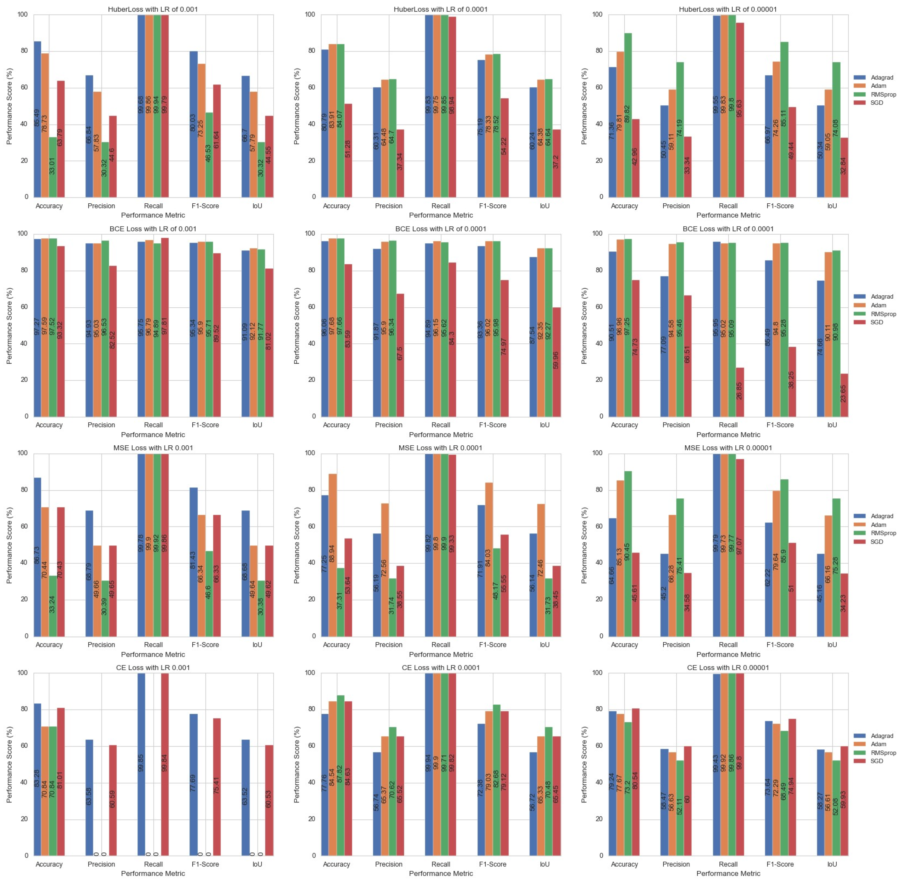
Four loss functions are selected for tuning. The Huber loss function, invented by Huber in 1964, provides robustness as it has duality in its behavior in how to treats outlier and inlier errors [32]. According to Huber, the function will apply the squared error function (L2 loss) for error values below a particular threshold. However, if the error value is above the threshold, a scaled absolute (L1 loss) error loss function would be applied [32]. This, therefore, means that the Huber loss function behaves like a piecewise function. The threshold is called the delta variable ($\delta$). The delta variable is the threshold for errors that are considered outliers. Furthermore, the Huber loss function is differentiable everywhere. When comparing different loss functions, it was concluded that dynamic loss functions (such as Huber loss) yielded better model performance during training regression CNN architecture [33]. Mathematically, the function can be described as follows:

$$Huberloss(y, f\left(x\right))=\left\{\begin{array}{cc}\frac{1}{2}{(y-f\left(x\right))}^2,\hfill & \mathrm{if}|y-f(x\left)\right|\le \delta \hfill \\ \delta \left(\right|y-f\left(x\right)|-\frac{1}{2}\delta ),\hfill & \mathrm{otherwise}\hfill \end{array}\right.$$

(1)

The Cross-Entropy loss (CE loss) function can be referred to as logarithmic loss. For a given set of predictions, the loss function simply averages the sum of the products of truth values (y) and the log of the predicted values (p) from the model.

$$CEloss(y, p)=-\sum _i{y}_{i}log\left(p_i\right)$$

(2)

Binary Cross-Entropy (BCE) loss is a specific variation of Cross-Entropy loss tailored for binary classification tasks, where there are only two possible classes (e.g., 0 and 1). Unlike the standard CE loss function, BCE loss calculates the error for predicting binary outcomes and is ideal for problems with binary class labels. The BCEWithLogits loss function is a combination of sigmoid and BCE loss and is numerically stable.

$$BCEWithLogitsloss(y, z)=-[y·log(\sigma \left(z\right))+(1-y)·log(1-\sigma \left(z\right)\left)\right]$$

(3)

Here, y is the true label, z represents the logit or the output of your model, and $\sigma$$\left(z\right)$ is the sigmoid function which converts the logits into probabilities. The BCE loss measures the difference between the predicted probabilities and the true labels. This loss function has been successfully implemented in applications such as video segmentation to minimize motion blur. Implementation involved using BCEWithLogits function in an UNet inspired encoder–decoder network [34]. Another study aimed to create a pix2pix Generative Adversarial Network (GAN) that can generate synthetic computerized tomography (sCT) images using positron emission tomography (PET) images [35]. The BCEWithLogits loss function was used for both the generator and discriminator of the GAN in combination with other loss functions. The last loss function tested is the Mean Squared Error (MSE) loss function:

$$MSEloss(y, f\left(x\right))=\frac{1}{n}\sum _{i=1}^n{(y_i-f\left(x_i\right))}^2$$

(4)

The MSE loss function is the squared difference between the ground truth (y) and prediction value ($f\left(x\right)$). Squaring the error helps the model penalize large errors. However, it should not be used with data with a sizable percentage of outliers for this reason.

The optimizers selected are the Adagrad, Adam, RMSProp, and SGD optimizers. The optimizer is responsible for backpropagation, whereby each weight is adjusted based on the error computed by the loss function. Due to backpropagation, each loss function must be differentiable as the derivative of it is found and used to adjust the weights. This means that the loss function is the objective function as it is the function that the optimizer is attempting to minimize its output. Weights are adjusted by finding the derivative of the loss function with respect to weight and subtracting that derivative value from the original weight value. To further increase the rate of the optimization to minimize the loss function’s output, the derivative value is multiplied by a factor so that the minimum is found more quickly. The multiplying factor is called the learning rate. This process continues until the minimum of the loss function is found, i.e., when the derivative of the loss function is zero and the weights can no longer be adjusted. This entire process is called Stochastic Gradient Descent (SGD). The Adagrad, Adam, and RMSProp optimizers are optimizers with adaptive learning rates. The Adaptive Gradient (Adagrad) optimizer implements an algorithm that controls proximal functions, which in turn modifies the “gradient steps of the algorithm” [36]. The study that introduced this approach concluded that adaptive optimizers’ algorithms outperform non-adaptive algorithms [36]. The Adagrad optimizer is known for its adaptive learning rate approach. It is, therefore, well-suited for scenarios where the characteristics of the solar PV systems in images may vary widely. Adagrad can effectively navigate complex and varied landscapes by adjusting the learning rates for each parameter individually based on their historical gradients. This can be the case with PV segmentation. The Root Mean Square Propagation (RMSProp) algorithm was used to optimize the weights in recurrent neural network (RNN) using Long Short-term Memory (LSTM) units [37]. The model was trained to generate text sequences for handwritten text. The model was successful at both generating text as well as handwriting styles. By finding the running average of recent gradients for a particular weight, the value of that weight can be adjusted by dividing it by that average [37]. RMSProp, like Adagrad, incorporates adaptive learning rates but it further addresses the diminishing learning rate problem. In the context of PV systems segmentation, certain features may require more nuanced adjustments during optimization. RMSProp’s ability could, therefore, be used to adaptively scale the learning rates for different parameters and lead to more efficient convergence. The Adaptive Moment Estimation (Adam) algorithm was introduced in 2014 by Kingma and Lei Ba [38]. It is a gradient-based stochastic optimization algorithm. This algorithm requires fewer computational resources and less memory and is relatively straightforward to implement [38]. Using the Adam optimization takes advantage of both the Adagrad and RMSProp methods. Sparse gradients and non-stationary objectives are resolved using the intricacies deployed in both the Adagrad and RMSProp methods, respectively, [38]. Computational resources and memory efficiency are critical in the context of using large amounts of data in PV segmentation. The capability of the Adam optimizer to provide effective optimization with reduced resource requirements makes it an attractive optimizer to consider. The last optimizer to be tested is the standard SGD algorithm. This algorithm is non-adaptive, meaning that the learning rate is static. Standard SGD is a fundamental optimizer that can serve as a basis for comparison. In particular, SGD proves to be a reliable option in PV segmentation since the stability of certain features is provided for. In other words, less frequent adjustments to the learning rate are required. Due to its simplicity and stability, it serves as an important reference point for evaluating the performance of adaptive optimizers.

Three sequential learning rates are tested, each being an order of magnitude higher than its predecessor. Note that the learning rate is adjusted iteratively by multiplying factors if the optimizer is an adaptive optimizer. The magnitudes of factors depend on the selected optimizer to find the optimal adjustment value.

Batch size is the number of samples of training data inputted in the model and passes both forward and backward in the network. There is an inherent trade-off between accuracy and computational efficiency. If fast training is required, then a large batch size is preferred. However, larger batch sizes could lead to overfitting and an inaccurate model. Conversely, although a smaller batch size results in longer training times, it typically leads to higher accuracy.

Lastly, the stride of the model is tested. Stride refers to the step size over which an image is passed over by a filter (or kernel). Higher strides lead to reduce computational requirements due to smaller feature map outputs.

3.3.2. Training with Single-Resolution Datasets

During this task, models were trained using only single-level datasets per model. Therefore, a total of six models with single-resolution datasets of 0.1, 0.2, 0.3, 0.8, 1.60, and 3.20 m were trained. For best comparability, all parameter settings were kept constant. The parameter setting is based on the best results from the first sub-step of hyperparameter tuning. The Loss, Accuracy, Precision, Recall, F1-Score, and IoU were recorded every 10 epochs. Based on the IoU, the best model in the training process was saved and used for a subsequent independent test application. For each model, a test application was applied using all resolution levels.

3.3.3. Training with Multi-Resolution Datasets

In the multi-resolution training, the models were not only trained using one single-resolution image dataset per model but also trained using image datasets of multiple resolutions. This was performed by extending the exposure of each model to training data step by step. Each model has therefore one more cycle of training than the previous model. During the exposure, that particular model is being trained using an image dataset that is of consecutive resolution than the previous training dataset. This process therefore yields six models in which each is trained with an additional dataset. Given that there are six datasets for each resolution, there would be six models. The training process then is as follows. The first model is trained using singularly 0.1 m resolution data. In addition to the single-resolution model for 0.1 m native resolution, the training data was first extended to include 0.2 m, then 0.3 m, 0.8 m, 1.6 m, and finally 3.2 m resolution data. Due to this experimental setup, six different models are available for subsequent comparison. The first model uses the 0.1 m dataset only, the following models then each incorporate a further dataset until all datasets are included in the last model for training. The respective models are called in the following 10, 10; 20, 10; 20; 30, … to 10; 20; 30; 80; 160; 320.

3.3.4. Validation Metrics

The quality of the models is measured by the following metrics: Accuracy, Precision, Recall, F1-Score, and IoU. Accuracy measures the overall correctness of the predictions by considering both true positive (TP) pixels representing PV systems and true negatives (TN) representing the background and comparing them to the total number of instances.

$$\mathrm{Accuracy}=\frac{TP+TN}{TP+TN+FP+FN}$$

(5)

Precision calculates the ratio of correctly predicted PV system pixels (TP) to the total number of pixels predicted to be PV system (TP + false positives (FP)). Therefore, it provides information on how well the model correctly identifies PV system pixels and minimizes FP.

$$\mathrm{Precision}=\frac{TP}{TP+FP}$$

(6)

Recall is a calculation of the ratio of correctly predicted PV system pixels (TP) to the total number of real PV system pixels (TP + FN). It gives an indication of how well the model captures the PV system pixels in the image, taking into account the potential false negatives (background pixels incorrectly classified as PV system pixels).

$$\mathrm{Recall}=\frac{TP}{TP+FN}$$

(7)

The F1-Score is a measure that combines Precision and Recall into a single metric, providing a balanced evaluation of a model’s performance.

$$\mathrm{F}1-\mathrm{Score}=2\times \frac{\mathrm{Precision}\times \mathrm{Recall}}{\mathrm{Precision}+\mathrm{Recall}}$$

(8)

IoU measures the overlap between the predicted and ground truth regions, which is often used in tasks like image segmentation or object detection.

$$\mathrm{IoU}=\frac{TP}{TP+FP+FN}$$

(9)

4. Results

In the following section, the results are presented. Results are shown in the following order: the hyperparameter tuning, training with single-resolution datasets, and training with multi-resolution datasets.

4.1. Hyperparameter Tuning

The hyperparameter tuning process is divided into three steps. Firstly, the combination of optimizer, loss function, and learning rate is evaluated. Subsequently, the batch size is examined. Finally, the stride parameter is considered. The results of the combination of optimizer, loss, and learning rate is summarized in

Table 4. Brief overview of the best hyperparameters tuning results.

Loss Function	Optimizer	Learning Rate	Accuracy (%)	Precision (%)	Recall (%)	F1-Score (%)	IoU (%)
Huber loss	RMSprop	0.001	33.01	30.32	99.94	46.53	30.32
BCE loss	RMSprop	0.001	97.52	96.53	94.89	95.71	91.77
BCE loss	Adam	0.0001	97.68	95.90	96.15	96.02	92.35
CE Loss	Adagrad	0.0001	77.76	56.74	99.94	72.38	56.72

The best values within each metric are highlighted in green. The full overview of hyperparameter tuning is given in Appendix A Table A1.

.

The combination of Huber loss, RMSprop optimizer, and a learning rate of 0.001 as well as CE loss, Adagrad optimizer, and a learning rate of 0.0001 both achieved the best Recall of 99.94%. When using BCE loss with RMSprop optimizer and a learning rate of 0.001, the model achieved the best Precision with a score of 96.53%. The parameter setting with BCE loss as the loss function, Adam as the optimizer, and a learning rate of 0.0001 performs best on three of the five metrics, achieving an accuracy, F1-Score, and IoU of 97.68%, 96.02%, and 92.35% respectively. Full details of the results are shown in

Table A1. Hyperparameter tuning results.

Loss Function	Optimizer	Learning Rate	Accuracy (%)	Precision (%)	Recall (%)	F1-Score (%)	IoU (%)
HuberLoss	Adagrad	0.001	85.49	66.84	99.68	80.03	66.70
HuberLoss	Adam	0.001	78.73	57.83	99.86	73.25	57.79
HuberLoss	RMSprop	0.001	33.01	30.32	99.94	46.53	30.32
HuberLoss	SGD	0.001	63.79	44.60	99.79	61.64	44.55
BCE Loss	Adagrad	0.001	97.27	94.93	95.75	95.34	91.09
BCE Loss	Adam	0.001	97.59	95.03	96.79	95.90	92.12
BCE Loss	RMSprop	0.001	97.52	96.53	94.89	95.71	91.77
BCE Loss	SGD	0.001	93.32	82.52	97.81	89.52	81.02
MSELoss	Adagrad	0.001	86.73	68.79	99.78	81.43	68.68
MSELoss	Adam	0.001	70.44	49.66	99.90	66.34	49.64
MSELoss	RMSprop	0.001	33.24	30.39	99.92	46.60	30.38
MSELoss	SGD	0.001	70.43	49.65	99.86	66.33	49.62
CE Loss	Adagrad	0.001	83.28	63.58	99.85	77.69	63.52
CE Loss	Adam	0.001	70.84	0.00	0.00	0.00	0.00
CE Loss	RMSprop	0.001	70.84	0.00	0.00	0.00	0.00
CE Loss	SGD	0.001	81.01	60.59	99.84	75.41	60.53
HuberLoss	Adagrad	0.0001	80.79	60.31	99.83	75.19	60.24
HuberLoss	Adam	0.0001	83.91	64.48	99.75	78.33	64.38
HuberLoss	RMSprop	0.0001	84.07	64.70	99.85	78.52	64.64
HuberLoss	SGD	0.0001	51.28	37.34	98.94	54.22	37.20
BCE Loss	Adagrad	0.0001	96.06	91.87	94.89	93.36	87.54
BCE Loss	Adam	0.0001	97.68	95.90	96.15	96.02	92.35
BCE Loss	RMSprop	0.0001	97.66	96.34	95.62	95.98	92.27
BCE Loss	SGD	0.0001	83.59	67.50	84.30	74.97	59.96
MSELoss	Adagrad	0.0001	77.25	56.19	99.82	71.91	56.14
MSELoss	Adam	0.0001	88.94	72.56	99.80	84.03	72.46
MSELoss	RMSprop	0.0001	37.31	31.74	99.90	48.17	31.73
MSELoss	SGD	0.0001	53.64	38.55	99.33	55.55	38.45
CE Loss	Adagrad	0.0001	77.76	56.74	99.94	72.38	56.72
CE Loss	Adam	0.0001	84.54	65.37	99.90	79.03	65.33
CE Loss	RMSprop	0.0001	87.82	70.62	99.71	82.68	70.48
CE Loss	SGD	0.0001	84.63	65.52	99.82	79.12	65.45
HuberLoss	Adagrad	0.00001	71.36	50.45	99.55	66.97	50.34
HuberLoss	Adam	0.00001	79.81	59.11	99.83	74.26	59.05
HuberLoss	RMSprop	0.00001	89.82	74.19	99.80	85.11	74.08
HuberLoss	SGD	0.00001	42.96	33.34	95.63	49.44	32.84
BCE Loss	Adagrad	0.00001	90.51	77.09	95.95	85.49	74.66
BCE Loss	Adam	0.00001	96.96	94.58	95.02	94.80	90.11
BCE Loss	RMSprop	0.00001	97.25	95.46	95.09	95.28	90.98
BCE Loss	SGD	0.00001	74.73	66.51	26.85	38.25	23.65
MSELoss	Adagrad	0.00001	64.66	45.20	99.79	62.22	45.16
MSELoss	Adam	0.00001	85.13	66.28	99.73	79.64	66.16
MSELoss	RMSprop	0.00001	90.45	75.41	99.77	85.90	75.28
MSELoss	SGD	0.00001	45.61	34.58	97.07	51.00	34.23
CE Loss	Adagrad	0.00001	79.24	58.47	99.43	73.64	58.27
CE Loss	Adam	0.00001	77.67	56.63	99.92	72.29	56.61
CE Loss	RMSprop	0.00001	73.20	52.11	99.86	68.49	52.08
CE Loss	SGD	0.00001	80.54	60.00	99.80	74.94	59.93

The best values within each metric are highlighted in green.

in the Appendix A. The results of testing different batch sizes are summarized in

Table 5. Metrics from batch size optimizations.

Batch Size	Accuracy (%)	Precision (%)	Recall (%)	F1-Score (%)	IoU (%)
2	97.51	96.21	95.22	95.71	91.78
4	97.75	95.61	96.71	96.16	92.60
8	97.76	95.97	96.37	96.17	92.62
12	97.70	95.84	96.28	96.06	92.42
16	97.58	95.30	96.44	95.87	92.07
24	97.61	95.33	96.54	95.93	92.18
32	97.59	95.76	95.98	95.87	92.06
48	96.35	92.46	95.24	93.83	88.38
64	97.38	96.09	94.86	95.47	91.33

The best result for each metric is highlighted in green.

.

While batch sizes of 2 achieve the best results for precision and batch sizes of 4 the best results for recall, batch sizes of 8 are best not only for accuracy (97.76%) but also for F1-Score (96.17%) and IoU (92.62%). Finally, the different strides were tested (

Table 6. Metrics for different stride values.

Stride	Accuracy (%)	Precision (%)	Recall (%)	F1-Score (%)	IoU (%)
2	97.76	95.97	96.37	96.17	92.62
3	96.49	92.46	95.76	94.08	88.82
4	94.91	88.70	94.59	91.55	84.42
5	93.60	85.45	94.05	89.55	81.07

The best result for each metric is highlighted in green.

). Based on all performance metrics, a stride of 2 performs the best.

In summary, the best hyperparameter combination consists of BCE loss as the loss function, Adam as the optimizer, a learning rate of 0.0001, a batch size of 8, and a stride of 2, yielding optimal F1-Score and IoU outcomes. Consequently, this specific parameter configuration will be employed in all subsequent experiments. The results of the training with single image resolutions are explained in the following sub-section.

4.2. Single-Resolution Training

In the context of our analysis, we present the results of the single-resolution training utilizing the F1-Score in

Table 7. Single-resolution models F1-Score (measured in %) from validation.

Resolution	10	20	30	80	160	320
10	* 95.99	85.95	57.03	65.96	31.54	17.34
20	76.12	* 95.40	6.45	78.18	14.12	2.76
30	68.92	30.14	* 97.53	77.46	56.26	40.32
80	46.79	23.41	79.70	* 95.53	85.47	48.82
160	16.81	8.87	68.64	91.18	* 95.00	77.60
320	40.06	13.27	47.21	69.45	85.71	* 86.59

The resolutions used in training are plotted horizontally, those used for validation vertically. The resolutions that match in both training and validation are highlighted in green. * denotes the best F1-Score of the validation for each model.

. Additionally, complementary results incorporating the IoU metric are provided in the Appendix A 

Table A2. Single-resolution models IoU performance (measured in %) from validation.

Resolution	10	20	30	80	160	320
10	* 92.28	75.37	39.89	49.21	18.72	9.49
20	61.45	* 91.21	3.33	64.18	7.6	1.40
30	52.58	17.74	* 95.18	63.22	39.14	25.25
80	30.54	13.26	66.25	* 91.44	74.63	32.30
160	9.18	4.64	52.26	83.78	* 90.48	63.39
320	25.04	7.10	30.90	53.20	74.99	* 76.35

The resolutions used in training are plotted horizontally, those used for validation vertically. The resolutions that match in both training and validation are highlighted in green. * denotes the best IoU of the validation for each model.

. Listed against each other are the validation results with the resolutions used for training and data used for validation located on the horizontal axis and vertical axis, respectively. For an easier overview, matching resolutions from training and validation are highlighted in green. The best F1-Score of the validation is marked with * for each validated resolution. Thus, the model with a resolution of 0.3 m achieves the best value with an F1-Score of 97.53% followed by the model with a resolution of 0.1 m (95.99%). The model with the lowest resolution (3.20 m) yields the worst performing results compared to the same resolution of training (86.59%) when validated. Overall, it can be seen from Table 7 that the best results are obtained in each case when validation is done using image data with a resolution that matches the resolution of each model’s respective training data.

In addition to the tabular representation of the validation, Figure 2 shows exemplary test applications.

4.3. Multi-Resolution Training

The results of the models from multi-resolution training are presented next. Firstly, the validation results using the F1-Score are summarized in

Table 8. Multi-resolution models F1-Score (measured in %) from validation.

Resolution	10	10; 20	10; 20; 30	10; 20; 30; 80	10; 20; 30; 80; 160	10; 20; 30; 80; 160; 320
10	95.99	95.74	95.85	95.90	95.87	96.00
20	76.12	95.50	94.82	95.57	95.87	95.65
30	68.92	62.33	97.60	97.17	96.97	97.46
80	46.79	52.98	85.84	96.49	96.44	96.34
160	16.81	25.94	59.33	87.35	95.17	95.44
320	40.06	40.41	60.50	67.49	75.55	90.71
Overall	57.45	62.15	82.32	89.99	92.64	95.27

The resolutions used in training are plotted horizontally, those used for validation vertically. The resolutions that match in both training and validation are highlighted in green.

and the results using the IoU are summarized in

Table A3. Multi-resolution models IoU performance (measured in %) from validation.

Resolution	10	10; 20	10; 20; 30	10; 20; 30; 80	10; 20; 30; 80; 160	10; 20; 30; 80; 160; 320
10	92.28	91.82	92.04	92.12	92.08	92.31
20	61.45	91.38	90.15	91.51	92.07	91.66
30	52.58	45.27	95.32	94.49	94.12	95.05
80	30.54	36.04	75.2	93.21	93.13	92.94
160	9.18	14.91	42.17	77.55	90.78	91.27
320	25.04	25.32	43.37	50.93	60.71	82.99
Overall	45.18	50.79	73.04	83.30	87.15	91.04

The resolutions used in training are plotted horizontally, those used for validation vertically. The resolutions that match in both training and validation are highlighted in green.

in the Appendix A. Similar to the format of Table 7 in the previous section, matching resolutions from training and validation are highlighted in green for a better overview. In addition, an overall F1-Score is given, which is the validation of all datasets per model and is listed as the last row in Table 8 (“Overall”). This overall score can be interpreted as an average of the performances yielded from the different input image data. The tabular representation clearly illustrates that the step-wise extension of the data leads to better results, meaning that the model trained solely with 0.1 m resolution images results in the worst performance (57.45%), while the model trained with all resolutions performs best (95.27%).

Table 9. Side-by-side F1-Score from validation between single-resolution trained networks and the final multi-resolution trained network.

Resolution	Best Single-Resolution Model F1-Score (%)	Multi-Resolution Model F1-Score (%)
10	95.99	* 96.00
20	95.40	* 95.65
30	* 97.53	97.46
80	95.53	* 96.34
160	95.00	* 95.44
320	86.59	* 90.71
Overall	94.34	* 95.27

* indicates the model with the best F1-Score.

summarizes the results from both sub-sections of the specific single-resolution models and the final multi-resolution model in which the latter was trained with all training data. The multi-resolution model consistently outperforms the best single-resolution model with an average improvement of 0.93%. Only at the 0.3 m resolution level does the best single-resolution model perform better than its multi-resolution counterpart. However, it is also clear that the differences in the results are very small for almost all models with deviations of less than 1.00%. The only exception here is the validation of the resolution of 320 with a difference of 4.12%.

With approx. 61 million model parameters, 258.7 GFLOPS, and the NVIDIA Tesla A100-SXM4 with 40 GB GPU graphics card used, the training times of the respective networks vary with the increase in datasets. For example, training the single-resolution networks with a batch size of 8 and 100 epochs takes approx. 23 min per run. In comparison, the multi-resolution training with two datasets and the same batch size and epochs took 45 min, and the multi-resolution training with all six data sets 136 min. The increase in datasets thus leads to a linear increase in run time.

Figure 3 shows results from a visual perspective of the applications from validation of the single-resolution trained networks as well as the final multi-resolution trained network. The input image, mask, single resolution output prediction, and multi-resolution output prediction are shown for each respective model going from left to right. From top to bottom, an example is shown for each resolution: 0.1 m, 0.2 m, 0.3 m, 0.8 m, 1.60 m, and 3.20 m.

4.4. Final Model Configuration

The configurations of the final model are summarized below. BCE loss was used as the loss function, Adam as the optimizer, 0.0001 as the learning rate, a batch size of 8, and a stride of 2. The ASSP segmentation head was set to 2048 input channels and 12, 24, and 36 dilation rates. The data were split into training, validation, and testing sets with ratios of 83.3%, 8.3%, and 8.3%, respectively. The training was set to 100 epochs. A single NVIDIA Tesla A100-SXM4 with 40 GB GPU memory and 512 GB CPU memory was used.

5. Discussion

Hyperparameter tuning results shown in Table A1 indicate that the best combination yielding the highest performance across most evaluation metrics was BCE loss, Adam optimizer, and 0.0001 as the loss function, optimizer, and learning rate, respectively. The BCE loss function is the best-performing loss function overall. This is based on the overall results seen in Table A1 and Figure A1. The BCE loss function tends to yield the highest performance based on the Accuracy, Precision, F1-Score, and IoU metrics. When comparing the optimizers’ results, it can be seen that adaptive optimizers yield better performance than the standard SGD optimizer. The Adagrad, Adam, and RMSProp optimizers all perform relatively well under most parameter values. However, by focusing on the results from the BCE loss and varying the optimizers, the Adam optimizer outperforms the other optimizers two out of three times according to the Recall, F1-Score, and IoU metrics when all other parameters are kept constant. There are some trends that can be observed when comparing changes to the learning rate. For example, the combination of Huber loss function and Adagrad optimizer yields decreasing performance across all evaluation metrics as learning rate decreases. This statement is also true for the following loss function–optimizer combinations: MSE loss–SGD and MSE loss–Adagrad. However, the same is not true for the combinations of the Huber loss–Adam and Huber loss–RMSprop, in which performance is at its highest when a learning rate of 0.0001 is used. There is, thus, a disparity between the effect of learning rate and loss function–optimizer combinations on performance. This disparity may be due to the fact that optimizers and the learning rate affect the rate of SGD. In some loss function–optimizer combinations, increasing the learning rate leads to better convergence to a minimum loss, meaning SGD is functioning as intended. However, for combinations where the performance metrics vary when the learning rate changes, the optimal point is missed and, therefore, the error increases. When looking at the BCE loss, the best performing combination is the Adam optimizer with a learning rate of 0.0001. This is based on the fact that this combination yields the highest Accuracy, F1-Score, and IoU compared to all parameter combinations.

The results of trained models with single-resolution image data allow various conclusions. Firstly, it can be assumed that a model trained with the single-resolution dataset is very capable of segmenting pixels for images with the same resolution as the training set. The models often also show transfer capabilities when attempting to segment off images that have resolutions near to those of the images used to train the models. If the target resolution in the application is too far away from that of the training data, the performance of the application decreases significantly. The results measured by the F1-Score in Table 7 and IoU in Table A2 as well as the exemplary representation in Figure 2 lead to this conclusion. The results of training with several different resolutions also show clear patterns. If different resolutions are combined in models to train a network, the advantages of individual networks can be combined. Thus, a network trained with multiple resolutions is able to achieve very good performance for all the resolutions used. In addition, networks trained with multiple resolutions can even outperform networks trained using single-resolution data. This can be observed in both Figure 3 and Table 9. Figure 3 compares the results of a trained single-resolution model and a multiple-resolution model. The multi-resolution model outperforms the single-resolution model using validation data in five out of six resolutions based on F1-Score. Furthermore, when it comes to overall model performance, the multi-resolution model yields a higher F1-Score (95.27%) than the single-resolution model (94.34%). Additionally, from a visual standpoint, Table 9 shows the comparison between the outputs from both single and multi-resolution models. The multi-resolution model outputs clearly match the mask as the output appears more rigid than the output from the single-resolution model.

The weakest performance is shown by the validation of the 3.2 m resolution data. This can be seen in both the single-resolution validation with an F1-Score of 86.59% (more than 8% worse than the validation of the other resolutions in Table A2) and in the multi-resolution validation with an F1-Score of 90.71% (more than 4% worse compared to the other values in Table 8). This could reflect the fact that at a resolution of 3.2 m per pixel, the size of complete solar panels is undercut, whereby individual panels are not even represented by a pixel. In this case, the network is presumably no longer able to recognize the internal structures of the solar panels as well. It should also be noted that the sample size of the dataset for 3.2 m resolution is smaller. There are only 563 images in total for training of the 3.2 m resolution model compared to the rest of the resolutions, which had 1000 images for each respective dataset for training. However, when comparing the single-resolution models with the multiple-resolution models in Table 9, it is also visible that accuracy increases as a result of training with different resolutions.

Based on these results, we can postulate the following: in order to obtain a model that is able to segment pixels as accurately as possible at a variety of resolutions, it is of considerable advantage to use training data at a wide variety of resolutions, as in the present work.

6. Conclusions

This paper presents a network that incorporates the DeepLabV3 ResNet101 architecture for segmenting solar PV systems at a variety of image resolutions. Trained on a wide range of different image data, our network is able to precisely detect PV systems in all tested image datasets. Additionally, the network outperforms almost all exclusively single-resolution trained networks. Through an intensive hyperparameter tuning, an ideal parameter setting is first determined. The combination of BCE loss as the loss function, Adam as the optimizer, a learning rate of 0.0001, a batch size of 8, and a stride of 2 proved to be optimal. To see how results differ between models trained at single and multiple resolutions, the present work provide a clear insight. Thus, when training using different image data, six different single-resolution-based networks are trained first. These networks perform well on their respective resolutions but perform very weakly on other resolutions. To resolve the issue of performance, a network is then trained such that it can outperform the six different single-resolution-based networks in terms of the metrics F1-Score, and IoU by subsequently training a network using all datasets. It can be shown that the use of different resolutions improves the overall performance of the models and allows for the application of the trained model to different image data. The network we have trained is the first of its kind, as it has been trained on a variety of different image resolutions and sensors. The network can also be applied to a wide variety of image data to detect and segment existing solar PV systems. The resulting network will be made freely available for further use. In future work, we will use the trained networks for real application tests in different case study regions of the project OASES—“Development and Demonstration of a Sustainable Open Access AU-EU Ecosystem for Energy System Modelling” within LEAP-RE - Europe-Africa Research and Innovation Call on Renewable Energy.

References

1. Dincer, I. Renewable energy and sustainable development: A crucial review. Renew. Sustain. Energy Rev. 2000, 4, 157–175. [Google Scholar] [CrossRef]
2. Schlott, M.; Schyska, B.; Viet, D.T.; Van Phuong, V.; Quan, D.M.; Khanh, M.P.; Hofmann, F.; von Bremen, L.; Heinemann, D.; Kies, A. PyPSA-VN: An open model of the Vietnamese electricity system. In Proceedings of the 2020 5th International Conference on Green Technology and Sustainable Development (GTSD), Ho Chi Minh City, Vietnam, 27–28 November 2020; IEEE: Piscataway, NJ, USA, 2020; pp. 253–258. [Google Scholar]
3. Putkonen, N.; Lindroos, T.; Neniškis, E.; Žalostība, D.; Norvaiša, E.; Galinis, A.; Teremranova, J.; Kiviluoma, J. Modeling the Baltic countries’ Green Transition and Desynchronization from the Russian Electricity Grid. Int. J. Sustain. Energy Plan. Manag. 2022, 34, 45–62. [Google Scholar] [CrossRef]
4. Parzen, M.; Abdel-Khalek, H.; Fedotova, E.; Mahmood, M.; Frysztacki, M.M.; Hampp, J.; Franken, L.; Schumm, L.; Neumann, F.; Poli, D.; et al. PyPSA-Earth. A new global open energy system optimization model demonstrated in Africa. Appl. Energy 2023, 341, 121096. [Google Scholar] [CrossRef]
5. Gaviria, J.F.; Narváez, G.; Guillen, C.; Giraldo, L.F.; Bressan, M. Machine learning in photovoltaic systems: A review. Renew. Energy 2022, 196, 298–318. [Google Scholar] [CrossRef]
6. Malof, J.M.; Collins, L.M.; Bradbury, K. A deep convolutional neural network, with pre-training, for solar photovoltaic array detection in aerial imagery. In Proceedings of the 2017 IEEE International Geoscience and Remote Sensing Symposium (IGARSS), Fort Worth, TX, USA, 23–28 July 2017; pp. 874–877. [Google Scholar] [CrossRef]
7. Yu, J.; Wang, Z.; Majumdar, A.; Rajagopal, R. DeepSolar: A Machine Learning Framework to Efficiently Construct a Solar Deployment Database in the United States. Joule 2018, 2, 2605–2617. [Google Scholar] [CrossRef]
8. Costa, M.V.C.V.d.; Carvalho, O.L.F.d.; Orlandi, A.G.; Hirata, I.; Albuquerque, A.O.d.; Silva, F.V.e.; Guimarães, R.F.; Gomes, R.A.T.; Júnior, O.A.d.C. Remote sensing for monitoring photovoltaic solar plants in Brazil using deep semantic segmentation. Energies 2021, 14, 2960. [Google Scholar] [CrossRef]
9. Kruitwagen, L.; Story, K.T.; Friedrich, J.; Byers, L.; Skillman, S.; Hepburn, C. A global inventory of photovoltaic solar energy generating units. Nature 2021, 598, 604–610. [Google Scholar] [CrossRef]
10. Mayer, K.; Wang, Z.; Arlt, M.L.; Neumann, D.; Rajagopal, R. DeepSolar for Germany: A deep learning framework for PV system mapping from aerial imagery. In Proceedings of the 2020 International Conference on Smart Energy Systems and Technologies (SEST), Istanbul, Turkey, 7–9 September 2020; IEEE: Piscataway, NJ, USA, 2020; pp. 1–6. [Google Scholar]
11. Kleebauer, M.; Horst, D.; Reudenbach, C. Semi-automatic generation of training samples for detecting renewable energy plants in high-resolution aerial images. Remote. Sens. 2021, 13, 4793. [Google Scholar] [CrossRef]
12. Ren, S.; Malof, J.; Fetter, R.; Beach, R.; Rineer, J.; Bradbury, K. Utilizing geospatial data for assessing energy security: Mapping small solar home systems using unmanned aerial vehicles and deep learning. ISPRS Int. J. Geo-Inf. 2022, 11, 222. [Google Scholar] [CrossRef]
13. Mao, H.; Chen, X.; Luo, Y.; Deng, J.; Tian, Z.; Yu, J.; Xiao, Y.; Fan, J. Advances and prospects on estimating solar photovoltaic installation capacity and potential based on satellite and aerial images. Renew. Sustain. Energy Rev. 2023, 179, 113276. [Google Scholar] [CrossRef]
14. Zhu, R.; Guo, D.; Wong, M.S.; Qian, Z.; Chen, M.; Yang, B.; Chen, B.; Zhang, H.; You, L.; Heo, J.; et al. Deep solar PV refiner: A detail-oriented deep learning network for refined segmentation of photovoltaic areas from satellite imagery. Int. J. Appl. Earth Obs. Geoinf. 2023, 116, 103134. [Google Scholar] [CrossRef]
15. Tan, H.; Guo, Z.; Zhang, H.; Chen, Q.; Lin, Z.; Chen, Y.; Yan, J. Enhancing PV panel segmentation in remote sensing images with constraint refinement modules. Appl. Energy 2023, 350, 121757. [Google Scholar] [CrossRef]
16. Wang, J.; Chen, X.; Shi, W.; Jiang, W.; Zhang, X.; Hua, L.; Liu, J.; Sui, H. Rooftop PV Segmenter: A Size-Aware Network for Segmenting Rooftop Photovoltaic Systems from High-Resolution Imagery. Remote. Sens. 2023, 15, 5232. [Google Scholar] [CrossRef]
17. Jiang, H.; Yao, L.; Lu, N.; Qin, J.; Liu, T.; Liu, Y.; Zhou, C. Multi-resolution dataset for photovoltaic panel segmentation from satellite and aerial imagery. Earth Syst. Sci. Data 2021, 13, 5389–5401. [Google Scholar] [CrossRef]
18. About Bing and Microsoft News Data Suppliers. Available online: https://bingexplore.azurewebsites.net/bing-data-suppliers/en/ (accessed on 17 August 2023).
19. Lesiv, M.; See, L.; Laso Bayas, J.C.; Sturn, T.; Schepaschenko, D.; Karner, M.; Moorthy, I.; McCallum, I.; Fritz, S. Characterizing the spatial and temporal availability of very high resolution satellite imagery in google earth and microsoft bing maps as a source of reference data. Land 2018, 7, 118. [Google Scholar] [CrossRef]
20. Su, B.; Du, X.; Mu, H.; Xu, C.; Li, X.; Chen, F.; Luo, X. FEPVNet: A Network with Adaptive Strategies for Cross-Scale Mapping of Photovoltaic Panels from Multi-Source Images. Remote. Sens. 2023, 15, 2469. [Google Scholar] [CrossRef]
21. Wang, Y.; Cai, D.; Chen, L.; Yang, L.; Ge, X.; Peng, L. A Downscaling Methodology for Extracting Photovoltaic Plants with Remote Sensing Data: From Feature Optimized Random Forest to Improved HRNet. Remote. Sens. 2023, 15, 4931. [Google Scholar] [CrossRef]
22. Guo, Z.; Zhuang, Z.; Tan, H.; Liu, Z.; Li, P.; Lin, Z.; Shang, W.L.; Zhang, H.; Yan, J. Accurate and generalizable photovoltaic panel segmentation using deep learning for imbalanced datasets. Renew. Energy 2023, 219, 119471. [Google Scholar] [CrossRef]
23. Dunnett, S.; Sorichetta, A.; Taylor, G.; Eigenbrod, F. Harmonised global datasets of wind and solar farm locations and power. Sci. Data 2020, 7, 130. [Google Scholar] [CrossRef]
24. Kasmi, G.; Saint-Drenan, Y.M.; Trebosc, D.; Jolivet, R.; Leloux, J.; Sarr, B.; Dubus, L. A crowdsourced dataset of aerial images with annotated solar photovoltaic arrays and installation metadata. Sci. Data 2023, 10, 59. [Google Scholar] [CrossRef]
25. Chen, L.C.; Papandreou, G.; Schroff, F.; Adam, H. Rethinking atrous convolution for semantic image segmentation. arXiv 2017, arXiv:1706.05587. [Google Scholar]
26. Chen, L.C.; Papandreou, G.; Kokkinos, I.; Murphy, K.; Yuille, A.L. Deeplab: Semantic image segmentation with deep convolutional nets, atrous convolution, and fully connected crfs. IEEE Trans. Pattern Anal. Mach. Intell. 2017, 40, 834–848. [Google Scholar] [CrossRef] [PubMed]
27. He, K.; Zhang, X.; Ren, S.; Sun, J. Deep residual learning for image recognition. In Proceedings of the IEEE Conference on Computer Vision and Pattern Recognition, Las Vegas, NV, USA, 27–30 June 2016; pp. 770–778. [Google Scholar]
28. Heryadi, Y.; Irwansyah, E.; Miranda, E.; Soeparno, H.; Hashimoto, K. The effect of resnet model as feature extractor network to performance of DeepLabV3 model for semantic satellite image segmentation. In Proceedings of the 2020 IEEE Asia-Pacific Conference on Geoscience, Electronics and Remote Sensing Technology (AGERS), Jakarta, Indonesia, 7–8 December 2020; IEEE: Piscataway, NJ, USA, 2020; pp. 74–77. [Google Scholar]
29. Liu, Y.; Tian, Y.; Chen, Y.; Liu, F.; Belagiannis, V.; Carneiro, G. Perturbed and Strict Mean Teachers for Semi-Supervised Semantic Segmentation. In Proceedings of the IEEE/CVF Conference on Computer Vision and Pattern Recognition (CVPR), New Orleans, LA, USA, 18–24 June 2022; pp. 4258–4267. [Google Scholar]
30. Wang, J.J.; Liu, Y.F.; Nie, X.; Mo, Y. Deep convolutional neural networks for semantic segmentation of cracks. Struct. Control. Health Monit. 2022, 29, e2850. [Google Scholar] [CrossRef]
31. Paszke, A.; Gross, S.; Massa, F.; Lerer, A.; Bradbury, J.; Chanan, G.; Killeen, T.; Lin, Z.; Gimelshein, N.; Antiga, L.; et al. PyTorch: An Imperative Style, High-Performance Deep Learning Library. In Advances in Neural Information Processing Systems 32; Curran Associates, Inc.: Red Hook, NY, USA, 2019; pp. 8024–8035. [Google Scholar]
32. Huber, P.J. Robust Estimation of a Location Parameter. In Breakthroughs in Statistics: Methodology and Distribution; Springer: New York, NY, USA, 1992; pp. 492–518. [Google Scholar] [CrossRef]
33. Bougourzi, F.; Dornaika, F.; Barrena, N.; Distante, C.; Taleb-Ahmed, A. CNN based facial aesthetics analysis through dynamic robust losses and ensemble regression. Appl. Intell. 2022, 53, 10825–10842. [Google Scholar] [CrossRef]
34. Kuang, Z.; Tie, X. Flow-based Video Segmentation for Human Head and Shoulders. arXiv 2021, arXiv:2104.09752. [Google Scholar]
35. Nakanishi, K.; Yamamoto, S.; Watabe, T. Prediction of CT Images from PET Images Using Deep Learning Approach for Small Animal Systems. In Proceedings of the 2021 IEEE Nuclear Science Symposium and Medical Imaging Conference (NSS/MIC), Piscataway, NJ, USA, 16–23 October 2021; pp. 1–3. [Google Scholar] [CrossRef]
36. Duchi, J.; Hazan, E.; Singer, Y. Adaptive Subgradient Methods for Online Learning and Stochastic Optimization. J. Mach. Learn. Res. 2011, 12, 2121–2159. [Google Scholar]
37. Graves, A. Generating sequences with recurrent neural networks. arXiv 2013, arXiv:1308.0850. [Google Scholar] [CrossRef]
38. Kingma, D.P.; Ba, J. Adam: A method for stochastic optimization. arXiv 2014, arXiv:1412.6980. [Google Scholar] [CrossRef]
Figure 1. Illustration of the different training images, with each of their corresponding resolution level labeled at the top. The images with PV systems are shown on the left and the masks for training are shown on the right, with the PV systems highlighted in white.
Remotesensing 15 05687 g001
Figure 2. Illustration of the different predictions, where each exemplary image is labeled according to resolution levels. The images are sorted in ascending order of resolution. The horizontal label refers from left to right to the underlying image and the mask, next to the dataset used for training the respective models. The red box indicates where the resolution of the training and the test application are the same.
Remotesensing 15 05687 g002
Figure 3. Comparison of the single-resolution trained networks versus the final multi-resolution trained network. From left to right, first are the images and masks, next are the predictions of the single-resolution networks suitable for each image. The predictions of the multi-resolution network are shown on the right.
Remotesensing 15 05687 g003