A Semi-Supervised Deep Learning Framework for Change Detection in Open-Pit Mines Using SAR Imagery

Abstract

Detecting and monitoring changes in open-pit mines is crucial for efficient mining operations. Indeed, these changes comprise a broad spectrum of activities that can often lead to significant environmental impacts such as surface damage, air pollution, soil erosion, and ecosystem degradation. Conventional optical sensors face limitations due to cloud cover, hindering accurate observation of the mining area. To overcome this challenge, synthetic aperture radar (SAR) images have emerged as a powerful solution, due to their unique ability to penetrate clouds and provide a clear view of the ground. The open-pit mine change detection task presents significant challenges, justifying the need for a model trained for this specific task. First, different mining areas frequently include various features, resulting in a diverse range of land cover types within a single scene. This heterogeneity complicates the detection and distinction of changes within open-pit mines. Second, pseudo changes, e.g., equipment movements or humidity fluctuations, which show statistically reliable reflectivity changes, lead to false positives, as they do not directly correspond to the actual changes of interest, i.e., blasting, collapsing, or waste pile operations. In this paper, to the best of our knowledge, we present the first deep learning model in the literature that can accurately detect changes within open-pit mines using SAR images (TerraSAR-X). We showcase the fundamental role of data augmentations and a coherence layer as a critical component in enhancing the model’s performance, which initially relied solely on amplitude information. In addition, we demonstrate how, in the presence of a few labels, a pseudo-labeling pipeline can improve the model robustness, without degrading the performance by introducing misclassification points related to pseudo changes. The F1-Score results show that our deep learning approach is a reliable and effective method for SAR change detection in the open-pit mining sector.

1. Introduction

Open-pit mining operations have a significant impact on both the natural environment and human activities, due to the extensive land alteration and resource extraction involved [1,2,3,4,5]. The demand for raw materials from industries such as construction, manufacturing, and energy production drives the expansion of open-pit mining worldwide. Large quantities of soil, rock, and minerals are removed during the extraction process in open-pit mines, significantly altering the landscape [6]. The excavation, as well as the construction of waste rock piles and tailing ponds [7], results in the modification of topography and the displacement of natural features. Additionally, mining operations can result in soil erosion, air pollution from emissions and dust, and the release of hazardous materials into the local ecosystem. Implementing efficient monitoring strategies for spotting and tracking changes in these environments is essential for ensuring sustainable resource utilization and mitigating the negative effects of open-pit mining. Indeed, accurate and timely detection of changes allows mining companies and environmental regulators to intervene quickly, allocate resources efficiently, and plan appropriate mitigation measures. Monitoring changes in open-pit mines, in addition, extends beyond the scope of environmental impact investigations. It is also critical for the safety and well-being of workers and the surrounding community [8]. Detecting and monitoring changes related to possible hazards, such as ground instability or structural collapses, is critical for avoiding accidents and saving lives [9].

The change detection task in open-pit mines presents significant challenges compared to other common change detection applications such as urban planning, flood detection, crop growth monitoring, land cover use, and natural resource management. Several factors contribute to these challenges. First, mining area land use types are highly complex and heterogeneous. Mining sites frequently include varied features, such as excavated areas, trash piles, infrastructure, vegetation, and water bodies, resulting in a diverse range of land cover types within a single scene. This heterogeneity complicates detecting and distinguishing changes within open-pit mines. Secondly, open-pit mines are exposed to regular mining activities, which result in a variety of changes that further complicate the detection procedure [10]. These changes not only include the expansion or reduction of mining areas but also pseudo changes, e.g., equipment movements or humidity fluctuations. These areas present statistically reliable reflectivity changes, but these do not directly correspond to the actual changes of interest, i.e., blasting, collapsing, and waste pile operations. Distinguishing these pseudo changes from the significant changes, which are crucial for monitoring mining operations and environmental impacts, poses a substantial challenge in open-pit mine change detection. By training a model on the complex and heterogeneous land use types that can effectively differentiate between significant changes and pseudo changes, we can enhance the accuracy and reliability of change detection in open-pit mines.

Optical sensors have been utilized for monitoring changes within open-pit mines and assessing the environmental impact of mining activities. Nascimento [11] conducted a study using high-resolution optical imagery to monitor land use and land cover changes near open-pit mines. They demonstrated the importance of remote sensing data in capturing dynamic changes in vegetation, water bodies, and infrastructure caused by mining activities. Li [10] proposed a Siamese multiscale change detection network (SMCDNet) with an encoder–decoder structure designed for automatic change detection in open-pit mines using high-resolution remote sensing images.

Du [12] introduced a novel deep learning model called DA-UNet++ (deformable-attention-UNet++) and an object-based approach to achieve automatic change detection in open-pit mines. These studies demonstrated the valuable role of high-resolution optical imagery in monitoring open-pit mines changes. While optical imagery provides essential information about surface features and land cover, its application is not always possible in areas with frequent cloud cover or during adverse weather conditions.

In contrast, synthetic aperture radar (SAR) imaging, with its cloud-penetrating capabilities, has emerged as a promising alternative, revolutionizing the way changes are observed and analyzed. SAR images provide detailed information about the physical properties of the terrain, allowing for precise identification and monitoring of changes that may go unnoticed by other sensors. However, compared to the optical community, the SAR community faces a lack of medium-sized change detection datasets. While datasets such as Ottawa, Bern, San Francisco, Yellow River—Farmland, C., Yellow River—Farmland, D., and Shimen  [13,14,15,16,17] have been commonly used in SAR change detection research, their sizes are not comparable to those of optical datasets [18,19,20,21,22]. Consequently, training large supervised deep learning models using these datasets becomes challenging. The scarcity of manually labeled SAR images can be attributed to the complexities involved in their visual interpretation, particularly for inexperienced users. Factors like multiplicative speckle interference, geometric distortions, and the grayscale nature of SAR data make interpreting SAR images challenging. As a result, the SAR community has primarily focused on unsupervised methods of change detection. These methods typically involve four steps: preprocessing, difference image generation, feature extraction, and classification. Preprocessing aims to reduce speckle noise through denoising techniques [23,24,25]. The difference image generation step applies a difference operator (e.g., log-ratio [15], Gauss-ratio [16], neighborhood-based ratio [17]) to the two acquisitions, generating a map that serves as the basis for feature extraction. Clustering approaches such as K-means, fuzzy C-means, and hierarchical clustering are commonly used to distinguish change and no-change pixels based on the extracted features. While these methods can effectively identify simple changes, they may not be suitable for more complex change scenarios. The limitations faced by SAR imagery have underscored the need for advanced techniques to improve SAR-based change detection. Recently, some works on supervised deep learning models have been presented. Qu [26] proposed a dual-domain network that leverages both spatial and frequency domain features by integrating reshaped DCT coefficients into the model’s frequency domain branch. Wang [27] proposed a deformable residual convolutional neural network (DRNet), which address the limitations of fixed sampling locations in traditional CNNs and the need for stronger multi-scale representation. Jia [28] presented a generalized Gamma deep belief network to address SAR change detection. By extracting hierarchical features and fitting the distribution of difference images, the model learns joint high-level representations for accurate change mapping. Li [29] presented a SAR image change detection algorithm that combines saliency detection and convolutional-wavelet neural networks. Jaturapitpornchai [30] proposed a fully convolutional network with a skip connection to identify newly constructed buildings. Gao [31] introduced a change detection method for sea ice using convolutional-wavelet neural networks (CWNNs). The approach incorporates the dual-tree complex wavelet transform into a CWNN for accurate classification of changed and unchanged pixels. Pang [32] proposed CD-TransUNet for changing building detection in SAR images. CD-TransUNet combines UNet and transformer architectures and incorporates techniques such as coordinate attention, atrous spatial pyramid pooling, and depthwise separable convolution to enhance feature extraction precision and reduce computational complexity. Finally, Du [33] introduced TransUNet++SAR, an end-to-end SAR image change detection network that combines transformer and UNet++ architectures. The proposed method can effectively model global semantic relations, preserve spatial resolution, and achieve accurate localization.

However, despite the extensive research conducted on SAR-based amplitude change detection methods, these techniques have not been specifically applied to study the time evolution of open-pit mines. The unique characteristics of open-pit mines, such as their complex and heterogeneous land use types, dynamic mining activities, and pseudo changes, justify the need for a trained model for this specific task [10]. To the best of our knowledge, this paper presents the first deep learning model in the literature that can accurately detect changes within open-pit mines using high-resolution SAR images, i.e., TerraSAR-X. Our model was trained on a manually labeled dataset of three open-pit mines. We showcase the effectiveness of the proposed method, highlighting the fundamental role of data augmentations and the coherence layer as critical components for enhancing the model’s performance. In addition, we also demonstrate how, in the presence of a few labels, a pseudo-labeling pipeline taken from the literature can improve model robustness, without degrading performance by introducing misclassification points related to pseudo changes. The final results show the reliability and efficacy of our deep learning approach for SAR change detection in the open-pit mining sector. The rest of this paper is organized as follows: Section 2 describes the dataset that has been used for the training, validation, and testing of our approach. Section 3 describes our proposed deep learning methodology for change detection in the mining sector using SAR images. In Section 4, we present our experimental results and evaluate the performance of our approach. Finally, Section 5 and Section 6 summarize our contributions and discusses potential future work.

2. Dataset

The ability to accurately detect and monitor changes is crucial for mining operations, and high-resolution imagery plays a fundamental role in this regard. Indeed, this enhanced resolution is particularly beneficial in mining scenarios, where the ability to discern fine details and small changes is essential. Among the satellite options available for such applications, the two common choices are TerraSAR-X and Cosmo SkyMed. TerraSAR-X is the most utilized satellite in mining monitoring due to certain advantages. One notable advantage is its narrower orbital tube compared to Cosmo SkyMed. This narrower orbital tube allows TerraSAR-X to mitigate geometrical decorrelation effects in areas with steep and dynamic topography. Additionally, the revisiting time of the TerraSAR-X satellite constellation is noteworthy. With a revisiting time of 4 + 7 days, the constellation can acquire updated imagery of mining sites within a relatively short time frame. This frequent revisiting schedule enables mining companies to monitor changes in near real time, facilitating prompt decision-making and effective responses to evolving situations and developments. This study considered high-resolution SAR images acquired using the X-Band TerraSAR-X satellite.

Table 1. TerraSAR-X specifications.

TerraSAR-X Specifications
Antenna Length	4.8 m
Nominal Look Direction	Right
Antenna Width	0.7 m
Range Bandwidth	150 MHz/300 MHz
SAR imaging mode	StripMap
Resolution	3 m
Scene size	30 km × 50 km

summarizes the sensor specification and the acquisition mode employed.

For the dataset’s creation, three different open-pit mines were considered for labeling, see

Table 2. Acquisition details of the open-pit mining sites used.

Site	Geometry	Data Ranges
A	Ascending	4 January–5 May 2021
B	Descending	10 August–1 September 2022
C	Ascending	28 June–16 October 2022

. For each site, we used multiple acquisition pairs, three for Site A, two for Site B, and four for Site C. Each pair represents two different SAR acquisitions made at two different moments over the same site. The images were co-registered, and both flat-earth and topography-phase components were compensated [34] for. The pairs were selected and divided into non-overlapping $256\times 256$ patches.

To evaluate the proposed methods, we considered two sites, Site A and Site B, as training and validation sets, using a two-fold cross-validation-like approach. In other words, we first employed Site A as the training and Site B as the validation set and then, we replicated the experiments switching the two sites (i.e., Site B as the training and Site A as validation set). Note that, we randomly discarded some patches that did not contain changes to reduce the number of negative training samples. In this way, we obtained balanced training datasets with 50% of the patches containing at least one pixel of change. For each validation set, instead, we considered all the patches available, to evaluate the model on the real distribution of the data. In this way, we did not create statistical distortions during the estimation of the models’ performance. Finally, we tested our model performance on the entire third site, Site C. The characteristics of the three sites are shown in

Table 3. Details of the labeled open-pit mining sites used to train our model.

Site	Size	Pairs	Number of Patches	Number of Training Patches
A	$5352\times 9356$	3	2160	828
B	$5099\times 4939$	2	722	188
C	$6040\times 6312$	4	2208	-

.

For the labeling activities, we had to adequately define the changes we were interested in, avoid ambiguities, and guarantee a good level of consistency between labels. Change detection is an important task in various applications, including flood detection, disaster monitoring and hazard assessment, crop growth monitoring, urban planning, land cover use, and natural resource management. The definition of what constitutes a change is highly dependent on the application. For example, in urban planning activities, changes related to weather conditions (e.g., rain, snow) may be irrelevant; meanwhile, they could be important in agriculture applications. In our case, we only want to highlight changes in reflectivity linked to modifications in the areas due to events like waste pile operations, blasting, or collapsing. On the contrary, we do not want to highlight pseudo-change regions in which, although there is a statistically reliable change in the reflectivity, there are no effective changes of interest, e.g., equipment movements or humidity fluctuations. During the hand labeling operation, both the SAR amplitude pairs and the estimation of the coherence [35] between the first and the second acquisition were used by the InSAR specialist to visually detect changes. 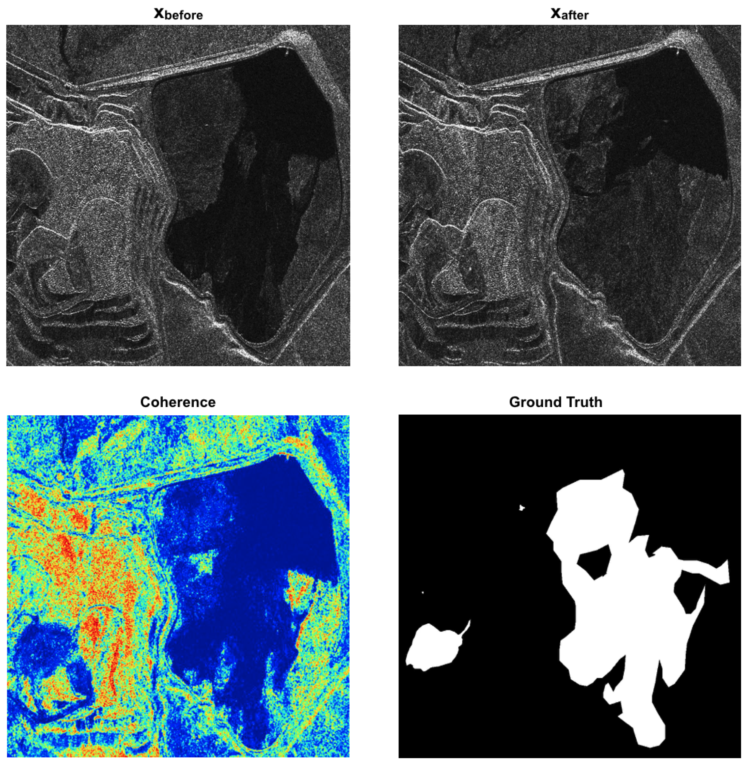Figure 1 shows an example of patches extracted from our SAR change detection training dataset. Coherence plays a crucial role in providing valuable insights into the stability and continuity of the observed surface. It quantifies the degree of similarity between two radar images captured of the same area at different times. By comparing the phase information of the radar waves reflected from the surface, coherence measurements can reveal changes in the scattering characteristics of the terrain. The coherence values obtained from radar images can offer valuable information about the temporal behavior of an observed surface. Higher coherence values indicate a high degree of similarity between radar returns, suggesting little to no changes in the surface properties over time. This typically corresponds to areas with stable features such as buildings, roads, or permanent structures. On the other hand, lower coherence values signify significant changes in the observed area. These changes can arise from various factors such as alterations in the surface morphology, vegetation growth or removal, changes in water bodies, or the presence of moving objects. In such cases, the coherence measurements capture the temporal discrepancies in the radar wave interactions, reflecting the dynamic nature of the surface and highlighting areas that have undergone changes between the acquisition time points. However, it is essential to underline that in our specific task, areas of low coherence do not always indicate a change of interest. Indeed, for example, areas relating to pseudo changes, even though they may have low coherence values, must not be highlighted as a change. By incorporating coherence information into our change detection methodology, as shown in the Section 4, we gained a more comprehensive understanding of the changes occurring in the observed environment, allowing for a more robust and accurate open-pit mine change detection model.

3. Method

Change detection is the process of identifying changes in a scene between two or more co-registered acquisitions. We defined change detection as a binary segmentation task carried out on pair of SAR images of the same area. The goal is to generate a binary map $y\in {\{0,1\}}^{H\times W}$ such that $y(i,j)=1$ when there is a change in location $(i,j)$ and $y(i,j)=0$ when there is not. Our change detection model employs a U-Net [36], a standard encoder–decoder CNN used for semantic segmentation. The small number of training patches available was the primary motivation behind utilizing the U-Net architecture. As previously mentioned, to achieve a well-balanced training dataset with approximately 50% of the patches containing at least one change pixel, we applied a random subsampling technique to discard patches without changes. By reducing the number of negative samples in the training data, we ensured a more stable and effective training procedure, mitigating the impact of the small number of training patches on the model’s performance. This approach allowed us to maximize the utility of the available training data and optimize the change detection capabilities of our model. By utilizing the U-Net architecture, we tried to optimize the performance of our change detection model, despite the challenges posed by the small dimensions of our dataset, and to effectively capture and leverage contextual information while minimizing the risk of overfitting. Despite that, in the Appendix A, we compare three different change detection models taken from the literature. As we will show, the results confirm U-Net’s ability to perform well with few training data. Indeed, the comparison of architectures showed a negative impact on open-pit mine change detection performance due to limited training patches. The scarcity of data restricts the models’ ability to adapt to variations and complexities in the open-pit mine environment, necessitating a large and variegated training dataset to achieve accurate change detection results.

Denoting with $z_{before}\in {\mathbb{C}}^{H\times W}$ and $z_{after}\in {\mathbb{C}}^{H\times W}$ the two SAR complex images, let us define $x_{before}$ and $x_{after}$ as their amplitude and $\rho$ as an estimation [35] of their coherence:

$$\begin{array}{cc}\hfill & x_{before}=\left|\right|z_{before}\left|\right|\in {\mathbb{R}}^{H\times W}\hfill \\ \hfill & x_{after}=\left|\right|z_{after}\left|\right|\in {\mathbb{R}}^{H\times W}\hfill \\ \hfill & \rho =C(z_{before},z_{after})\in {\mathbb{R}}^{H\times W}\hfill \end{array}$$

(1)

The range of the amplitude values of real SAR images can be extremely broad, varying across different target sites and radar sensors. This distribution variability can greatly influence the training of deep learning models and, for this reason, we had to normalize the original SAR amplitudes. In this work, we adopted the same modified z-score, followed by a non linear normalization to the range [0–1] used in [35]. First, for the amplitude image $x_i$, we calculate the median absolute deviation (MAD) value using the following equation:

$$MAD=median\left(\right|x_i-x_{dataset}\left|\right)$$

(2)

Here, $x_{dataset}$ represents the median amplitude computed over the entire dataset. Next, we transform the data into the modified Z-score domain by applying the following equation:

$$x_i^{mz}=\frac{0.6745\times (x_i-x_{dataset})}{MAD}$$

(3)

In this equation, $x_i^{mz}$ represents the pixel-wise modified Z score. The fixed constant 0.6745, derived from [37], approximates the standard deviation. This transformation effectively shifts any potential outliers far from zero. To achieve a standardized input data distribution for network training, we apply the hyperbolic tangent (tanh) function, resulting in the equation:

$$x_i^{norm}=\frac{1}{2}(tanh(\frac{x_i^{mz}}{W})+1)$$

(4)

where $x_i^{norm}$ represents the normalized amplitude values. The variable W = 3 serves as an outlier detection threshold. Any data points with $x_i^{mz}$ scores exceeding W are considered potential outliers and are discarded [37]. Finally, we normalize the obtained data to the interval [0, 1]. Our change detection model takes as input the concatenation of the amplitudes and the coherence employing an early fusion strategy:

$$\begin{array}{cc}\hfill & x=(x_{before},x_{after},\rho )\in {\mathbb{R}}^{H\times W\times 3}\hfill \end{array}$$

(5)

$$\begin{array}{cc}\hfill & \widehat{p}={\mathcal{M}}_{\varphi ,\theta }\left(x\right)={\mathcal{D}}_{\varphi }\left({\mathcal{E}}_{\theta }\left(x\right)\right),\mathrm{where}{\mathcal{M}}_{\varphi ,\theta }={\mathcal{D}}_{\varphi }\circ {\mathcal{E}}_{\theta }\hfill \end{array}$$

(6)

where $D_{\varphi }$ and $E_{\theta }$ represent the encoder and decoder components of the model, and $\varphi$ and $\theta$ their weights. The model produces as output a binary probability map:

$${\mathcal{M}}_{\varphi ,\theta }\left(x\right)\in {[0-1]}^{H\times W\times 3}$$

(7)

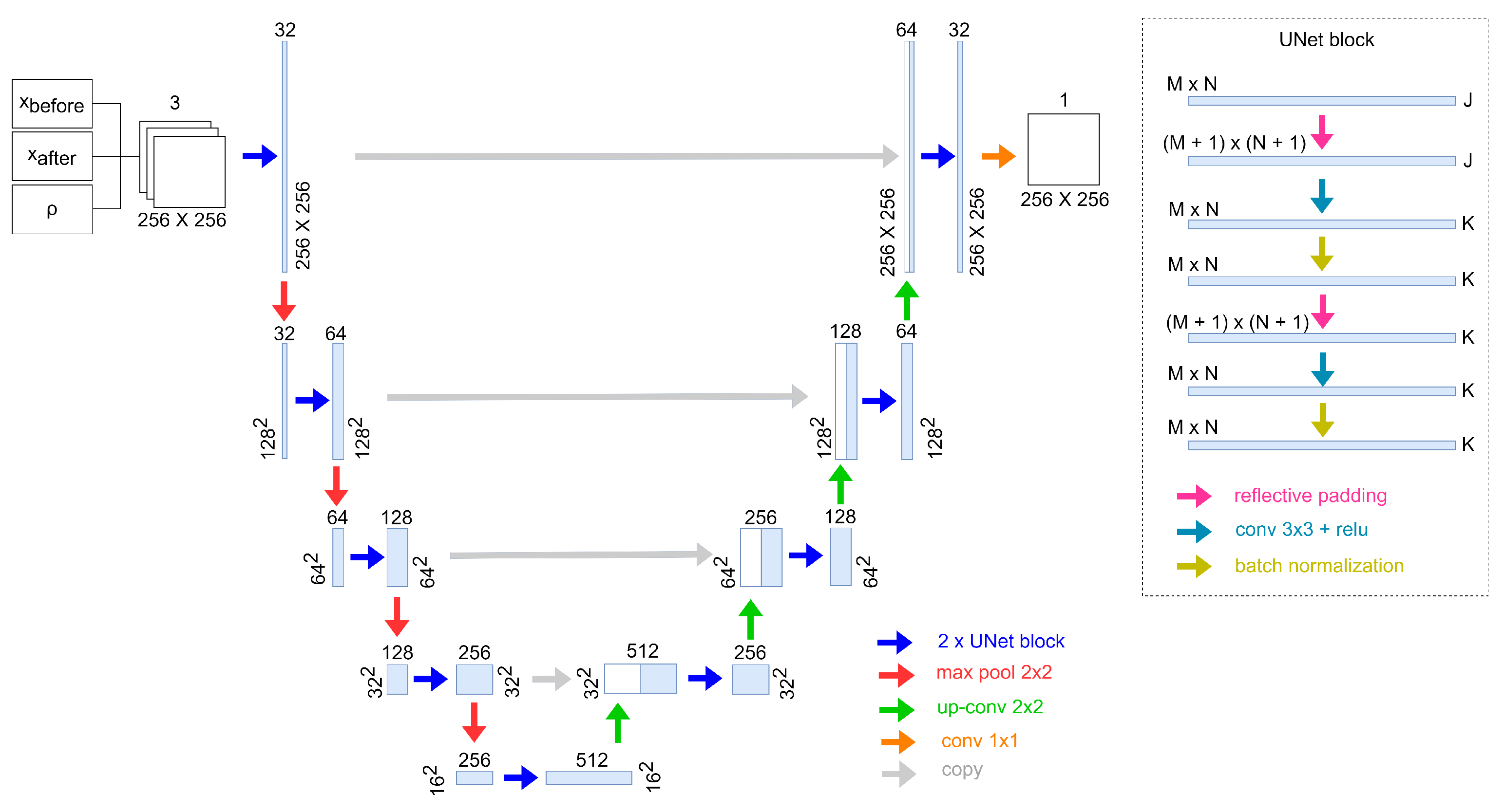
Figure 2 shows the structure used to construct our network. The encoder, which extrapolates useful features compressing the input image, is composed of four convolutional blocks. Each block is structured by stacking a convolutional layer followed by a batch normalization layer and an activation function (ReLU). On the other hand, the encoder path used to retrieve the original image by mapping back the latent representation is composed of another four convolutional blocks structured like the encoder blocks. In order to train our model, we employed binary cross entropy loss:

$$\begin{array}{c}\hfill {\mathcal{L}}_{\varphi ,\theta }(y,x)=-ylog\left({\mathcal{M}}_{\varphi ,\theta }\left(x\right)\right)+(y-1)log(1-{\mathcal{M}}_{\varphi ,\theta }\left(x\right))\end{array}$$

(8)

where y represents the label. Due to the small size of our dataset, during the model training, we encountered several problems related to the training stability and overfitting. To address these problems, we considered multiple data augmentations and included them during the training of the model. In addition to the classic geometric transformations, i.e., vertical/horizontal flip and shear, we introduced custom data augmentations. Input channel swap is an operation used to make the model invariant to the temporal order in which the change occurred. It is computed by simply swapping the order of the $x_{before}$ and $x_{after}$ images in the network input.

Finally, we implemented a custom data augmentation for coherence. In particular, the method consisted of randomly scaling the coherence in areas without change and having a coherence lower than a predefined threshold $\tau$.

$$\begin{array}{c}\hfill {\rho }_{aug}(x,y)=\left\{\begin{array}{cc}\rho (x,y)·u,\hfill & y(x,y)=0\mathrm{and}\rho (x,y)<\tau \hfill \\ \hfill & \mathrm{where}u\sim Uniform[0-1]\hfill \\ \rho (x,y),\hfill & \mathrm{otherwise}\hfill \end{array}\right.\end{array}$$

(9)

In this way, we forced the network not to perform a simple coherence threshold, thus making it robust for areas characterized by low coherence values (e.g., forest, grass) but which do not contain a change of interest. The selection of each data augmentation was carried on empirically by individually selecting it if it improved the validation results with respect to the baseline without augmentations. Appendix B summarizes all the tested data augmentation techniques and their individual improvement in the overall F1-Score.

Pseudo Labeling

To further improve the performance of our model, we also tested a pseudo-labeling pipeline whose patch selection mechanism was extracted from two existing methodologies in the literature [38,39]. Pseudo-labeling techniques use the network’s output as labels for additional training data. This allows the network to use unlabeled data, which can be particularly useful when annotated data are scarce or expensive to obtain. The two categories of pseudo-label techniques are online and offline methods. Online generation creates pseudo-labels iteratively during the training process. On the other hand, offline generation generates pseudo-labels only once during training. The benefit of offline learning is that the pseudo-label does not change with each iteration, and the more iterations we train before the generations, the higher the quality of the pseudo-label. Instead, the online generation approach requires a consistent quality of pseudo-label during the training process. Unfortunately, in the SAR domain, the amplitude distributions acquired in different areas are not always comparable. As a result, introducing pseudo-labels online makes training unstable. We, therefore, opted to generate labels offline and retrain the network from scratch using the expanded training set.

For a binary classification task, let

$$\begin{array}{c}\hfill D=\{(x_i,y_i):i\in (1,\dots ,N)\}\end{array}$$

(10)

be the labeled set with N samples, where $y_i$ is the ground truth of the ith sample and $x_i$ its corresponding feature image, as defined in Equation (5). Let define

$$\begin{array}{c}\hfill U=\{u_i:i\in (1,\dots ,M)\}\end{array}$$

(11)

as an unlabeled set with M samples, where $u_i$ is the feature image of the ith sample. We first train the CNN on the labeled training set D, ${\mathcal{M}}_D$. Once the network is trained on the initial labeled training set D, we then used this to predict the labels for the unlabeled set U. In particular, we use the model trained using D to generate the predictions for the unlabeled set U. We then identify the patches, as in [39], where we are confident in the change or no change classification for at least 90% of pixels within the patch.

$$\begin{array}{c}\hfill \widehat{I}=\left\{i\right|\left(\sum _{\begin{array}{c}w=1,\dots ,W\\ h=1,\dots ,H\end{array}}\mathbb{1}(\left({\mathcal{M}}_D\left(u_i\right)\right)(w,h)>c)\right)>(q·H·W)\forall i\in \{1,\dots ,M\}\}\end{array}$$

(12)

where $c=0.85$ is the confidence threshold, $q=0.9$ is the pixel proportion threshold, $\mathbb{1}$ is the identity matrix, and h and w are the dimensions (height and width) of the image. Finally, we add these predicted labels to the training, selecting a maximum number of them to be at most equal to the number of the original training set, as

$$\begin{array}{cc}\hfill & I\subseteq \widehat{I}s.t.\left|I\right|\le N\hfill \\ \hfill & \widehat{D}=D\cup \left\{(u_i,\mathbb{1}({\mathcal{M}}_D\left(u_i\right)>0.5))\right|i\in I\}\hfill \end{array}$$

(13)

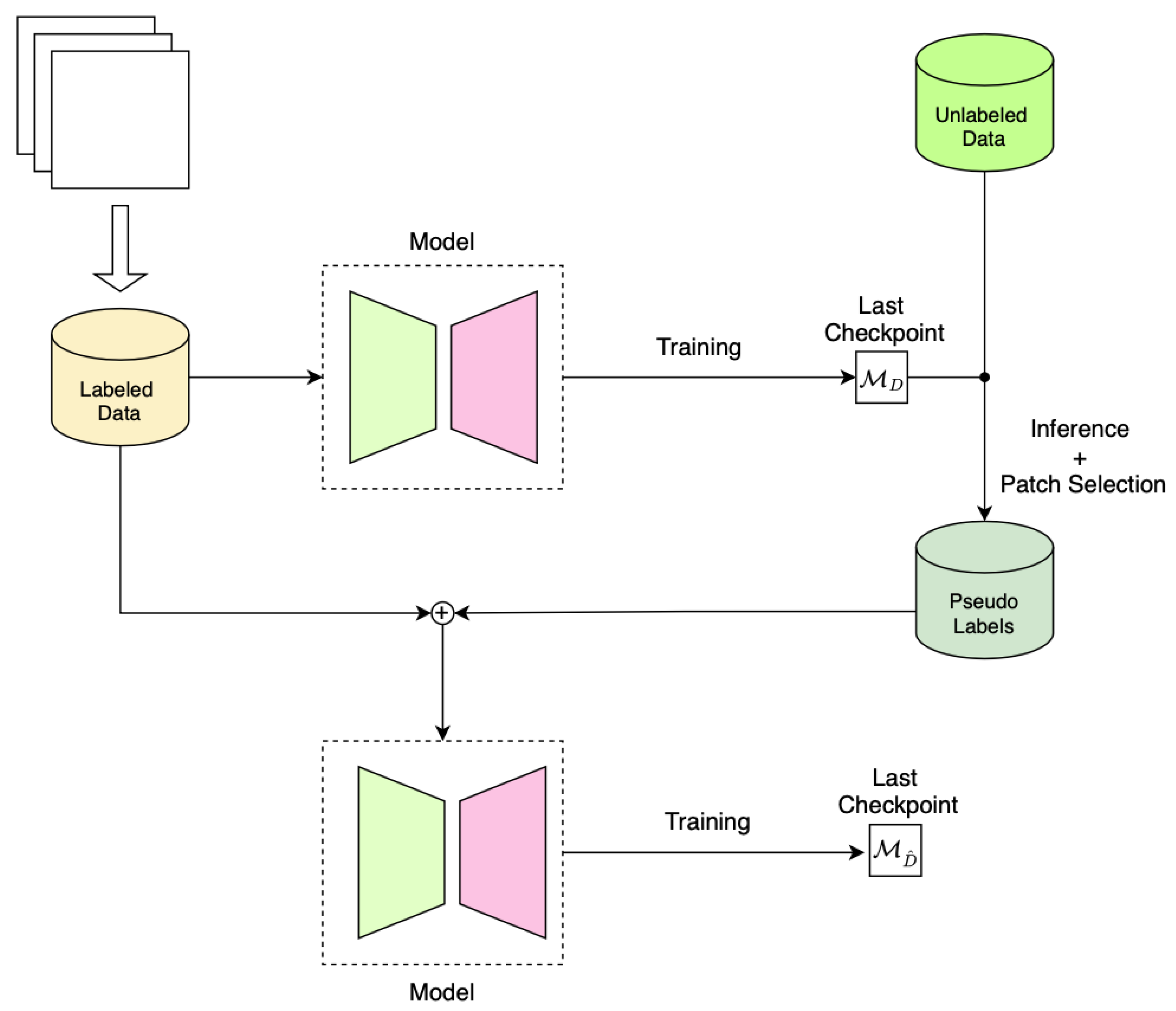
We retrain the network on this new expanded set, using the same loss function as before, Equation (8). Algorithm 1 illustrates the pseudo-code, and Figure 3 shows a schematic view of our pseudo-labeling. In the experiments presented in the next section, we show that the semi-supervised strategy improved the classification performance.

Algorithm 1 Pseudo-labeling pseudo-code

Input: Labeled set $D=\{(x_i,y_i):i\in \{1,\dots ,N\}\}$, unlabeled set $U=\{u_i:i\in \{1,\dots ,M\}\}$, confidence threshold c, pixel proportion thresholds q  1: Train a model on D for K epochs and save the model ${\mathcal{M}}_D$    2: Generate the predictions on the unlabeled set U identifying the patches with high-confidence predictions: $$\begin{array}{c}\hfill \widehat{I}=\left\{i\right|\left(\sum _{\begin{array}{c}w=1,\dots ,W\\ h=1,\dots ,H\end{array}}\mathbb{1}(\left({\mathcal{M}}_D\left(u_i\right)\right)(w,h)>c)\right)>(q·H·W)\forall i\in \{1,\dots ,M\}\}\end{array}$$  3: Select pseudo-labels number at most equal to N $$\begin{array}{c}\hfill I\subseteq \widehat{I}s.t.\left|I\right|\le N\end{array}$$  4: Add pseudo-labels into D: $$\begin{array}{c}\hfill \widehat{D}=D\cup \left\{(u_i,\mathbb{1}({\mathcal{M}}_D\left(u_i\right)>0.5))\right|i\in I\}\end{array}$$  5: Retrain the model from scratch using $\widehat{D}$ as training set

4. Results

All the experiments were performed using PyTorch with an NVIDIA Tesla T4.

Table 4. Training optimizer parameters used for validation.

Parameters Configuration
	${\mathit{A}}^{\mathit{Train}}-{\mathit{B}}^{\mathit{Val}}$	${\mathit{B}}^{\mathit{Train}}-{\mathit{A}}^{\mathit{Val}}$
Optimizer	AdamW [40]	AdamW [40]
Base learning rate	1 × 10${}^{-3}$	1 × 10${}^{-3}$
Weight decay	0.01	0.01
Amsgrad	False	False
Momentum	${\beta }_1,{\beta }_2$ = 0.9, 0.999	${\beta }_1,{\beta }_2$ = 0.9, 0.999
Batch size	64	64
Training epochs	300	400
Scheduler step	270	370
Scheduler value	0.1	0.1
Precision	Mixed precision (16 bit)	Mixed precision (16 bit)

summarizes the training parameters used for both two-fold cross-validation baseline experiments.

We evaluated the performance of our proposed method using $F1$ score with respect to the change class as

$$\begin{array}{cc}\hfill & F1=2·\frac{Precision·Recall}{Precision+Recall}\hfill \end{array}$$

where

$$\begin{array}{cc}\hfill & Precision=\frac{TP}{TP+FP}\hfill \\ \hfill & Recall=\frac{TP}{TP+FN}\hfill \\ \hfill \end{array}$$

$TP$, $TN$, $FP$, and $FN$ are computed for the change class, and represent the true positives, true negatives, false positives, and false negatives, respectively. To retrieve the change mask we applied a 0.5 threshold to the output mask.

4.1. Results on the Validation Sites

In the initial baseline experiments, we employed a U-Net model that solely utilized the concatenated amplitude information from the two acquisitions as input. However, as indicated in the first row of

Table 5. Validation results. We the report mean ± std of three runs.

F1-Score
Configuration	${\mathit{A}}^{\mathit{Train}}-{\mathit{B}}^{\mathit{Val}}$	${\mathit{B}}^{\mathit{Train}}-{\mathit{A}}^{\mathit{Val}}$
Pseudo-Label Set	$\mathit{B}$	$\mathit{A}$
Baseline	$0.4515\pm 0.0288$	$0.5645\pm 0.0270$
+ Coherence	$0.6825\pm 0.0163$	$0.6375\pm 0.0165$
+ Augmentations	$0.7064\pm 0.0207$	$0.7730\pm 0.0096$
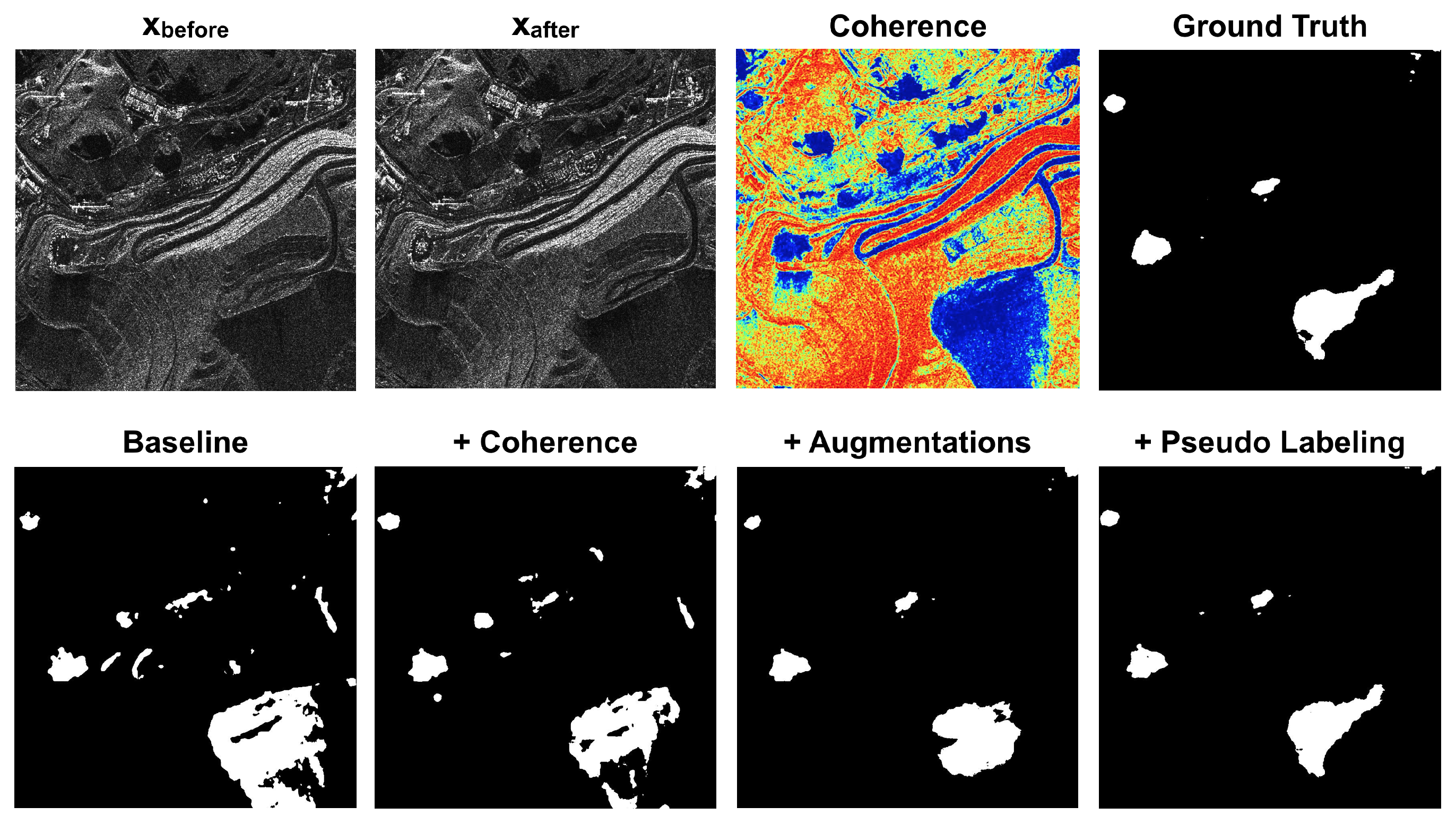
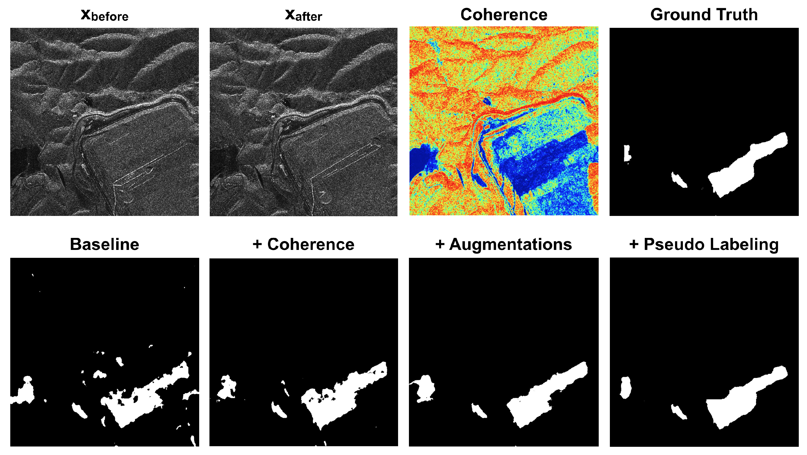
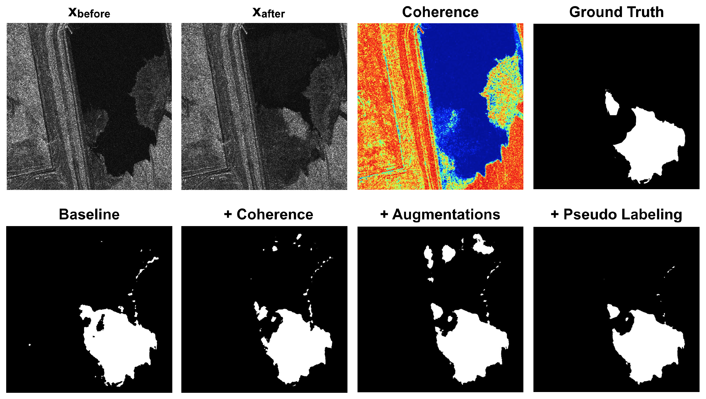
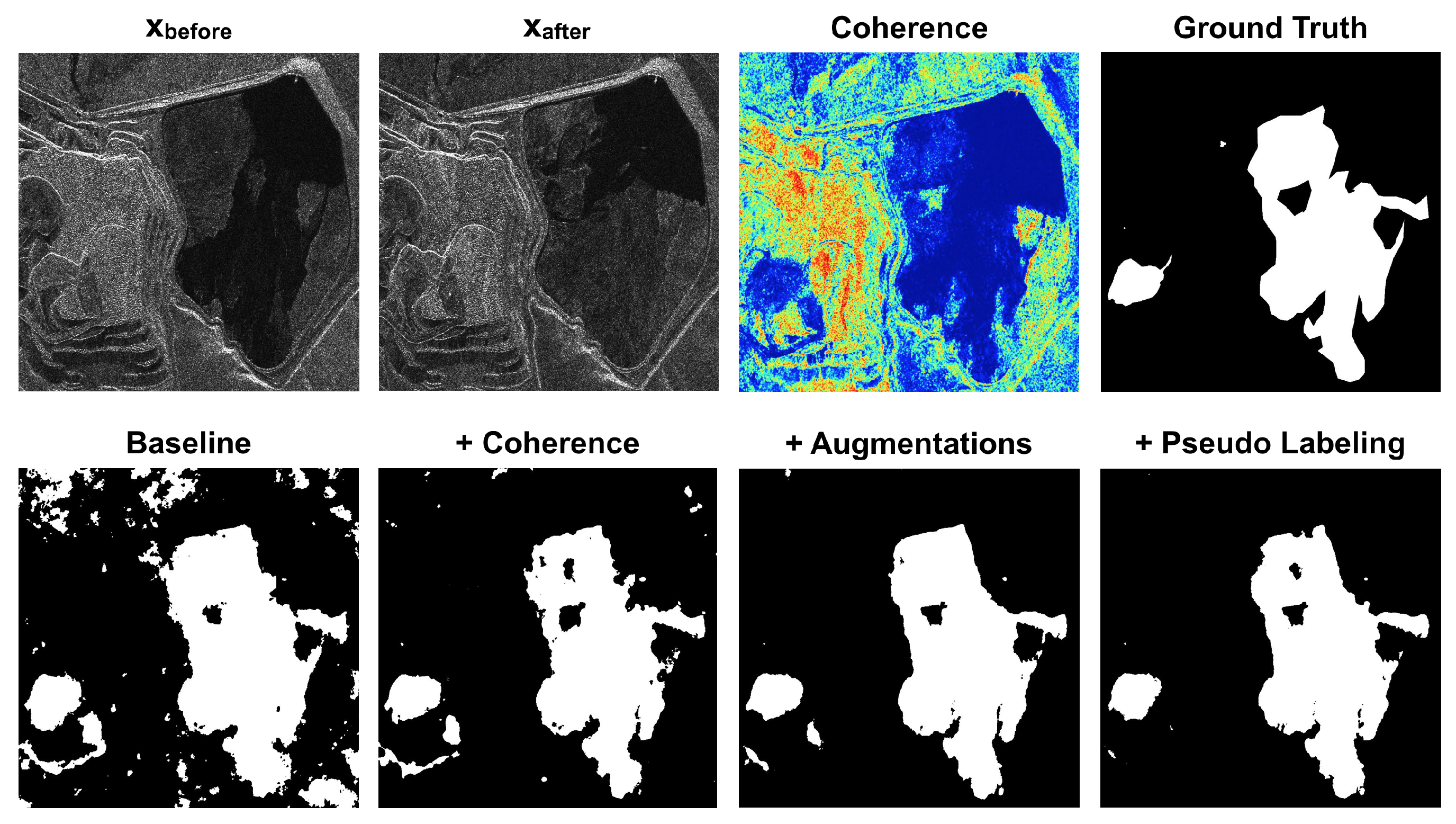
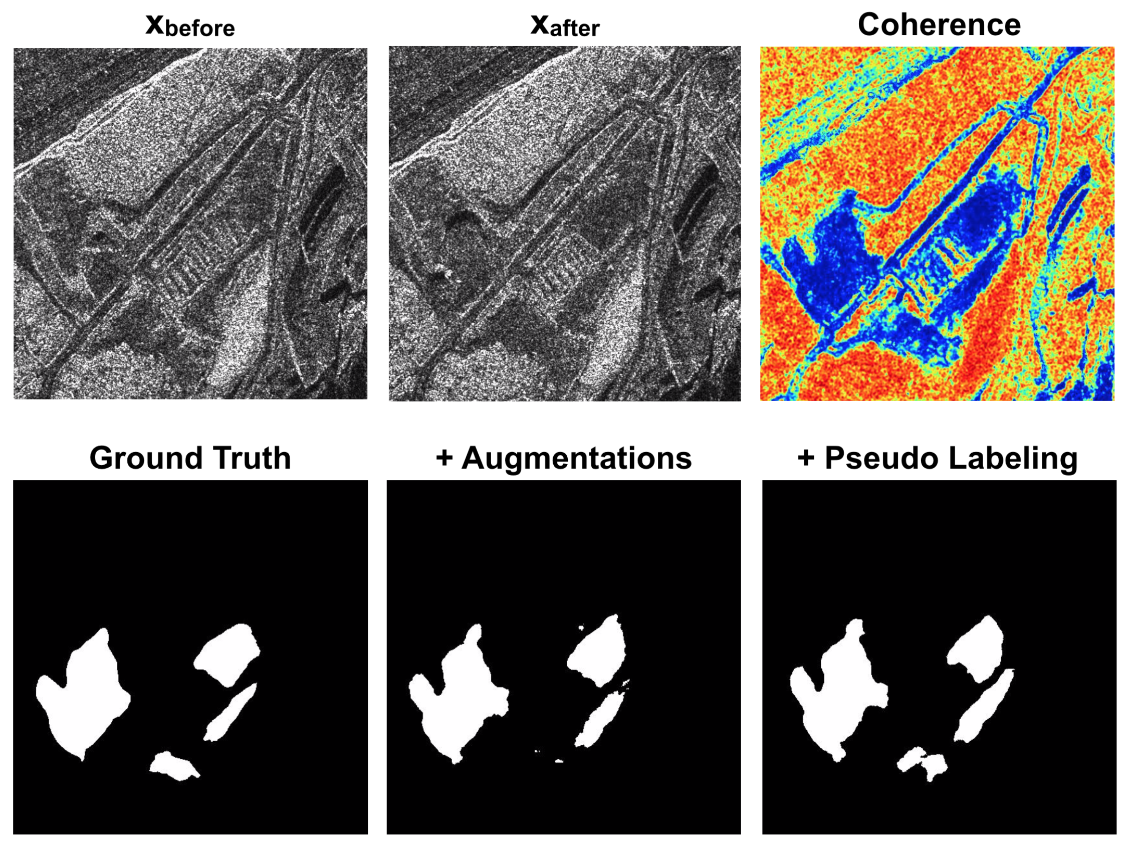
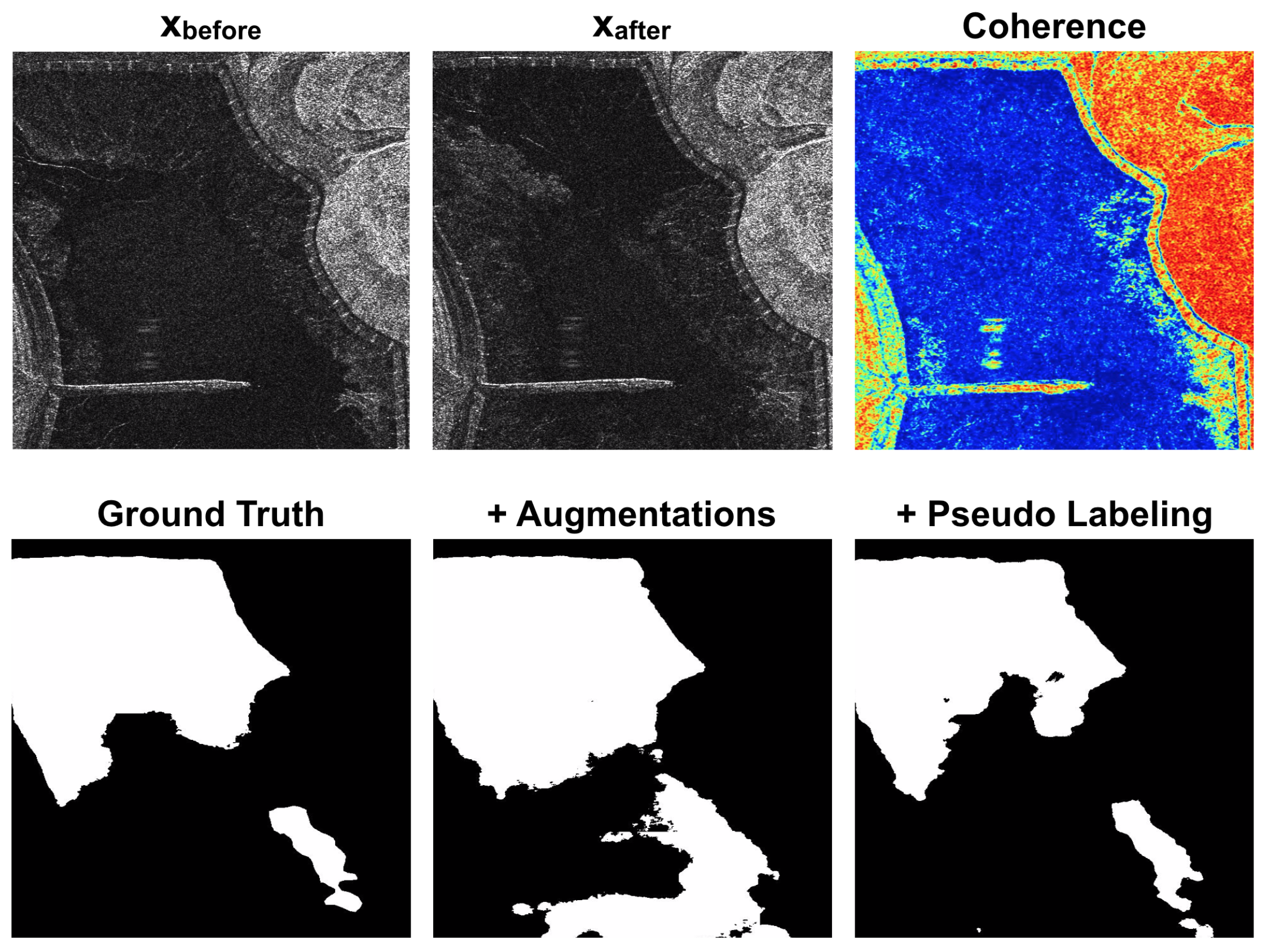
+ Pseudo Labeling	$\mathbf{0.7459}\pm 0.0111$	$\mathbf{0.7938}\pm 0.0206$

, the results demonstrated low F1-score values. It became evident that the model struggled to classify the changes accurately. Indeed, as shown in Figure 4, Figure 5, Figure 6 and Figure 7, the baseline model introduced false positives in areas where we did not have an effective change, despite the low coherence values associated with them. Indeed, areas characterized by low coherence values do not necessarily contain a change of interest. It is also possible to highlight that the model trained with site B, despite a low number of training patches, i.e., 188, generalized better on the validation set with respect to the other configuration (Site A used for training). This behavior is caused by the fact that mining area land use types are highly complex and heterogeneous. Mining sites frequently have different amplitude distributions, due to the diverse land cover types within a single scene. This heterogeneity, which complicates the detection and distinction of changes within open-pit mines, demonstrates the need for training a model for this specific task.

We conducted subsequent experiments to investigate the potential benefits of incorporating the coherence layer as an additional feature. Including coherence information in the network yielded performance improvements, as illustrated in Table 5. The coherence proved to be particularly valuable in both the two-fold cross-validation setups. This outcome was significant, considering that Site A and Site B exhibited distinct amplitude distributions among their respective patches. Consequently, the coherence played a crucial role in bridging the gap between these diverse amplitude distributions. In addition, as shown in Figure 4, Figure 5, Figure 6 and Figure 7, the coherence helped the network to reduce false positive and better delineate the edges of the change areas. Building upon these findings, the subsequent experiments were designed to utilize the following fixed inputs: the amplitude of both images, and the coherence between them.

The limited size of our dataset presented challenges in terms of model training instability and the potential for overfitting. To mitigate these issues, we implemented various data augmentation techniques during the training process. By introducing these augmentations, we aimed to enhance the robustness and generalization capabilities of the model. The results of the trained model, incorporating all the described data augmentation techniques, are presented in Table 5. As shown, the introduction of data augmentations yielded improved F1-scores in both two-fold cross-validation setups. This outcome highlights the effectiveness of the augmentation strategies in enhancing the performance of the model. By augmenting the dataset, we were able to increase the diversity and variability of the training samples, enabling the model to learn more effectively and achieve better overall results. Also in this case, Figure 4, Figure 5, Figure 6 and Figure 7 show the improvement in the predictions.

To further enhance the results achieved using data augmentation techniques, we implemented a pseudo-labeling pipeline that leveraged the network’s output as labels for additional training data. The two-fold cross-validation setups were crucial in evaluating the consistency and effectiveness of this proposed methodology. We identified the 200th epoch as the optimal candidate for generating pseudo-labels for all the experiments conducted. Subsequently, we retrained the network from scratch, employing 100 epochs for the first configuration ($A^{Train}-B^{Val}$) and 200 epochs for the second configuration (Site $B^{Train}-A^{Val}$). 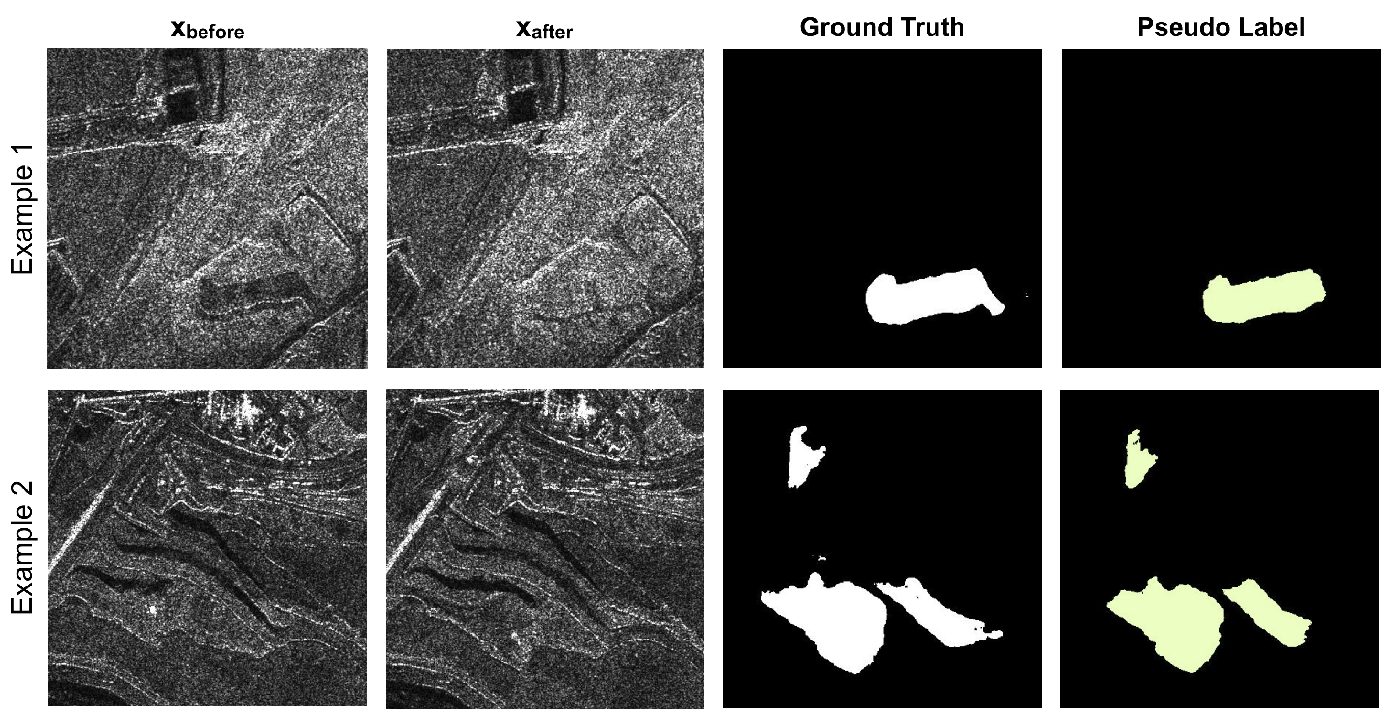It is important to note that we selected the validation sets as the unlabeled sets in both cases. The decision to use the validation dataset as an unlabeled dataset was mainly due to two reasons. First, we wanted to demonstrate how inserting images, which we validated in training, actually benefited the validation performance. Indeed, as previously explained, different areas can have very different amplitude distributions in SAR images. Therefore, the introduction of new different patches compared to the training patches extracted for a single site helped the model to increase performance. At the same time, the other motivation was related to being able to check the pseudo-labels with respect to the real ground truths. As depicted in Figure 8, the quality of the pseudo-labels generated by the final checkpoint exhibited high accuracy without introducing misclassification points associated with pseudo-change areas. This pseudo-label accuracy subsequently led to a notable performance enhancement when incorporated into the dataset for model retraining. Including the pseudo-labeled data effectively contributed to further refining the model’s ability to detect changes, resulting in an improved overall performance, as shown in Table 5. This meant that the approach also allowed for the flexibility of retraining the model using a new mining site as an unlabeled dataset, whenever predictions were required for that particular site. To further assess the model’s performance, we visually examined its outputs on selected examples extracted from both the validation sets. As depicted in Figure 4, Figure 5, Figure 6 and Figure 7, the retrained model exhibited accurate detection of changes within the mining sites. This included the identification of large-scale changes, such as the expansion of the mining pit, as well as small-scale changes. Additionally, the model effectively mitigated false positives associated with pseudo changes, correctly identifying stable areas as unchanged.

As we will demonstrate in the next section, the introduction of pseudo-labels during the retraining phase enhanced the model’s generalization capacity, even when applied to a third site (Site C) that was previously unknown to the model. By leveraging the information contained within the pseudo-labels and incorporating them into the training process, the model became more adept at detecting changes in unseen areas. This capability showcases the robustness and adaptability of our approach, as the model successfully extended its change detection capabilities to a new and unfamiliar site.

4.2. Results on the Test Site

We selected Site C as the test site to evaluate our change detection model’s performance. Site C remained entirely unseen by the model during the training and validation stages, thus providing a proper assessment of its generalization capabilities. This test site possesses distinct characteristics compared to Site A and Site B, introducing new challenges that the model had to effectively address to be considered a reliable change detection tool. To evaluate the model’s performance on Site C, we employed both two-fold cross-validation configurations. In particular, we conducted a comparative analysis between models trained with and without the inclusion of pseudo-labeling, utilizing the data augmentation strategies in both cases. The results of the model’s performance on our test site are presented in

Table 6. Test results. We report the mean ± std over three runs.

F1-Score
	${\mathit{A}}^{\mathit{Train}}-{\mathit{B}}^{\mathit{Val}}$	${\mathit{B}}^{\mathit{Train}}-{\mathit{A}}^{\mathit{Val}}$
Pseudo-Label Set	$\mathit{B}$	$\mathit{A}$
+ Augmentations	$0.7549\pm 0.0086$	$0.7652\pm 0.0077$
+ Pseudo Labeling	$\mathbf{0.7908}\pm 0.0118$	$\mathbf{0.7742}\pm 0.0106$

. This evaluation allowed us to demonstrate the model’s ability to detect changes accurately and reliably in a previously unseen environment, providing valuable insights into its real-world applicability and generalization capabilities.

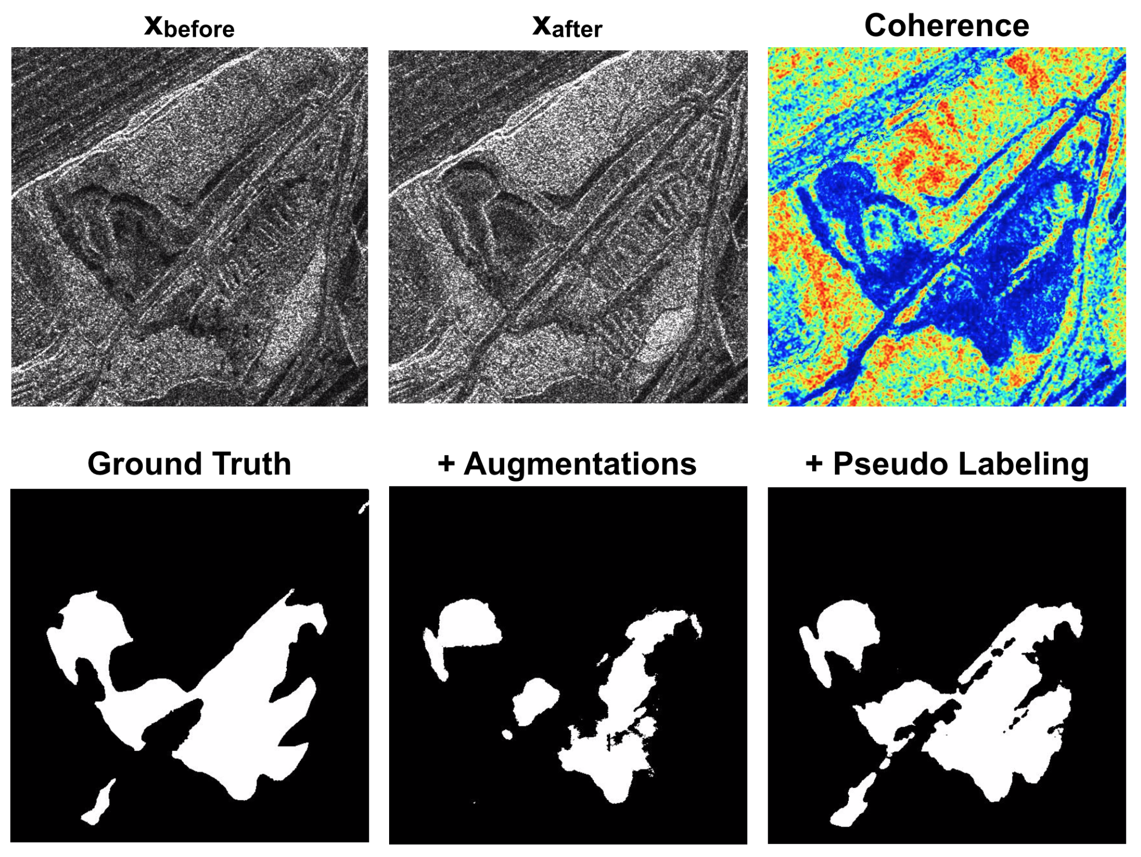
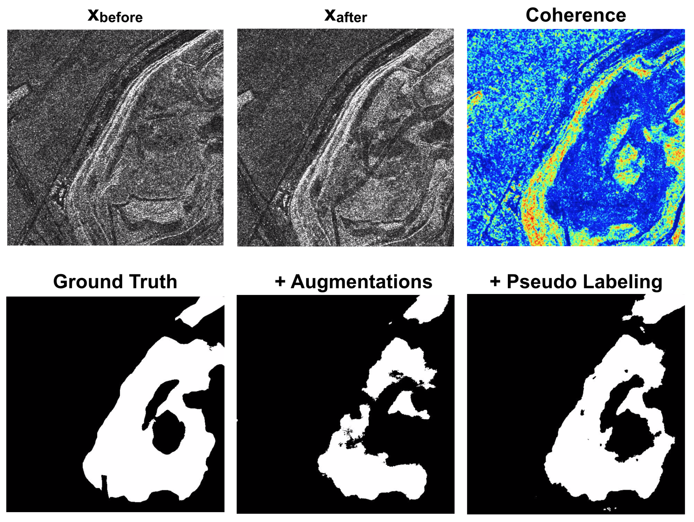
The effectiveness of our proposed deep learning methodology for change detection in the mining sector using SAR images is demonstrated through the visual examples depicted in Figure 9, Figure 10, Figure 11 and Figure 12.

The retrained model showcased its capability to accurately detect changes of various scales, encompassing both large-scale transformations and slight alterations within the mining sites. These visual examples prove the model’s ability to accurately discern changes. It identified and highlighted significant changes, suppressing false positives and ensuring that stable areas were appropriately classified as unchanged. In summary, our results demonstrate the efficacy of our proposed deep learning methodology for change detection in the mining sector using SAR images. The model consistently achieved high F1-score values, indicating its robust performance in accurately identifying changes within the mining sites. These findings emphasize the potential of deep learning approaches to deliver reliable and precise change detection outcomes in the mining sector, leveraging the power of SAR data for enhanced monitoring and decision-making processes.

5. Discussion

As already highlighted in [10], the need for a specialized model trained on open-pit mines arises from the complex nature of this domain. Unlike many traditional change detection tasks, open-pit mines present unique challenges. The coexistence of diverse land cover types, coupled with various types of changes within the mining environment, makes this a particularly intricate task. Furthermore, SAR images can be challenging to interpret due to their complex interactions with the ground. Indeed, the backscatter signal may vary significantly based on surface roughness, incidence angle, and temporal differences [41]. To address these challenges, our study focused on developing a deep learning model specifically tailored to open-pit mine change detection. We acknowledged the limitations of traditional signal processing methods [30] and, by doing so, aimed to achieve more effective and accurate change detection in this sector. The low F1-score values in Table 5, obtained when employing only the amplitude information, demonstrate that the model could not generalize on different land cover distributions and only classified areas linked to actual changes related to mining operations. Thus, SAR amplitude data alone may not capture specific, subtle changes effectively or distinguish slight variations. The pivotal roles of data augmentations and the coherence layer as indispensable elements were confirmed by the significant improvements in the F1-score values. As shown in Table 5, coherence proved to be additional information fundamental for eliminating false positives related to pseudo changes and for addressing the lack of data, which does not allow the model to generalize from different amplitude distributions. It is essential to highlight that our method is the first in the literature to employ coherence with amplitude in a change detection task, underscoring the potential of InSAR data when integrated effectively into deep learning frameworks. On the other hand, as shown in Table 5, Table 6 and

Table A2. Data augmentations that were individually evaluated.

Data Augmentation	F1-Score
Baseline	-
Veritical Flip	+3.8%
Horizontal Flip	+6.6%
ShearY $[-{10}^{\circ },+{10}^{\circ }]$	+5.1%
Swap	+4.3%
Coherence Scaling [$\tau$ = 0.10]	+2.5%

, the data augmentation techniques employed were found to have a significant positive impact on the performance of our change detection model, helping the model to mitigate overfitting and improve robustness; despite being SAR acquisition side-look, the image physical structures were not always preserved. Finally, the F1-score values in Table 5 and Table 6 illustrate how, when dealing with a limited number of labels, the integration of a pseudo-labeling pipeline could enhance he model accuracy, without compromising its performance by introducing misclassified points associated with pseudo changes. The comparison results in Appendix A highlight the limitations of our work, reinforcing the importance of having a large and diverse training dataset, particularly for complex tasks such as open-pit mine change detection. These findings emphasize the need for further research, to concentrate on strategies for acquiring and augmenting data. By addressing the limitations imposed by the scarcity of training data, we can enhance the performance of deep learning architectures in this domain. Future works will focus on expanding the dataset to incorporate a broader range of diverse mining sites and investigating the applicability of different deep learning architectures for change detection in open-pit mines. Expanding the dataset will allow the inclusion of additional mining sites with distinct characteristics and variations in land use types. This diversity will enable our models to learn and generalize across various scenarios, improving their adaptability and accuracy in change detection tasks. In addition, expanding the dataset will also allow exploring alternative deep-learning architectures that hold potential for advancing the field of open-pit mine change detection. An example could be employing a recurrent model to manage multiple images spanning an extended time period, such as considering a sequence of three or more images. This expanded temporal context could allow a deeper analysis of the progressive changes occurring between multiple time points. Consequently, the model could become more adept at discerning nuanced variations and complex transformations, particularly in regions undergoing gradual or subtle alterations. Through these future perspectives, we aim to enhance the capabilities of our deep learning model in open-pit mine change detection, paving the way for improved monitoring and environmental management practices in the mining industry.

6. Conclusions

In this paper, we proposed a deep learning methodology for change detection in the mining sector using SAR images. The proposed method is based on a CNN architecture, which was trained on a dataset of SAR images of mining sites. SAR data for change detection have several advantages. Indeed, the images can be acquired regardless of weather or lighting conditions, providing information about the earth’s surface. Additionally, they can be used to monitor changes in large areas with high resolution and accuracy, making them an attractive option for monitoring mining operations. Unfortunately, there are no public SAR change detection datasets for the case of open-pit mines. For this reason, despite the high human cost, we created a new dataset annotated by experts in the field. To evaluate the effectiveness of our approach, we conducted experiments on three different mining sites: Site A, Site B, and Site C. These sites were chosen as they represent the types of mining operations commonly found and have different characteristics, providing a comprehensive evaluation of the model’s performance. The visual results of the experiments, together with the F1 Score values obtained, demonstrate that the proposed model could effectively identify changes. The use of coherence information, data augmentation techniques, and a pseudo-labeling algorithm significantly improved the model’s performance. To further evaluate the model’s generalization capabilities, we tested it on Site C, which was completely unseen by the model during training and validation. Our results demonstrate the potential of deep learning approaches for change detection in the mining sector using SAR data. The proposed methodology can provide reliable and accurate results, which can be used to support decision-making in the mining industry, monitor the evolution of mining operations, detect illegal mining activities, or monitor the impact of mining on the environment.