Modeling Uncertainty of GEDI Clear-Sky Terrain Height Retrievals Using a Mixture Density Network

Abstract

Early spaceborne laser altimetry mission development starts in pre-phase A design, where diverse ideas are evaluated against mission science requirements. A key challenge is predicting realistic instrument performance through forward modeling at an arbitrary spatial scale. Analytical evaluations compromise accuracy for speed, while radiative transfer modeling is not applicable at the global scale due to computational expense. Instead of predicting the arbitrary properties of a lidar measurement, we develop a baseline theory to predict only the distribution of uncertainty, specifically for the terrain elevation retrieval based on terrain slope and fractional canopy cover features through a deep neural network Gaussian mixture model, also known as a mixture density network (MDN). Training data were created from differencing geocorrected Global Ecosystem Dynamics Investigation (GEDI) L2B elevation measurements with 32 independent reference lidar datasets in the contiguous U.S. from the National Ecological Observatory Network. We trained the MDN and selected hyperparameters based on the regional distribution predictive capability. On average, the relative error of the equivalent standard deviation of the predicted regional distributions was 15.9%, with some anomalies in accuracy due to generalization and insufficient feature diversity and correlation. As an application, we predict the percent of elevation residuals of a GEDI-like lidar within a given mission threshold from 60°S to 78.25°N, which correlates to a qualitative understanding of prediction accuracy and instrument performance.

1. Introduction

In the lifecycle of space-based mission design, the starting point is pre-phase A, where a broad spectrum of ideas can be explored and evaluated. Level 1 mission requirements drive a myriad of pre-phase A mission development decisions related to orbit design and instrument selection for single or multiple satellites. All three criteria are intertwined, with competing costs and “values” with respect to mission science requirements. Predicting instrument performance with respect to realistic environmental conditions can be difficult, and typically, realism is sacrificed for computational feasibility, leading to sub-optimal design. As an example, missions looking to measure global elevation need to explore all the scenarios of the surface structure, composition, reflectivity, and attenuation as components that impact the ability of the sensor to adequately capture the measurement. Often, laser altimetry (lidar), an active sensing technology, is selected to observe the Earth’s surface in three dimensions and requires a comprehensive analysis of the energy link budget during pre-phase A studies. The utility of measuring height at the global scale supports the Decadal Survey (DS) observational needs across a diverse number of scientific communities [1]. Although space-based lidar is a relatively new remote sensing technology for Earth observation compared to other sensing types, it has been proven to support measured needs associated with surface topography, vegetation structure, cryospheric processes, and shallow water bathymetry, with high vertical accuracy [2]. Unlike imaging systems or synthetic aperture radar (SAR), lidar can penetrate dense canopies, revealing details in the underlying topography and vertical structure of the vegetation.

Having knowledge of laser altimetry’s capabilities from previous planetary missions using the technology, NASA launched the first Earth observing satellite laser altimeter in 2003. This mission, ICESat (Ice, Cloud, Land Elevation Satellite), was primarily focused on quantifying changes in our polar ice sheets and sea ice, as hot spots of climate impact on sea-level rise and the radiative balance between the ocean/land and atmosphere [3]. However, the instrument operated globally, so it was able to capture measurements of vegetation, oceans, atmosphere, and mid-latitude topography. ICESat was operational until decommissioning in 2009 after serving a wide range of scientists using altimetry to study Earth systems. Following the success of ICESat, ICESat-2—operational in 2018—continued the focus on the cryosphere, including measuring changes in sea ice freeboard and ice sheet elevation in Greenland and Antarctica [4]. The combined data products from the ICESat and ICESat-2 missions have made significant contributions to a ~20-year timeseries of cryospheric response to changes in the atmosphere and ocean conditions [4].

Using the success of ICESat lidar technology, but designed for mid-latitude vegetation, NASA developed the Global Ecosystem Dynamics Investigation (GEDI). GEDI science goals are focused on measuring ecosystem structure, namely canopy heights, to derive above-ground biomass and inform global carbon stocks [5]. Through full-waveform lidar technology, the GEDI provides vertical profiles of forest structure ideal for tropical and temperate regions. The GEDI height distributions initialize and constrain [5,6] the predictive outputs of the Ecosystem Demography model [7], directly supporting carbon flux estimation and its role in providing a greater understanding of climate change. All three space-based lidar mission products have been fused with Landsat [8], TanDEM-X [6], and other mission products [5,9] to enhance and/or calibrate optical and radar-based measurements.

Clearly, there is great utility in maximizing the output of a novel lidar-based mission concept. Striking a balance between realism and analytic estimates of lidar performance, we introduce a statistical approach to assess whether lidar instrument performance meets mission requirements. We narrowly focus our study on modeling GEDI lidar-measured elevation uncertainty based on terrain slope and canopy fractional cover for surface topography and vegetation applications, to provide a baseline work for future studies to adapt.

Lidar modeling techniques range from macroscopic approximations of performance as it pertains to measurement objectives [10,11,12,13], to highly detailed simulations of the absorption of light through the atmosphere and its reflectance off of vegetation, terrain, or urban landscapes [14,15,16]. Analytic estimates of architecture performance can be derived from simplifications of the lidar equation, assuming mean surface reflectance and atmospheric transmittance [10,13]. For simple reflectance geometries, explicit formulas for the change in waveform are tractable [17]. When applied to many microfacets, the aggregation of differential changes in the transmitted waveform results in realistic return waveforms [17,18]. At the other end of the spectrum, 3D radiative transfer (RT) models, such as the Discrete Anisotropic Radiative Transfer (DART) model [16], account for the absorption, emission, and scattering of radiation, using external or RT-derived tabular data on the physical characteristics of a scene, through a combination of Monte-Carlo and ray-tracing methods. While comprehensive, RT models are computationally demanding and may not be applicable in preliminary mission design at the global scale.

Between these two extremes, the GEDI Simulator is a data-driven approach to simulate return waveforms, purpose-built for the calibration and validation of GEDI data products [19,20]. Instead of simulating radiance interactions, the GEDI Simulator aggregates high-resolution airborne lidar survey (ALS) point clouds to create waveforms, a technique originally conceptualized by Blair and Hofton [21]. A stark advantage of the GEDI Simulator is that it does not require optical properties of terrain and vegetation structure, as is necessary with RT models. However, its simulation domain is limited to the extent of the available reference lidar.

Aside from classification, machine-learning (ML) methods are commonly applied in an inverse problem setting to estimate a physical property from measurements [22], such as above-ground biomass, canopy height, or canopy cover. For example, the GEDI science team developed a convolutional neural network to predict canopy heights more accurately from GEDI waveforms [23]. Contrary to traditional lidar applications of ML, we seek to model the elevation return quality based off of the physical properties of the Earth’s surface; therefore, our technique loosely falls under forward modeling, for modeling the uncertainty of GEDI terrain elevation measurements.

We model the footprint-level elevation residual distribution (ERD) as a Gaussian mixture model (GMM), predicted through a Mixture Density Network (MDN) [24,25], which is a deep neural network (DNN) with special activation functions at the output layer that produces mixing coefficients, means, and standard deviations for each component of the GMM. With a GMM, we can fit the near Cauchy-like ERD while maintaining generality for more mountainous or vegetated regions that could have less linear elevation residual variance than flatter, barren regions. Our key innovation is to fit at the footprint scale, but attempt to predict elevation residuals over entire areas, estimating a so-called “regional elevation residual distribution” or RERD. We therefore train the ERD on a traditional 80/20 split but choose hyperparameters based on RERD predictions to better isolate generality from local to global scales. In Section 2, we discuss the reference lidar and GEDI measurement data used to train the MDN, thoroughly discuss the development of RERD prediction, and end with a summary of the methodology. Then, in Section 3, we show model validation and accuracy using a five-fold cross-validation. Finally, we conclude with a discussion in Section 4.

2. Materials and Methods

2.1. Overview

We seek to train a model based on terrain slope and canopy cover input features to predict the geocorrected elevation residual in the version 2 L2B GEDI elevation measurements at non-polar latitudes as a means to explore the performance of the GEDI instrument. Our baseline model choice is a neural network-based Gaussian mixture model (GMM), known as a Mixture Density Network (MDN) [24,25]. With a properly trained model, we can predict what the elevation measurement quality of a spaceborne, GEDI-like lidar will be, given any location on land, where trained features are applicable. The predicted ERDs are fundamentally meter-scale, but such a resolution is computationally prohibitive and overly precise for a global, conceptual mission design. We therefore downsample the predictions to the km-scale, outputting the distribution of elevation residuals over large spatial regions (RERDs), given the terrain and vegetation structure of those regions. We develop training data by differencing the measured GEDI elevation against airborne lidar surveys (ALS), then correlate slope and cover features with elevation residuals to train the model. Through a statistical aggregation, we predict how GEDI elevation residuals are distributed throughout entire spatial regions of the Earth’s land surface. In this section, we describe the reference lidar, GEDI L2B elevations, modeling theory, and implementation details.

2.2. Reference Lidar

Airborne lidar surveys (ALS) typically produce centimeter-level accurate point-clouds [26], containing a high-resolution 3D structure of the terrain and vegetation in a km-scale region. If they are temporally consistent, GEDI waveforms can be directly compared to reference lidar to validate derived datasets such as canopy height, terrain elevation, or the entire waveform [19,27]. For terrain-only applications, the lowest mode of the GEDI waveform elevation retrieval can be compared to high-resolution raster digital terrain models (DTMs) of ground-classified reference lidar [28] to determine the fidelity of the spaceborne measurements.

In recent years, Refs. [27,29,30] have validated GEDI elevation and canopy height accuracy against the National Ecological Observatory Network (NEON) discrete return point clouds. NEON has an open-source easy-to-use interface to query reference lidar, with collection dates from 2013 to 2023, with 59 collection sites in the United States, including regions in Hawaii, Alaska, and Puerto Rico [31]. The NEON airborne observation platform deploys an Optech Gemini lidar for the discrete lidar product, maintaining measurement quality for each region of interest (ROI) to <5–15 cm horizontal accuracy (1$\sigma$) and <5–35 cm vertical accuracy (1$\sigma$) [27]. All NEON reference lidar tiles are referenced to the WGS84 ITRF2000 ellipsoid horizontal datum, with the NAVD88 vertical datum using GEOID12A [32].

The temporal differences between the measured and reference lidar can lead to additional uncertainty in comparisons [27]. GEDI launched in late 2018 on a 2-year mission, starting in April 2019 after on-orbit checkout [5]. Because a third of 2019 does not have GEDI data, and because 2020 does not have a sufficient number of NEON reference tiles, we chose the year 2021 to optimize both the amount of temporally consistent GEDI data and abundance of NEON reference data, while simplifying the comparisons to a single year of reference lidar. To compare interannual trends in ecology, NEON ALS measurements are taken during the spring and summer when vegetation is at maximum greenness [32]. In this regard, the reference lidar is limited to March–September 2021.

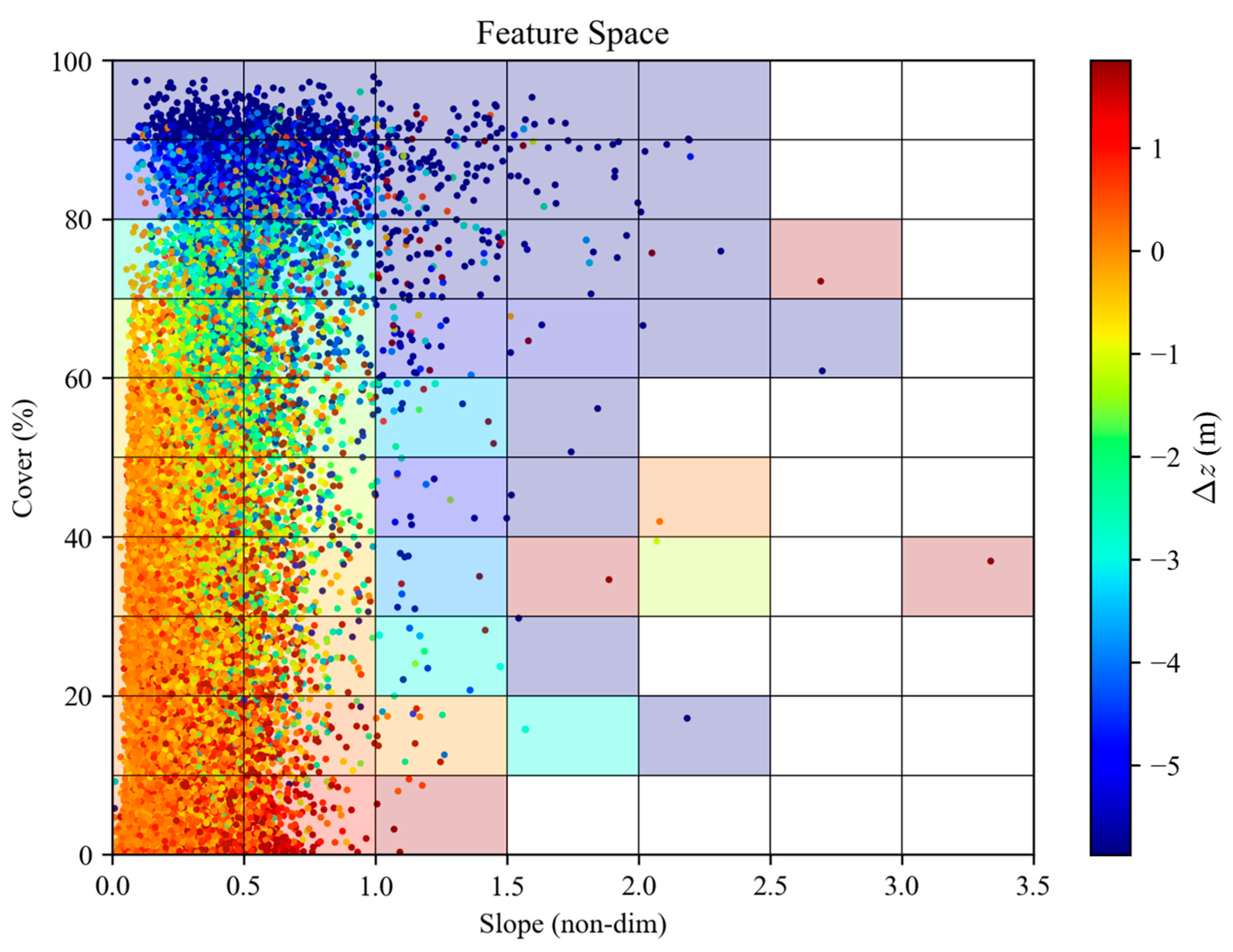
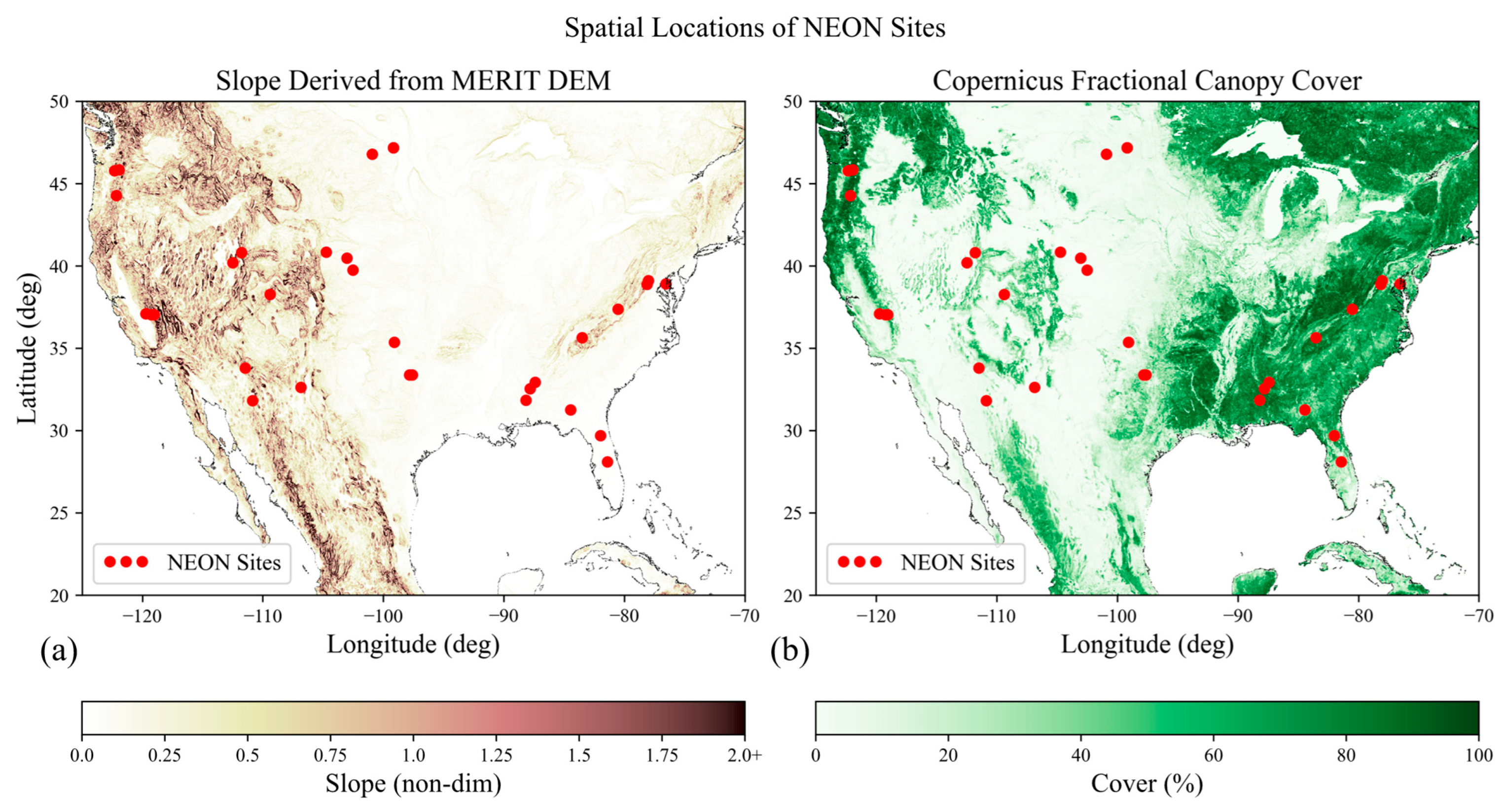
Out of 59 discrete return lidar sites, only 32 were selected, as 3 sites (BONA, DEJU, and HEAL) were outside latitudinal bounds of GEDI data and the rest did not have available data in the year 2021. Despite those sites out of range, 32 sites offer significant diversity in biomes across the United States [27,29,30]. Figure 1 shows how NEON sites are distributed in space over terrain slope and canopy cover features.

In Figure 1a, we downsampled the Multi-Error-Removed Improved-Terrain Digital Elevation Model (MERIT DEM) [33] to 1°/24, then derived demonstrative slope via a gradient, and scaled the slope to high-resolution slope obtained within each ROI. For Figure 1b, we performed a similar operation, downsampling the Copernicus Global Land Cover product [34] to 1°/25.2, and then averaged the value of cover for each pixel. The result is a demonstrative figure that shows where NEON ROIs are with respect to geographic features. Statistically, there are 10 ROIs with 90th percentile slope (S90) less than 0.25 and 90th percentile cover (C90) less than 50%; another 10 ROIs with S90 less than 0.25 but with C90 greater than 50%; 9 ROIs with S90 greater than 0.25 and C90 greater than 50%; and only 3 ROIs with S90 greater than 0.25 and C90 less than 50%.

2.3. GEDI L2B Data

GEDI launched in December 2018 and was positioned on the International Space Station (ISS) Japanese Experiment Module-Exposed Facility, which covers between ±51.6° latitude based on the ISS orbital inclination. The GEDI instrument provides multi-beam elevation measurements using three lasers. One “coverage” laser is split into two beams at 4.5 mJ each, which are dithered to produce four incident transects. The other two full “power” lasers are only dithered to produce an additional two transects, each at 15 mJ [27,35]. In total, there are 4 coverage and 4 power profiles (ground-tracks) on the surface of the Earth. Full power laser energy penetrates canopy cover more easily than the lower energy density of the coverage lasers, producing more ground detections, but not necessarily better terrain elevation accuracy than coverage beams [27]. The across-track spatial coverage of the resulting 8 beam profiles is 4.2 km, with ~600 m separation between beams [5]. Each of the GEDI lasers are produced at 1064 nm wavelength and provide a 25 m diameter footprint with 60 m along-track spatial resolution [5]. The full-waveform technology of the GEDI lidar allows the system to capture a complete temporal profile of the returned laser energy along the laser line-of-sight. This capability allows for retrieval of both vegetation structure, canopy metrics, and terrain elevation in most cases.

The GEDI science team derives many datasets and four level 2 data products from the measured full-waveform signal of each footprint. Datasets range from the waveform time-series (per footprint) on L1B to more refined products such as leaf area index (LAI) or canopy coverage on L2B. This study utilizes relevant L2B GEDI granules based on coincidence to NEON ROIs through the GEDI Finder tool for version 2 data. We used the VDatum v4.5 software (https://vdatum.noaa.gov/welcome.html, accessed on 28 October 2022) to convert longitude, latitude, and elevation to respective reference lidar projected coordinate systems.

Waveforms were filtered with the l2b_quality_flag, which removes returns obscured by clouds and background noise [36]. Variations in daytime or nighttime collection has not been shown to have a meaningful impact on terrain elevation accuracy [27]. Likewise, both power and coverage beams provide similar terrain elevation accuracy, where the ground signal is observable through canopy cover [27].

The GEDI horizontal geolocation error at the footprint level has a standard deviation of 10.2 m [37] and must be geocorrected before comparing against reference lidar to separate instrument performance from operationally induced errors. Waveform geolocation can be corrected through two primary techniques, waveform matching [29] and terrain matching [28,29]. In waveform matching, the full waveform profile from GEDI’s L1B product is compared against synthetic waveforms created from reference lidar, typically through the GEDI Simulator. The waveform geolocation is shifted horizontally until it agrees with the reference waveforms under a relevant matching criteria. We applied terrain matching instead, where a short segment (km-scale) of each beam track is shifted iteratively over a 1 m resolution reference lidar-based DTM until the mean absolute error (MAE) of elevations between the track and the DTM are minimized. We apply the same algorithm as the algorithm used to geocorrect ICESat-2 tracks in Refs. [38,39] through research correspondence. In our particular terrain matching technique, tracks are shifted by up to ±48 m in along- and cross-track directions, then compared to iteratively higher resolution DTMs made directly from the reference lidar. Resolutions iterate over 8 m, 4 m, 2 m, then 1 m, and for each resolution, we derive a correction estimate, then increase the resolution, and provide the prior correction as an initial condition for the next estimate. In this way, we robustly and efficiently geocorrect to 1 m resolution.

Applying the same terrain matching technique as ICESat-2 to GEDI could affect geocorrection quality, as ICESat-2 is a standalone satellite with much higher platform stability than the ISS, and the ICESat-2 footprint spacing is only 0.7 m as opposed to GEDI’s 60 m [4]. Schleich et al. [28] determined that, for GEDI, the along-track segment length should be lower than the structural vibration period of the ISS (1–10 s), choosing a segment length no lower than 13 footprints and no larger than 50 footprints (3 km, or 0.43 s of along-track motion). We initially processed 24 ROIs with no fewer than 10 footprints and <25 km segment lengths, and processed 8 ROIs with <5 km lengths, in light of the recent manuscript by Schleich et al. [28]. In post-processing, we found a systematic bias in 5 ROIs in particularly mountainous and forested terrain; upon re-processing at <5 km, much of the systematic errors were reduced. Through direct correspondence with the GEDI science team, it was suggested that we split tracks below the instrument jitter frequency, which is ~5 Hz, leading to track lengths of ~1.5 km. Upon reprocessing 3 different ROIs (TALL, GRSM, and SJER) at 1.5 km instead of 5 km, there were negligible differences in RERDs. This hypothesis is reinforced by the results of [28], which did not explore frequencies higher than 1 Hz but estimated geolocation accuracies similar to the waveform matching.

After estimating a horizontal geocorrection for every segment of each GEDI beam, we subtract out the vertical difference in elevation between the GEDI transect and the reference lidar, fully georectifying the GEDI beam transect with reference lidar in three dimensions. Then, we can finally determine the elevation residual, which is the remaining difference between geocorrected, range-corrected, measured GEDI elevations and the true elevation, approximated by reference lidar. That is, we separate the errors in GEDI elevation measurement from geolocation and ranging accuracy, and isolate errors only due to atmospheric effects, terrain characteristics, and vegetation structure.

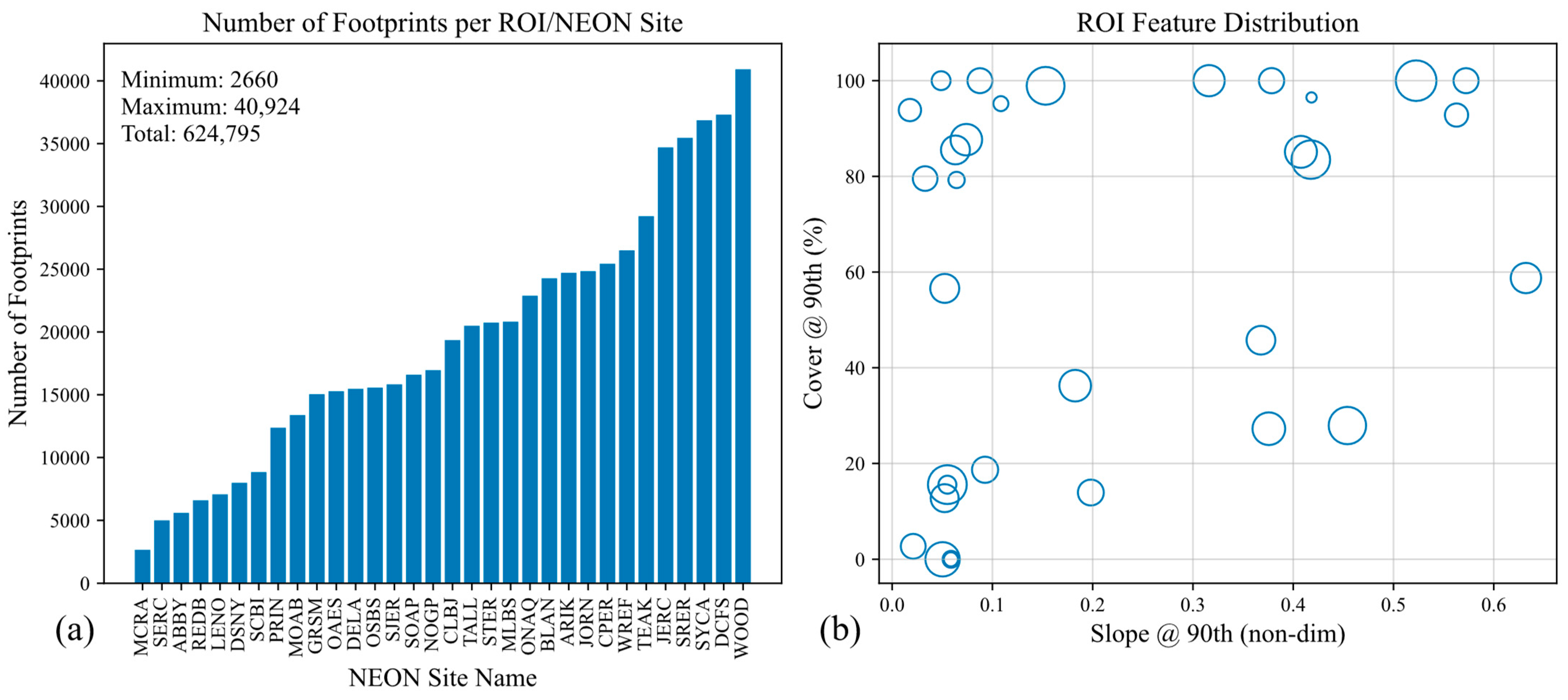
Processed data are filtered by quality footprints, whether there are more than 10–13 footprints in a “track”, and where the geocorrection algorithm diverged for a given track. Through all filters, we obtained 624,795 footprints to train the model. The smallest ROI has 2660 footprints while the largest has 40,924. Out of processed footprints, 48.2% are at daytime and 51.8% are at nighttime. In addition, 56.9% are from the power beam, while 43.1% are from the coverage beam.

2.4. Model Input Features

Numerous factors affect GEDI terrain elevation accuracy. Wang et al. [30] compiled a review of 9 studies since 2020, each focusing on factors influencing both terrain retrieval and relative canopy height accuracy. According to the extensive performance survey conducted by Liu et al. [27], in order of importance, the most impactful factors for terrain elevation retrieval are slope, canopy cover, canopy height, land cover type, and beam sensitivity. This study prioritizes the development of a general methodology that can scale to as many features (or factors influencing elevation residuals) as is necessary. As such, we have chosen the two most dominant features—terrain slope and canopy cover—to investigate elevation residual prediction.

Terrain slope—hereafter “slope”—is the tangent of the angle that terrain makes as it changes in elevation over a small area, with respect to both an x- and y-direction, such as along- and cross-track, or Easting and Northing in a Universal Transverse Mercator (UTM) projection. In a mathematical sense, slope is merely the magnitude of the gradient of the terrain surface. But in application to a real DTM, the calculation requires a user-specified “small area”. In the context of GEDI, the appropriate area size is the footprint, which is modeled as a circular disk with a diameter of 25 m projected vertically onto the DTM, centered on a geocorrected footprint geolocation.

Canopy fractional cover—or just “cover”—is equivalent to the percent of ground covered by a vertical projection of canopy material. The GEDI data product “cover” on L2B estimates cover, given leaves, branches, and stems [40]. As a feature, dense cover (e.g., in jungle/forest) correlates with lower terrain elevation accuracy because photons cannot pierce the canopy, resulting in a lower signal-to-noise ratio in ground detection.

While we can derive slope and cover from a reference DTM, the features are only applicable where reference data exists, preventing prediction elsewhere. Instead, we train the model on ancillary global feature datasets that are available at prediction. We derive slope through terrain elevation estimated by MERIT DEM [33]. The MERIT DEM is at 3 arcsecond resolution (~90 m at the equator) and covers latitudes from 60°S to 90°N, referenced to WGS84. The MERIT DEM is subset to the given ROI latitude and longitude bounds, then upsampled to 25 m (by interpolation) to reflect GEDI footprint size. Then, slope is derived by the gradient of the DEM, averaged over the GEDI footprint area. In this way, we extract a slope derived from MERIT per GEDI footprint. The incidence angle of each GEDI beam was not included because it was not mentioned in other works on GEDI terrain height validation vs. slope [27,30,41]. However, we understand it does have a slight impact on apparent slope. Upon comparing error distributions from reference-derived slope and MERIT-derived slope, we found that the inclusion of the incidence angle (limited to ~6°) is at or below the noise level in 90 m resolution MERIT. With more accurate features, we believe incidence angle will play a more meaningful role, but we do not believe it would have a significant impact on predictive capability in this work.

The process to extract canopy cover is similar, except we need not apply a post-processed gradient operation. Cover is represented by the Copernicus Global Land Cover product [34] “Tree_CoverFraction_layer” dataset for the year 2019, at ~3.6 arcsecond resolution (1°/1008), or ~100 m at the equator. The dataset extent is from 60°S to 78.25°N, and represents forest cover annually in 2019, the latest year available. The cover dataset is subset by the given ROI, upsampled to 25 m to coincide with GEDI footprint size. Then, cover is averaged over the GEDI footprint area. In this way, we extract the Copernicus forest canopy cover per GEDI footprint.

Slope is mostly temporally invariant, but canopy cover varies significantly by season. Unfortunately, there are not many high spatial and temporal resolution global canopy cover datasets available. “Cover” is a dataset on the GEDI L2B product that maps the exact forest cover to the GEDI footprint, which is spatially and temporally coincident. However, this is only applicable in training, and we cannot interpolate outside of the GEDI footprint measurements. Were a higher resolution, more temporally consistent canopy cover dataset to become available, we could replace the Copernicus forest cover in the year 2019 with a better feature dataset. The result is that the “cover” feature from Copernicus is less indicative of cover’s effect on elevation residual, as it would be with the GEDI L2B “cover” dataset.

Because the feature datasets are limited in latitudinal extent, our “global” predictive capability is limited to the overlap of the MERIT and Copernicus datasets, or 60°S to 78.25°N. While GEDI footprints only spatially cover 51.6° north and south, the feature space may cover further. That is, the model trained on slope and cover within ±51.6° may be indicative of slope and cover at higher/lower latitudes, assuming that slope and cover in other areas of the world are indicative of slope and cover within the U.S.-based NEON sites considered.

2.5. Theory

For a single point on Earth, there are only two scalar features (slope and cover), and the prediction, or target variable, is the entire ERD. The ERD quantifies the error of terrain elevation measurements—or the last peak of the waveform—not any other elements in the waveform. To be clear, the ERD is the culmination of the error in many thousands (or more) of ground returns and should not be confused with the distribution-like character of the return lidar waveform. If the ERD were modeled as a Gaussian distribution, we could parameterize the predictions as two scalars: mean and standard deviation. However, we found the Gaussian distribution to be insufficient for the accuracy required. In fact, the measured error (approximately true) distributions very closely resemble a Cauchy distribution. However, assuming Cauchy also introduced errors into prediction, we settled on a Gaussian mixture model (GMM).

Mathematically, the elevation residual is as follows:

$$\mathsf{\Delta }{z}_i=z_i-g\left({\stackrel{⃑}{p}}_i\right)$$

(1)

where $z_i$ is the $i$th measured ground elevation, $g$ is a function representing the reference DTM surface, ${\stackrel{⃑}{p}}_i$ is the geocorrected position in the reference coordinates, and $\mathsf{\Delta }{z}_i$ is the elevation residual. The elevation residual $\mathsf{\Delta }z$ (scalar) is modeled as a random process $f$, dependent on feature vector $x$:

$$\mathsf{\Delta }z~f\left(x\right)$$

(2)

For our study, $x=(m,c)$ is a feature pair of slope $m$ and canopy cover $c$. That is, for every slope and cover, we have a different distribution. If $f$ were Gaussian, the mean and standard deviation would change with respect to each feature pair. Note that $f$ does not depend on the spatial location, only slope and cover (or features in general).

Ultimately, the use case of our model is to predict how well GEDI retrieves elevation over a region, not just at a given point. Let $X$ be the set of all features in a given ROI. Then, through Monte-Carlo integration, the RERD is as follows:

$$f_{ROI}\left(\mathsf{\Delta }z;X\right)\approx \frac{1}{M}\sum _{\begin{array}{c}i=1\\ \end{array}}^{M}f\left(\mathsf{\Delta }z;x_i\right)$$

(3)

where $M=\left|X\right|$ is the number of feature points (or pairs) in the ROI (at training or prediction).

2.6. Model

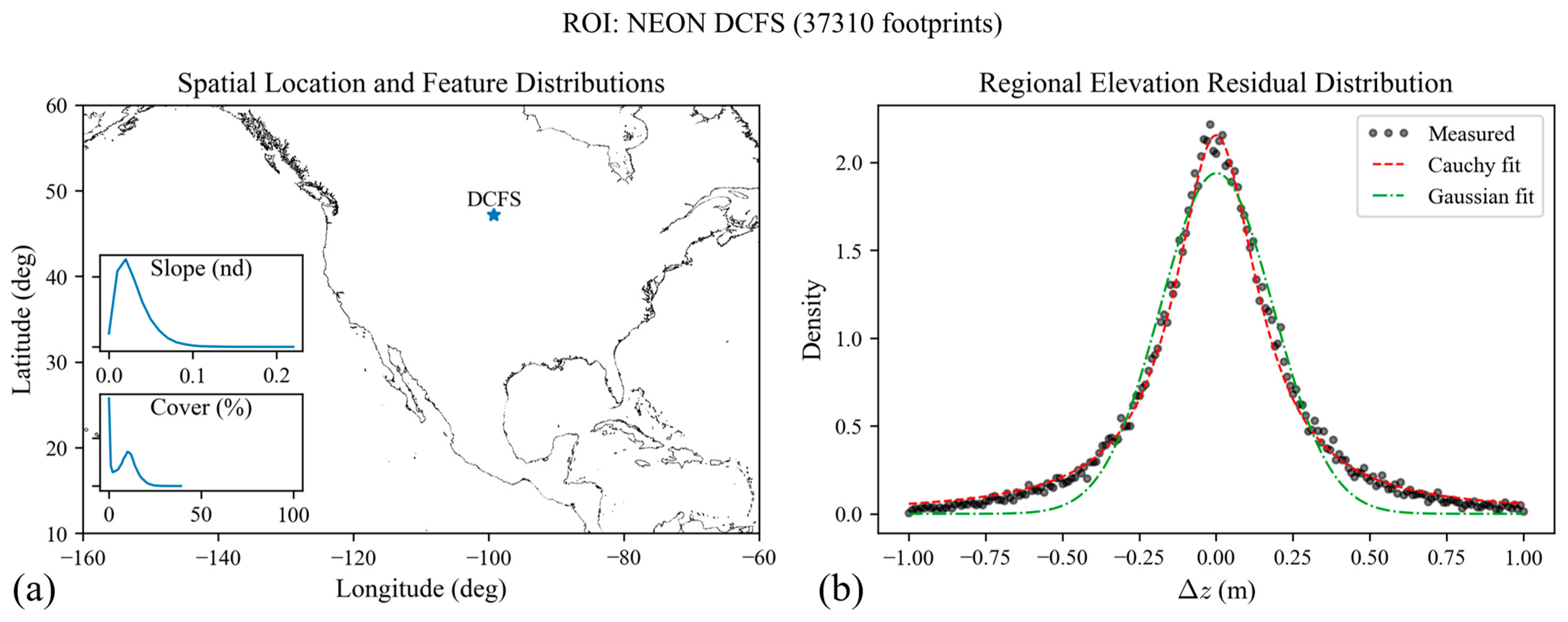
To clarify the model discussion, Figure 2 shows an example ROI (DCFS) including the spatial location of the ROI, feature distributions for slope and canopy cover, and the corresponding measured RERD directly from comparisons against the reference lidar. In addition, Figure 2 shows Cauchy and Gaussian fits of the RERD.

The RERD, or the ERD aggregated over the ROI, is built by a normalized histogram of all elevation residuals in the ROI, without respect to features. In Figure 2a, one can see “Slope” and “Cover” feature distributions. The key task is to correlate the distribution of slope and cover with the RERD, shown in Figure 2b, and ultimately predict a new RERD given the features in a new ROI.

A GMM can theoretically fit any distribution (given enough components), and it served as our baseline model, the MDN [24]. Expressing $f$ in terms of a GMM, we obtain the following equation:

$$f\left(\mathsf{\Delta }z;x\right)\approx \sum _{\begin{array}{c}j=1\\ \end{array}}^n{\alpha }_{j}N\left(\mathsf{\Delta }z;{\mu }_j,{\sigma }_j^2\right)$$

(4)

or $\mathsf{\Delta }z$ is distributed over $f$, dependent on a feature pair $x$, which is approximately equal to the weighted sum of $n$ Gaussian components; ${\alpha }_j$, ${\mu }_j$, and ${\sigma }_j$ are, respectively, the coefficient, the mean, and the standard deviation for the $j$th component. Explicitly, ${\alpha }_j$, ${\mu }_j$, and ${\sigma }_j$ are functions dependent on $x$.

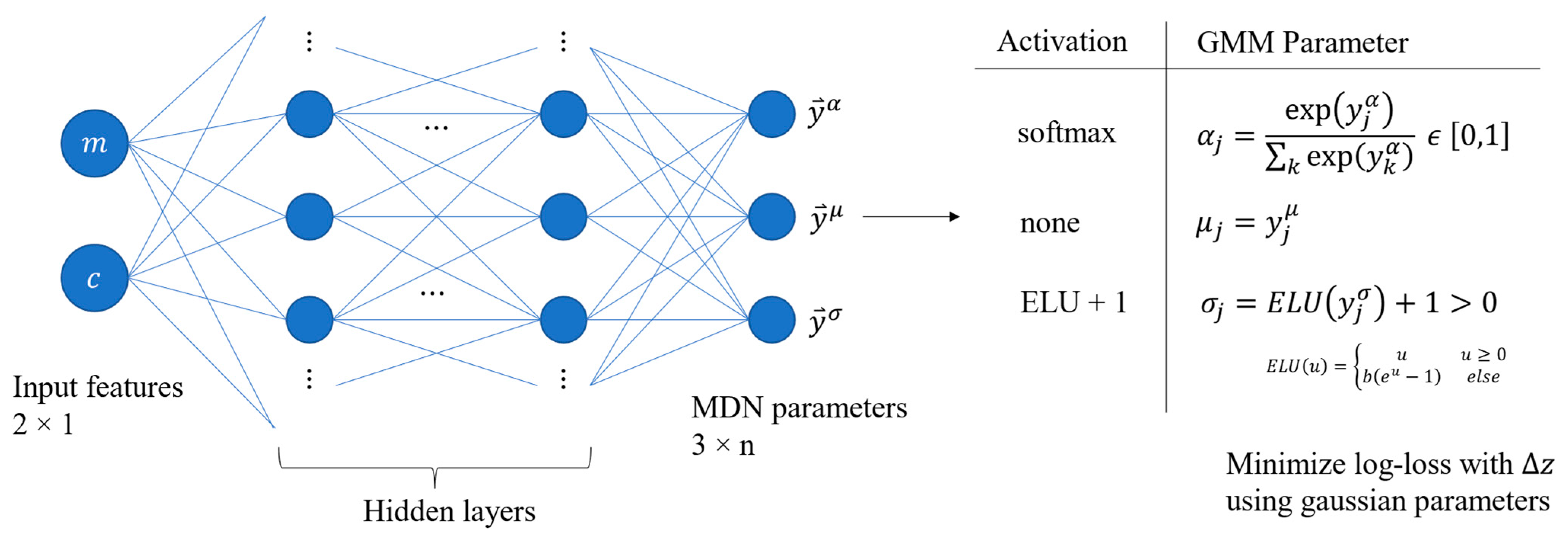
The MDN is a DNN with an output, mixture layer, that combines hidden layer outputs into coefficients, means, and standard deviations for the GMM. The MDN applied to our problem is shown in Figure 3.

The difference between the MDN and a traditional DNN is the addition of the output layer, and the corresponding selection of activation functions, shown in the table in Figure 3. The softmax activation is applied to ${\alpha }_j$ as the coefficients must sum to 1. The means have no constraints, and therefore no special activation function. The standard deviations must be positive. The activation was originally the exponential function [24] but was later adapted to the exponential linear unit (ELU) + 1 with unit slope ($b=1$ in Figure 3) [25], which exponentially approaches zero for the DNN output dummy variable $u<0$, and remains linear when $u\ge 0$. In this way, $\sigma$ predictions cannot diverge as easily, better conditioning the model. The loss function driving the MDN is the maximum likelihood of the negative log-loss of the GMM [24]:

$$L\left(\stackrel{⃑}{\theta }\right)=-\frac{1}{M_T}\sum _{i=1}^{M_T}\log \left(\sum _{j=1}^n{\alpha }_{ij}N\left(\mathsf{\Delta }{z}_i;{\mu }_{ij},{\sigma }_{ij}^2\right)\right)$$

(5)

where $\stackrel{⃑}{\theta }$ is a vector of 3$n$ GMM parameters, including all $\alpha$, $\mu$, and $\sigma$ over all components, computed over all training features $M_T$. Note that realizations $\mathsf{\Delta }{z}_i$ (training data) are input instead of the elevation residual axis, $\mathsf{\Delta }z$.

After all components in $\stackrel{⃑}{\theta }$ are estimated (the model is trained), we have the capability to predict at footprint-scale through Equation (4), or equivalently, through $f$. However, the RERD is of more importance to our study. Combining Equation (4) with Equation (3), the aggregate prediction is as follows:

$$\begin{array}{c}{f}_{ROI}\left(\mathsf{\Delta }z;X_P\right)\approx \frac{1}{M_P}{\displaystyle \sum _{i=1}^{M_P}}{\displaystyle \sum _{\begin{array}{c}j=1\\ \end{array}}^n}{\alpha }_{ij}N\left(\mathsf{\Delta }z;{\mu }_{ij},{\sigma }_{ij}^2\right)\end{array}$$

(6)

or $\mathsf{\Delta }z$ is distributed over the RERD prediction $f_{ROI}$, given all prediction features in the ROI $X_P$ ($M_p=\left|X_P\right|$), which is approximately equal to the aggregate of Gaussian mixtures at every feature point in the ROI.

The MDN can predict an entire distribution over an arbitrary region, but from a mission planning perspective, the distribution is not as important as whether elevation residuals fall within a confidence interval threshold. For example, mission planners might specify that “90% of elevation residuals shall be within ±2 m.” Then, we can specify the elevation threshold $\mathsf{\Delta }{z}_0$ (e.g., 2 m), and the percentage of elevation residuals within a predicted RERD that meet mission requirements is as follows:

$$P_{\mathsf{\Delta }z}=\mathrm{Pr}\left(\left|\mathsf{\Delta }z\right|<\mathsf{\Delta }{z}_0|X_p\right)={\int }_{\begin{array}{c}-\Delta z_0\\ \end{array}}^{\mathsf{\Delta }{z}_0}{f}_{ROI}\left(\mathsf{\Delta }z;X_P\right)\mathsf{\Delta }z$$

(7)

or the probability that elevation residuals $\mathsf{\Delta }z$ are within the mission threshold $\mathsf{\Delta }{z}_0$, based on the new prediction ROI features $X_p$, is equal to the integral over the predicted RERD in the new ROI. In short, we quantify this confidence interval as $P_{\mathsf{\Delta }z}$, which is directly informative in terms of mission requirements.

2.7. Training and Prediction

Training directly on quality footprints from each ROI can introduce bias in the model if the ROIs are not equally weighted. Figure 4 shows how the number of measurements is significantly different from one ROI to another. To balance the occurrences of the elevation residual per ROI, we set a maximum number of training points to the total number of footprints available (624,795 samples), then uniformly sample each ROI dataset equally. In this way, ROIs are represented equally in training.

About half (19/32) of the measured RERDs have a mode of nearly zero (<1 cm), but some ROIs with large slopes and dense canopy cover reached modes of up to 7 cm. If the geocorrection pipeline were perfect, we should see modes of zero. We attribute the error to the culmination of segment length, geocorrection resolution of 1 m, potential misclassifications in reference ground signal at the base of trees, and temporal differences between NEON and the GEDI footprints. For a worst-case ROI (GRSM), we reduced the maximum segment length from 25 km to 5 km, and the corresponding mode offset changed from 21 cm to 7 cm, supporting the hypothesis that mode offsets are due to processing errors, not the true GEDI elevation residual. Therefore, before training on any elevation residuals, we fit a Cauchy distribution to the observed RERD, and subtract the mode of the peak from all elevation residuals in the ROI, thereby removing processing errors from measured elevation residuals.

The model is trained by splitting the elevation residuals and features into training and testing sets, with 80% and 20% of the data, respectively. To determine the hyperparameters to train on, we performed a k-fold cross-validation. Because we are ultimately predicting RERDs, we split total data sets by ROI during cross-validation, not by footprint. For example, with a 5-fold cross-validation, the first fold may contain 25 ROIs of data and another 7 ROIs are set aside for validation. We then train on 80% of the 25 ROIs, predict on 20% of the same 25 ROIs to fit the model, then compare new predictions against the 7 holdout ROIs for validation. In this way, we determine how the model generalizes to data it has not seen. Because we have a sparse set of ROIs (only 32), a uniformly random split across all the ROIs could produce models that are not trained on significant portions of the feature space; therefore, we performed a k-fold cross-validation with random selection over subsets of the feature space.

Table 1. Cross-validation subset distribution.

Quadrant	Slope (Non-Dim)	Cover (%)	Number of ROIs
1	>0.25	>50	9
2	<0.25	>50	10
3	<0.25	<50	10
4	>0.25	<50	3

lists the distribution of ROIs per feature subset.

For each k-fold, we randomly select 2 ROIs from quadrants 1–3 and randomly select 1 ROI from quadrant 4 as test ROIs (7 total), then train on the rest.

We compare predictions to the measured RERD to tune the model, using the Jensen–Shannon Divergence (JSD) [42], which can be defined by the average of the Kullback–Liebler (KL) divergence $D_{KL}$ between two distributions $P$ and $Q$:

$$JSD\left(P\left|\right|Q\right)=\frac{1}{\begin{array}{c}2\\ \end{array}}{D}_{KL}\left(P\left|\right|R\right)+\frac{1}{2}{D}_{KL}\left(Q\left|\right|R\right)$$

(8)

$$R=\frac{1}{\begin{array}{c}2\\ \end{array}}\left(P+Q\right)$$

(9)

The combination gives a “measure of the total divergence to the average distribution” [43], where, in our case, $P$ is the measured RERD and $Q$ is the predicted RERD.

We set the number of hidden layers to 2 with 100 neurons each. We used the python package TensorFlow to implement a DNN and modified it to fit the MDN structure, using the Adam optimizer. Then we applied a grid-search-based 5-fold cross-validation to vary the number of Gaussian components over (3, 5, 7, 10), batch size over (64, 128, 256), and learning rate over (0.1, 0.01, 0.001, 0.0001).

During training and cross-validation, we randomly sampled each ROI to preserve feature diversity while maintaining a sufficiently high number of training and prediction samples. We predict through Equations (6) and (7). However, on a global scale, prediction becomes computationally intractable. Relative to feature space, it is not vital to aggregate predictions for every single feature pair in a new ROI. Instead, to predict at scale, we downsample the feature space in a new ROI, predicting on weighted feature bins instead of individual feature points, approximating the RERD prediction (Appendix A).

2.8. Method Summary

Summarizing training, we performed the following tasks:

• Chose and downloaded 32 NEON reference lidar sites;
• Downloaded GEDI L2B version 2 granules over those sites and extracted quality footprints;
• Geocorrected GEDI L2B footprints with DTMs built from ground classified NEON reference lidar;
• Difference geocorrected elevations with DTMs to obtain elevation residuals;
• Extracted slope derived from MERIT DEM and canopy cover from Copernicus over each NEON site;
• Removed mode/processing bias in RERDs from measured elevation residuals;
• Trained the MDN, correlating slope and cover to elevation residual.

Summarizing the regional prediction, we performed the following tasks:

• Chose a user-defined ROI somewhere on Earth within 60°S to 78.25°N;
• Extracted slope derived from MERIT DEM and canopy cover from Copernicus over the new ROI;
• Downsampled the feature space into weighted feature bins for faster prediction;
• Predicted on weighted feature bins, obtaining approximate GMM parameters;
• Aggregated all predicted GMMs over the new ROI.

3. Results

3.1. Model Validation and Accuracy

To train the model, we minimize the negative log-loss of the GMM. To optimally choose hyperparameters in the cross-validation, we minimize the JSD between the predicted and measured RERDs. The JSD was minimized to 0.0098 for seven mixture components, with a batch size of sixty-four and a learning rate of 0.001. Divergence is a convenient measure of how different a predicted distribution is from a validation (or measured) distribution. However, divergence is not easily interpretable in terms of model accuracy. The model assumes a non-Gaussian distribution, but we can present accuracy in terms of an “equivalent standard deviation” ${\sigma }_{EQ}$ or the standard deviation of a Gaussian fit to the measured or predicted distributions. In this regard, we model with no Gaussian assumption, but present cross-validation prediction accuracy in a way that is more easily understood. Note that our prediction variable is not a kind of mean; rather, it is a type of variance (through the predicted distribution), because we are quantifying uncertainty in the GEDI elevation retrieval. It would not make sense to present results on an “equivalent mean” because the predicted mean is always nearly zero, because we estimate only the error in the georectified elevation measurement. In

Table 2. Cross-validation error statistics.

Row	Error Type	Using All Feature Points	Using Feature Bins
A	Average error in ${\sigma }_{EQ}$	−0.06 m	−0.04 m
B	Standard deviation of ${\sigma }_{EQ}$	0.18 m	0.19 m
C	Average of relative error of ${\sigma }_{EQ}$	15.9%	26.7%

, we present the cross-validation prediction accuracy over all folds.

In Table 2 row A, we show that the mean of the difference in ${\sigma }_{EQ}$ of our predictions vs. the measured data is −0.06 m, with no feature bin downsampling. That is, our ${\sigma }_{EQ}$ prediction is consistent with the measured RERDs. In Table 2 row B, we evaluate the standard deviation of our predicted ${\sigma }_{EQ}$, which is 0.18 m. That is, we may, on average, predict ${\sigma }_{EQ}$ with a 6 cm bias, but the true error may vary between ±18 cm at 1$\sigma$. And finally, in Table 2 row C, we show the relative error of our prediction for ${\sigma }_{EQ}$, which is 15.9%, or our prediction of ${\sigma }_{EQ}$ is off, on average, by 15.9%. In the last column, we instead predict by downsampling the dataset in feature space (Appendix A). Rows A and B remain consistent, but row C is increased because there are several predicted distributions that have small variance (in flat, semi-barren areas), and with a lower prediction accuracy due feature binning, their relative error is high. Because the Table 2 results are based on cross-validation, the values are representative of generalization error.

Alternatively, we look at the in-sample relative error of ${\sigma }_{EQ}$ by ROI. That is, we train on all data, and test on all data to conduct an intercomparison of each ROI’s relative error, shown in Figure 5.

Figure 5 shows the relative error change across the feature space for each ROI. In addition, we have highlighted three different ROIs at high slope and high canopy cover: WREF, MCRA, and GRSM, with slope, cover, and RERDs on the left side of Figure 5. The relative error of GRSM is 50.2%, but WREF and MCRA are 21.1% and 43.7%, respectively. The RERD of GRSM nearly matches that of MCRA, but the slope and canopy cover of MCRA is higher. According to slope and cover, the model predicts GRSM as a sharper distribution than is measured, more similar to WREF. Likely, slope and canopy cover are not enough to quantify the variation in GRSM vs. MCRA. Similarly, nine other ROIs are predicted with relative error in excess of 25% throughout the feature space. The outlier error suggests that the model is not overfitting the training data and that the error is likely a result of predicting from only two features and generalizing the model during cross-validation.

In light of the errors, we exchanged the cover feature for the GEDI L2B cover dataset to predict in-sample errors, using the same cross-validated model hyperparameters, as a quantitative investigation. The ROI GRSM relative error reduced from 50.2% to 30.3%. WREF increased by 7.5% to 28.7% relative error, and MCRA reduced by 30.1% to 13.6% relative error. The average relative error remained similar to Table 2 row C, at 16.3%, implying that outlier ROIs are predicted better given the higher-quality cover. While 72% (23/32) of ROIs are within 25% relative error given the cover derived from Copernicus, this comparison against the GEDI cover dataset indicates that the Copernicus cover dataset—and the choice of only two features—is insufficient to reliably predict mountainous, forested regions at meter-scale elevation error.

3.2. Global Validation in Localized Areas

We performed a localized quantitative validation on the prediction accuracy of $P_{\mathsf{\Delta }z}$ over a range of $\mathsf{\Delta }{z}_0ϵ\left[\mathrm{0.1,3}\right]$ m, for locations in France, Hawaii, New Zealand, and Puerto Rico. In France, we acquired reference lidar from The Institut National de L’information for a ~10 × 10 km² plot near Moirans-en-Montagne in eastern France, collected in the summer of 2023 [44]. The French dataset is referenced to the Reseau Geodesique Francaise 1993 datum, with the GRS 1980 ellipsoid. For Hawaii, we acquired the NEON PUUM dataset for January 2020 (with the same reference system as the other NEON sites). We chose the Tasman district in New Zealand, with surveys conducted by Toitū Te Whenua Land Information New Zealand between January 2020 and January 2022. We acquired the reference lidar through OpenTopography [45]. The New Zealand site is referenced to the New Zealand Transverse Mercator 2000 coordinate system, with the NZVD2016 vertical datum, over the GRS 1980 ellipsoid. The Puerto Rico dataset was also available through NEON as the GUAN site, which we acquired for May 2018. We filtered and geocorrected GEDI L2B footprints in the same manner as that used to create the training data (all at 5 km segment lengths).

In Figure 6, we show the difference error between the true $P_{\mathsf{\Delta }z}$ and the predicted $P_{\mathsf{\Delta }z}$, for France, Hawaii, New Zealand, and Puerto Rico ROIs, along with their respective locations in feature space as compared to the training data. In addition, we show in-sample errors in gray lines, which represent a lower bound on how accurate we should expect $P_{\mathsf{\Delta }z}$ to be, assuming that predictions over the trained set will typically be more accurate than those outside of the trained set. In

Table 3. True and predicted global validation of $P_{\mathsf{\Delta }z}$.

ROI	Num. Footprints	${\mathit{P}}_{\mathsf{\Delta }\mathit{z}} {\left.\right|}_{\mathsf{\Delta }{\mathit{z}}_0=1}$ (%)	${\mathit{P}}_{\mathsf{\Delta }\mathit{z}} {\left.\right|}_{\mathsf{\Delta }{\mathit{z}}_0=3}$ (%)	Relative Error of ${\mathit{\sigma }}_{\mathit{E}\mathit{Q}}$ (%)
France	20,873	51.9	78.6	42.0
Hawaii	10,208	61.7	90.0	58.2
New Zealand	20,139	26.3	56.0	49.5
Puerto Rico	8928	60.8	84.4	54.1

, we show the number of footprints per ROI, the true $P_{\mathsf{\Delta }z}$ given $\mathsf{\Delta }{z}_0=1\mathrm{m}$, the true $P_{\mathsf{\Delta }z}$ given $\mathsf{\Delta }{z}_0=3\mathrm{m}$, and the relative error of the equivalent standard deviation as compared to the prediction.

The error analysis of $P_{\mathsf{\Delta }z}$ is not as straightforward as ${\sigma }_{EQ}$ because $P_{\mathsf{\Delta }z}$ is a percentage, so we ensured that our “difference error” in Figure 6a is simply the predicted $P_{\mathsf{\Delta }z}$ minus the true (measured) $P_{\mathsf{\Delta }z}$ from the reference lidar and real L2B footprints. Even so, the value of $P_{\mathsf{\Delta }z}$ changes as a function of $\mathsf{\Delta }{z}_0$. If, for example, $\mathsf{\Delta }{z}_0=0\mathrm{m}$, then we are predicting the percent of elevation residuals within 0 m—which is trivially zero. On the other end, we can also attempt to predict the percent of elevation residuals within 10 m (or a value $\gg$3 m), which will be ~100%. These two edge-cases are simple to predict and have correspondingly small prediction errors. However, in-between the two extremes, there is an interval of $\mathsf{\Delta }{z}_0$ where the error will be maximum, depending on the width of the true RERD. When the RERD is thin (or ${\sigma }_{EQ}$ is small, e.g., flat, vegetation-free areas), the error in $P_{\mathsf{\Delta }z}$ reduces quickly because 3 m is considered “large” for such an RERD. In areas where the RERD is wider (${\sigma }_{EQ}$ is large, e.g., mountainous and forested areas), 3 m may not be as large, relatively, as is the case for New Zealand in Figure 6a. The interpretation of the difference error must also be scrutinized because one cannot say, “$P_{\mathsf{\Delta }z}$ is typically in error of 10%”, because there are locations on Earth and values of $\mathsf{\Delta }{z}_0$ that make $P_{\mathsf{\Delta }z}>90\%$, which would result in a prediction above 100%.

However, we can form some intuition about the accuracy of $P_{\mathsf{\Delta }z}$ by inspecting both Figure 6 and Table 3. For France, $P_{\mathsf{\Delta }z}{\left.\right|}_{\mathsf{\Delta }{z}_0=1}$ is 51.9%, but the MDN overestimates by about 10.2%. For $P_{\mathsf{\Delta }z}{\left.\right|}_{\mathsf{\Delta }z=3}$ = 78.6%, the MDN overestimates by 5.3%. In Hawaii, for 1 m and 3 m, it overestimated by 22.0% and 5.0% for a true $P_{\mathsf{\Delta }z}$ of 61.7% and 90.0%, respectively. For New Zealand, it overestimated by 12.2% and 12.0% for a true $P_{\mathsf{\Delta }z}$ at 26.3% and 56.0%, respectively. And finally, in Puerto Rico, the MDN overestimated by 14.7% for 1 m and 6.8% for 3 m, for a true $P_{\mathsf{\Delta }z}$ of 60.8% and 84.4%, respectively. The Hawaii ROI is of particular interest because it is less accurate than New Zealand (even with ${\sigma }_{EQ}$ in Table 3), despite being relatively flat, and in-between training sets in feature space, shown in Figure 6b. The MDN should interpolate well for Hawaii, but the results show otherwise, which heavily indicates that Copernicus and MERIT features in Hawaii do not properly account for the observed elevation residuals.

Relatively, the error in $P_{\mathsf{\Delta }z}$ is always higher for $\mathsf{\Delta }{z}_0=1\mathrm{m}$. In general, predictions made with $\mathsf{\Delta }{z}_0=3\mathrm{m}$ are more reliable because there is less potential for elevation residuals in general to veer beyond 3 m. In a relative sense, predicting $P_{\mathsf{\Delta }z}$ is typically more accurate than ${\sigma }_{EQ}$ for two reasons: (1) ${\sigma }_{EQ}$ is a derived quantity from fitting a Gaussian distribution to predicted RERDs and $P_{\mathsf{\Delta }z}$ is integrated analytically from the predicted GMM via Equation (7); and (2) $P_{\mathsf{\Delta }z}$ predictions have a natural decrease in error for relatively extreme bounds of $\mathsf{\Delta }{z}_0$, which does not decrease the validity of the predictions but rather their application; a unit-based uncertainty metric like ${\sigma }_{EQ}$ is applicable in other contexts, whereas $P_{\mathsf{\Delta }z}$ serves the unique goal of mission requirement compliance. Conceptually, increasing $\mathsf{\Delta }{z}_0$ increases the relative accuracy but at the expense of prediction resolution. As a basic takeaway, if $\mathsf{\Delta }{z}_0$ is ~1 m, we may see errors in $P_{\mathsf{\Delta }z}$ on the order of 5–30%, and if $\mathsf{\Delta }{z}_0$ is ~3 m, we may see errors on the order of 5–15%, depending on the slope and cover of the region.

3.3. Application: Global Prediction

The presented methodology offers a technique to predict the error in GEDI-like elevation measurement from a footprint to global scale, given clear-sky conditions. As an example application, we predict $P_{\mathsf{\Delta }z}$ at 0.25 × 0.25 deg. resolution globally (60°S to 78.25°N). We first predict $P_{\mathsf{\Delta }z}$ at 10 × 10 km² in the sinusoidal equal area projection, which produces unbiased statistics regardless of latitude [46], then resample outputs to 0.25 × 0.25 deg. resolution on a latitude–longitude geographic projection with the WGS84 ellipsoid. In addition, because MERIT DEM includes inland lakes and rivers, we masked $P_{\mathsf{\Delta }t}$ outputs by resampled Ocean and Permanent Water Bodies classifications at 0.25 × 0.25 deg. from the Copernicus Moderate Dynamic Land Cover 100 m dataset (version 3) [34].

In Figure 7, we show $P_{\mathsf{\Delta }z}$ from 60°S to 78.25°N for $\mathsf{\Delta }{z}_0$ = 1 m and $\mathsf{\Delta }{z}_0$ = 3 m. For $\mathsf{\Delta }{z}_0$ = 1 m, the lower 10th percentile of $P_{\mathsf{\Delta }z}$ is 60.7%, the median is 88.5%, and the 90th percentile is 96.6%. For $\mathsf{\Delta }{z}_0$ = 3 m, the lower 10th percentile of $P_{\mathsf{\Delta }z}$ is 83.4%, the median is 96.4%, and the 90th percentile is 99.3%. In Figure 7a, $\mathsf{\Delta }{z}_0$ = 1 m, and there are mountainous areas such as the Rocky Mountains, Himalayas, and the Andes Mountains, where the percent of elevation residuals within 1 m is ~50%. Further, in areas of dense vegetation, $P_{\mathsf{\Delta }z}$ is also quite low, such as throughout the equatorial latitudes in South America, Africa, and Indonesia. In Figure 7b, $\mathsf{\Delta }{z}_0$ = 3 m, so there is more room for elevation error, and $P_{\mathsf{\Delta }z}$ is in general much higher than in Figure 7a. That is, it is much more likely that elevation residuals are within 3 m than 1 m. And in flatter, barren regions, $P_{\mathsf{\Delta }z}$ is high for both cases. These trends follow the qualitative understanding that, in regions with high slopes and dense cover, geocorrected elevation retrieval has more error.

4. Discussion

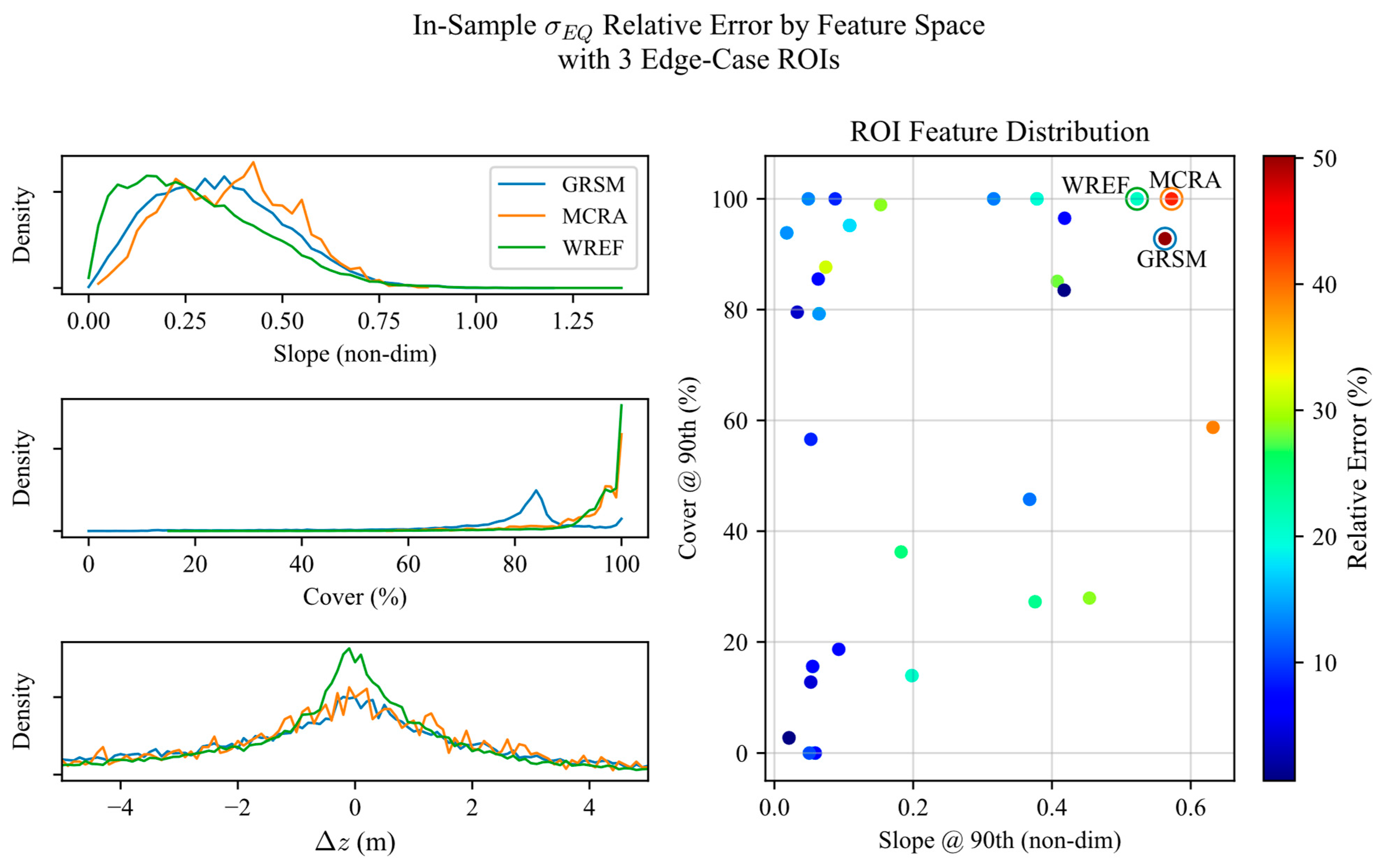
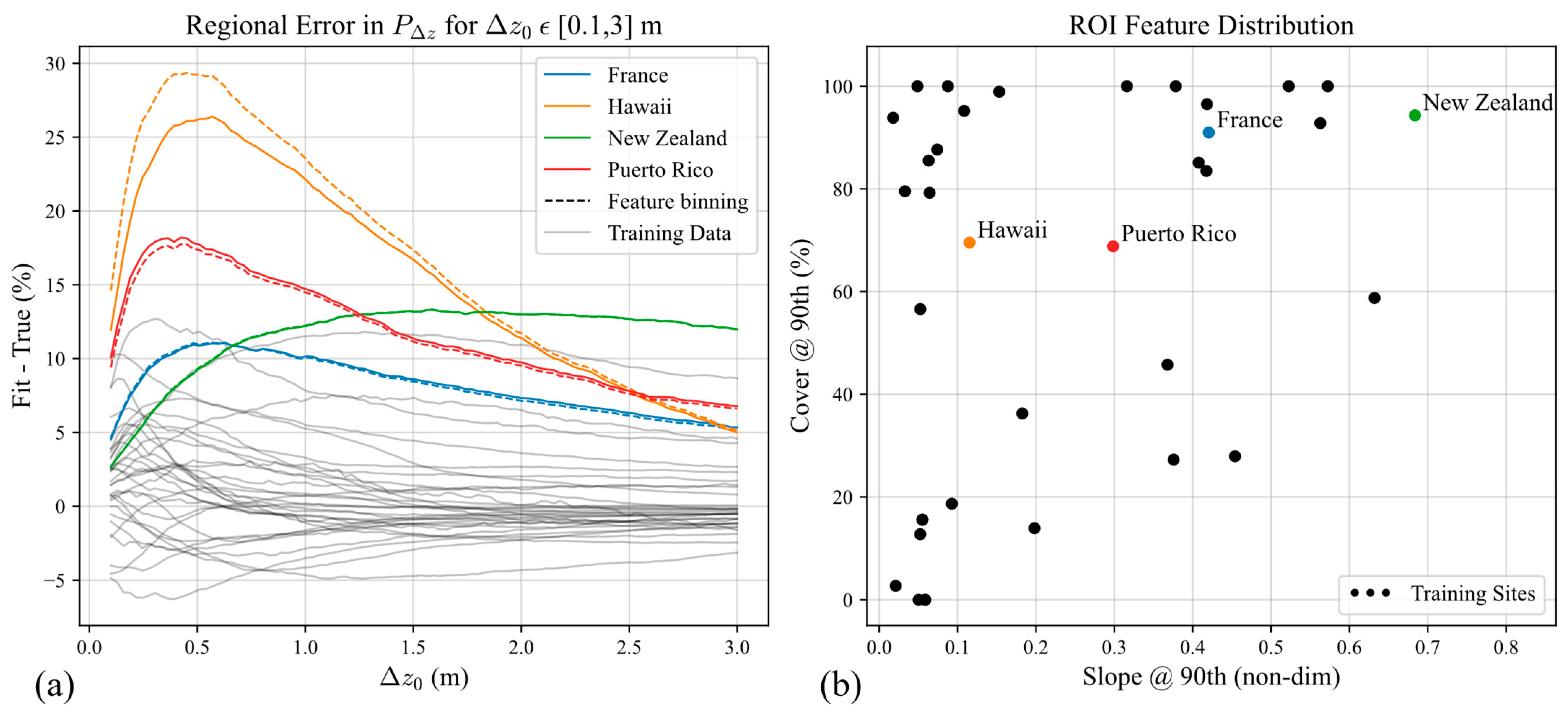
We have trained the MDN at the footprint scale and developed a statistical technique through feature binning to predict at the global scale while remaining computationally feasible. Through the cross-validation results, predicting from only slope and canopy cover features has a 15.9% mean relative error of ${\sigma }_{EQ}$. From in-sample analyses, the MDN predicts for flat, barren areas with less than a 25% relative error of ${\sigma }_{EQ}$. For more mountainous and forested regions, the relative error can reach 50.2%. When validated against sites outside the U.S., relative errors of ${\sigma }_{EQ}$ were from 42.0 to 58.2%. The error is understandable considering that only average forest canopy cover is used from the Copernicus 2019 dataset. Furthermore, GEDI footprints are not filtered by leaf on/leaf off conditions and footprints are queried from 2019 through 2021. Canopy cover could be enhanced by including Moderate Resolution Imaging Spectroradiometer (MODIS) and Landsat tree cover datasets [47,48], which are on the GEDI L2B data product per footprint (for training) and available at the global scale via external datasets for prediction. Potentially, a low spatial resolution canopy cover with a higher temporal resolution might sufficiently supplement a high spatial resolution canopy cover dataset, effectively breaking temporal and spatial cover into separate features. MERIT DEM-derived slope is likely sufficient and is clearly impactful to the global prediction; however, it could be supported by other external terrain datasets, such as the Forest and Buildings Removed Digital Elevation Model (FABDEM) [49], which is at 30 m resolution instead of MERIT’s 90 m resolution. Besides terrain slope and canopy cover, there are other factors that influence GEDI elevation measurement fidelity, such as land cover type, solar illumination, and beam sensitivity [27], and the MDN predictions would likely fare better by including these features.

While the ${\sigma }_{EQ}$ relative errors are somewhat high, the true value of ${\sigma }_{EQ}$ is on the order of ~1 m, and a 50% relative error translates to a 0.5–1.5 m prediction. The benefit of ${\sigma }_{EQ}$ is that it is an easily understandable accuracy metric, but the drawback is that the RERDs are non-Gaussian, and we must derive ${\sigma }_{EQ}$ from fits of the measured and predicted distributions, which introduces artifacts to this highly sensitive parameter. $P_{\mathsf{\Delta }z}$, on the other hand, is less interpretable, but is derived from measured elevation residuals with a simple percentage calculation and derived from the predicted distributions analytically since the prediction is a sum of Gaussians. Therefore, $P_{\mathsf{\Delta }z}$ has no artifacts. In addition, it has a scalable resolution through $\mathsf{\Delta }{z}_0$, which simultaneously makes it more informative for the exact elevation residual distribution, and less clear because the $P_{\mathsf{\Delta }z}$ error changes by region and the $\mathsf{\Delta }{z}_0$ bound in question.

After discussion with the GEDI science team, a few more minor elements, if implemented in a future work, would increase the fidelity of predictions:

• The off-nadir angle of each beam (which is at maximum around ~6°) should be included in the slope determination, as it is the apparent terrain slope that leads to variation in elevation uncertainty, not the terrain slope. Retrieving the apparent slope is not exactly straightforward, as the pointing vector itself is not on a GEDI product but is instead parameterized in the elevation and azimuth angles of the incident unit vector. One can derive the apparent slope angle through the dot product between the surface normal and the incident unit vector [35,50]. The apparent slope itself is then the arctangent of the slope angle.
• There is a high-frequency jitter component in the GEDI tracks at about ~5 Hz. The recommended track lengths are around 1.5 km, below that of [28], which suggested 3 km. However, Schleich et. al.’s suggestions were based on track lengths that are short enough to accommodate high-frequency components of pointing, while long enough to guarantee valid solutions in terrain matching, which depends on the number of footprints. In the post-analysis, we found that track lengths of 1.5 km for TALL, SJER, and GRSM ROIs slightly flattened out elevation residual measurements at higher slopes, indicating that predictions would fare better with a model trained on the shorter track lengths. We hypothesize that shorter track lengths are more sensitive to instrument jitter for regions with higher slopes, which have enough topography to terrain match properly. Longer track lengths may be usable in flatter terrain, where elevation measurement error is not as susceptible to high-frequency jitter.
• The L2B degrade_flag, which indicates orbit, pointing, and timing-based degrades, is independent of the l2b_quality_flag, and could indicate where geolocation is poor despite having valid waveforms.

Our feature set does not explain the predicted residuals well, and a change of slopes by up to ~6°, or reduction in track lengths to reduce noise in higher slopes, or the inclusion of a degrade flag would not compensate for a poorly observed target variable. However, coupled with more features in a follow-up study, any model trained on GEDI should include those minor adjustments, as small errors in preprocessing would become more dominant in a more precise prediction.

While the MDN is an effective choice to model a GMM, it is somewhat heavy for the task of predicting a univariate, Cauchy-like distribution. Experimenting with Gaussian and Cauchy distribution models, we found them in much more error than the GMM. It may be preferable to apply a linear regression to predict the mean absolute error of ROIs instead of the entire RERD itself. With a simpler model, predictions could be faster, and the model could be less prone to overfitting. Or, instead of training at the footprint scale and aggregating distributions to predict regionally, one can directly train ${\sigma }_{EQ}$ regionally. The drawback is that predictions may be fixed to only the spatial scale trained on, whereas the intent of the MDN strategy is the applicability to a wide response domain, such as predictions of elevation residual quality from footprints to continents.

5. Conclusions

This study has shown how to map slope and canopy cover to clear-sky measured elevation error for a spaceborne, 1064 nm, 25 m-footprint full-waveform lidar. Relative to the understanding that GEDI elevation residuals should be more accurate in flatter, barren areas, and less accurate in mountainous, forested areas, the MDN provides a coarse predictive capability given the limited feature set. From the results of Figure 6a, we can see that slope and canopy cover in the U.S. are not very indicative of slope and canopy cover elsewhere in the world, at least as derived from MERIT DEM and Copernicus canopy cover, and with respect to predicting the elevation residual. While the predictions are somewhat poor, we believe the technique can offer a way to model uncertainty, given a richer feature diversity and a refined preprocessing pipeline.