Automatic Targetless Monocular Camera and LiDAR External Parameter Calibration Method for Mobile Robots

Abstract

With the continuous development and popularization of sensor-fusion technology for mobile robots, the application of camera and light detection and ranging (LiDAR) fusion perception has become particularly important. Moreover, the calibration of extrinsic parameters between the camera and LiDAR is a crucial prerequisite for fusion. Although traditional target-based calibration methods have been widely adopted, their cumbersome operation and high costs necessitate the development of more efficient and flexible calibration methods. To address this problem, this study proposed a two-stage calibration method based on motion and edge matching. In the first stage, the preliminary estimation of the extrinsic parameters between the camera and LiDAR was performed by matching visual odometry and LiDAR odometry using a hand–eye target method. In the second stage, the calibration results from the first stage were further refined by matching the image edges and discontinuous depth point clouds. The calibration system was then tested in both simulated and actual environments. The experimental results showed that this method, which did not require specially structured targets, could achieve highly flexible and robust automated calibration. Compared to other advanced methods, the accuracy of the proposed method was higher.

1. Introduction

With the rapid development of robots, artificial intelligence, and multi-sensor fusion perception technologies, the perception capabilities of mobile robots have greatly expanded, resulting in more convenient, intelligent, and safe equipment, such as unmanned vehicles and aerial drones [1,2]. Similar to the “eyes” of robots, vision sensors play an important role in environmental perception. However, in a complex environment, the data acquired by a single sensor cannot satisfy the necessary requirements. Consequently, mobile robots are equipped with multiple sensors. As mainstream visual sensors, cameras and light detection and ranging (LiDAR) sensors complement each other in terms of providing information, so their fusion can overcome their limitations and improve their environmental perception abilities.

Robots with visual and LiDAR perception have been widely used in important fields such as target detection and tracking [3,4,5], self-driving [6,7,8,9], indoor navigation [10], and simultaneous localization and mapping (SLAM) [11,12,13,14]. However, the extrinsic parameters of different sensors must be determined before they can be effectively fused. Extrinsic calibration is the process of estimating the rigid-body transformation between the reference coordinate systems of two sensors and is a prerequisite for many scene-based applications. In the field of target detection and tracking, by obtaining the extrinsic parameters between the camera and LiDAR sensor, the data from the two can be aligned in the same coordinate system to achieve multi-sensor fusion target detection and tracking tasks, thereby improving tracking accuracy. In the field of 3D reconstruction [15,16,17], obtaining an accurate spatial relationship between the two is conducive to obtaining richer and more accurate 3D scene information. Combining the high-precision 3D information from the LiDAR sensor and the RGB information from the camera ensures more efficient and reliable 3D reconstruction results. Additionally, extrinsic calibration between the camera and LiDAR sensor is an important preliminary step in visual–LiDAR fusion SLAM. For example, visual–LiDAR odometry and mapping (VLOAM) [11] combines the visual information of a monocular camera with that of the LOAM. To perform visual–LiDAR fusion SLAM, the spatial calibration between the two sensors must be determined. The extrinsic parameters between the camera and LiDAR sensor provide important prior information to the system, accelerating backend optimization, while the LiDAR sensor can supplement the scale loss of monocular vision to provide more complete spatial information and correct motion drift.

In recent years, scholars have proposed several methods for the joint calibration of cameras and LiDAR. In traditional camera and LiDAR calibration, the calibration objects are typically observed simultaneously using sensors [18,19]. Moreover, these methods focus on various designs for calibrating the objects and algorithms that match them. However, extracting the corresponding features from a calibrated object can be difficult. Special calibration sites are required, which can be extremely vulnerable to artificial and noise interference. By contrast, motion-based calibration methods can automatically estimate the extrinsic parameters between cameras and LiDAR sensors without requiring structured targets; however, their calibration accuracy needs to be further improved [20].

In this study, we propose a targetless calibration method that could be applied to mobile robot sensor systems. The contributions of this study are as follows:

• We propose a two-stage calibration method based on motion and edge features that could achieve the flexible and accurate calibration of cameras and LiDAR sensors in general environmental scenes.
• We designed an objective function that could recover the scale factor of visual odometry while achieving the initial estimation of extrinsic parameters, providing a good initial value for the fine calibration stage.
• Experiments were conducted on both simulated and real-world scenes to validate the proposed method. Compared with other state-of-the-art methods, the proposed method demonstrated advantages in terms of flexibility and accuracy.

The remainder of this paper is organized as follows. Section 2 reviews the research status of scholars in this field. Section 3 describes the workflow of the proposed method. Section 4 provides a detailed description of the research methods and optimization techniques. Section 5 introduces the experimental setup in both simulation and real-world scenarios and presents the results of various experiments and visualizations. Section 6 discusses the experimental results and their rationale. Finally, Section 7 concludes the study.

2. Related Work

Currently, the calibration methods for LiDAR sensors and cameras can be categorized into two groups, that is, target-based and targetless methods. Target-based methods involve the use of specific calibration targets during the calibration process to extract and match features, thereby obtaining the extrinsic parameters between the cameras and LiDAR sensor. Zhang et al. [21] calibrated the internal parameters of cameras and LiDAR sensors using a chessboard pattern and obtained their extrinsic parameters. Because of their clear planar features and advantages—such as their high accuracy, ease of implementation, and good stability—the use of chessboard patterns has been extensively studied [22,23,24,25,26]. Cai et al. [27] customized a chessboard calibration device that provided local gradient depth information and plane orientation angle information, thereby improving calibration accuracy and stability. Tóth et al. [28] used a smooth sphere to solve the extrinsic parameters between the cameras and LiDAR sensors by calculating the corresponding relationship between the sphere centers. Beltrán et al. [29] proposed a calibration method that could be applied to various combinations of monocular cameras, stereo cameras, and LiDAR sensors. They designed a special calibration device with four holes, which provided shared features for calibration and calculated the extrinsic parameters between different sensors. In summary, the advantages of such calibration methods are their high accuracy and being able to design different calibration targets for different application scenarios. However, target-based methods require special equipment and complex processes, resulting in increased costs and complexity.

However, targetless methods do not require specific targets during the calibration process. Instead, they statistically analyze and model the spatial or textural information in the environment to calculate the extrinsic parameters between the cameras and LiDAR sensors [30]. Targetless methods can be roughly classified into four groups, that is, information-theoretic, motion-based, feature-based, and deep-learning methods. Information-theoretic methods estimate the extrinsic parameters by maximizing the similarity transformation between cameras and LiDAR sensors [20,31]. Pandey et al. [32] used the correlation between camera image pixel grayscale values and LiDAR point-cloud reflectivity to optimize the estimation of extrinsic parameters by maximizing the mutual information. However, this method was sensitive to factors such as environmental illumination, leading to unstable calibration results.

Motion-based methods solve the extrinsic parameters by matching odometry or recovering the structure from motion (SfM) during the common motion of the cameras and LiDAR sensors. Ishikawa et al. [33] used sensor-extracted odometry information and applied a hand–eye calibration framework for odometry matching. Huang et al. [34] used the Gauss–Helmert model to constrain the motion between sensors and achieve joint optimization of extrinsic parameters and trajectory errors, thereby improving the calibration accuracy. Wang et al. [35] computed 3D points in sequential images using the SfM algorithm, registered them with LiDAR points using the iterative closest point (ICP) algorithm, and calculated the initial extrinsic parameters. Next, the LiDAR point clouds were projected onto a 2D plane, and fine-grained extrinsic parameters were obtained through 2D–2D edge feature matching. This method had the advantages of rapid calibration, low cost, and strong linearity; however, the estimation of sensor motion often exhibited large errors, resulting in lower calibration accuracy.

Feature-based calibration methods calculate the spatial relationship between the camera images and LiDAR point clouds by extracting common features. Levinson et al. [36] calibrated the correspondence between an image and point-cloud edges, assuming that depth-discontinuous LiDAR points were closer to the image edges. This calibration method has been continuously improved [37,38,39] and is characterized by high accuracy and independence from illumination. It is commonly used in online calibration.

Deep-learning-based methods use neural-network models to extract feature vectors from camera images and LiDAR point clouds, which can then be input into multilayer neural networks to fit the corresponding extrinsic parameters. This method requires a considerable amount of training and has high environmental requirements; therefore, it has not been widely used [40]. In summary, these methods have the advantages of a simple calibration process, no requirement for additional calibration devices, and rapid calibration performance. However, in complex environments with uneven lighting or occlusions, the calibration accuracy can be diminished.

In certain application scenarios—such as autonomous vehicles—more extensive calibration scenes and efficient automated calibration methods are required. Consequently, we proposed a targetless two-stage calibration strategy that enabled automatic calibration during motion in natural scenes while ensuring a certain degree of calibration accuracy.

3. Workflow Overview of the Proposed Method

This section introduces a method for the joint calibration of the camera and LiDAR sensor. Figure 1 shows the proposed camera–LiDAR joint calibration workflow.

In the first stage, the camera and LiDAR sensors synchronously collect odometric information and motion trajectories. Specifically, the camera motion trajectory is obtained by visual odometry based on feature extraction and matching [41], whereas the LiDAR motion trajectory is obtained from edge point-cloud registration-based LiDAR odometry [42]. Based on the timestamps of the LiDAR motion trajectory, the camera poses are interpolated, and new odometry information is used to construct a hand–eye calibration model to estimate the initial extrinsic parameters. In the second stage, calibration is performed by aligning the edge features in the environment. By finding the minimum inverse distance from the projected edge 3D point cloud to the 2D camera edge image given the initial extrinsic parameters of the camera and LiDAR sensor, an optimization strategy combining the basin-hopping [43] and Nelder–Mead [44] algorithms can be used to refine their extrinsic parameters.

4. Methodology

In this section, we elaborate on the proposed camera–LiDAR joint calibration method based on motion and edge features.

4.1. Initial External Parameter Estimation

The camera and LiDAR sensors were fixed on a unified movable platform, their relative positions remaining unchanged. However, there was no direct correspondence between the observations of the two sensors. Consequently, the motion of each sensor had to be estimated simultaneously, the motion trajectories being used to calculate the extrinsic parameters between the camera and the LiDAR sensor. This method is a hand–eye calibration model, as shown in Figure 2. The mathematical model can be expressed as $T_L^a{T}_{LC}=T_{LC}{T}_C^a$, where $T_L^a$ denotes the pose transformation information of the LiDAR from timestamp $t_a$ to $t_{a+1}$, $T_C^a$ denotes the pose transformation information of the camera from $t_a$ to $t_{a+1}$, and $T_{LC}$ denotes the transformation parameter from the LiDAR coordinate system to the camera coordinate system, that is, the extrinsic parameter.

In the calibration process, the primary task is to estimate the motion of each sensor. The monocular visual odometry method in ORB-SLAM [41] was used for camera motion estimation. Its front-end includes feature extraction, feature matching, and pose estimation modules. By tracking feature points, it can calculate the camera motion trajectory in real time and return the motion trajectory in the form of rotational angles. The LOAM algorithm [42] was used for LiDAR motion estimation. By matching the edge and plane features in the point cloud, we could obtain a set of consecutive relative pose transformations and return them as rotation angles.

Because the number of frames for the camera and LiDAR trajectories do not correspond one to one, preprocessing of the two odometry datasets is required. Among them, we utilized the concept of Spherical Linear Interpolation (Slerp) to construct novel trajectories. Specifically, we assumed that the timestamp of a certain LiDAR frame was $t$, satisfying $t_a<t<t_{a+1}$, where $t_a$ and $t_{a+1}$ were the timestamps of two adjacent camera pose frames, with poses denoted by $T\left(t_a\right)$ and $T\left(t_{a+1}\right)$. We used $\frac{\left(t-t_{\mathrm{a}}\right)}{t_{\mathrm{a}+1}-t_{\mathrm{a}}}$ as the interpolation coefficient to estimate the new position and orientation. The interpolated camera position and orientation at time $t$ can be calculated as follows:

$$T\left(t\right)=T\left(t_{\mathrm{a}}\right)+\frac{\left(T\left(t_{\mathrm{a}+1}\right)-T\left(t_{\mathrm{a}}\right)\right)\left(t-t_{\mathrm{a}}\right)}{t_{\mathrm{a}+1}-t_{\mathrm{a}}}$$

(1)

Using Equation (1) with the LiDAR trajectory timestamps as a reference, all camera pose frames can be interpolated to obtain a new camera trajectory. Once the LiDAR trajectory $T_L^i\in \left\{T_L^1,T_L^2,\cdots ,T_L^k\right\}$ and the corresponding camera trajectory $T_C^i\in \left\{T_C^1,T_C^2,\cdots ,T_C^k\right\}$ are determined, based on the hand–eye calibration model, we can obtain:

$$R_L^{i}R=R{R}_C^i$$

(2)

$$R_L^{i}t+t_L^i=R{t}_C^i+t$$

(3)

where $R$ and $t$ denote the extrinsic parameter matrices between the camera and LiDAR sensor.

Because monocular visual odometry has scale ambiguity, there exists a scale $s$ between $T_L^i$ and $T_C^i$. Introducing the scale factor $s$ allows for scaling the positional relationship between the camera and the LiDAR to align it with the scale in the real world. Consequently, multiplying the translation terms in Equation (3) using the unknown scale $s$ gives:

$$R_L^{i}t+t_L^i=R{t}_C^i·s+t$$

(4)

Because the correct rotation matrix is orthogonal, based on orthogonality, $R^{T}R=I_{3\times 3}$, where $I_{3\times 3}$ is a 3 $\times$ 3 identity matrix. Using the orthogonality of the rotation matrix as a constraint, the extrinsic parameter solution can be converted into an optimization problem with equality constraints, as follows:

$$\underset{R^{*},t^{*},s}{\min }{\displaystyle \sum }_{i=1}^k(\Vert R_L^i{R}^{*}-R^{*}{R}_C^i\Vert {}^2+\mu \Vert R_L^i{t}^{*}+t_L^i-R^{*}{t}_C^i·s-t^{*}\Vert {}^2),$$

(5)

where $\mu$ denotes a weighting parameter used to balance the influence between the two objective functions.

The pure equality constrained optimization problem in Equation (5) can be solved using the sequential quadratic programming (SQP) method with the joint iterative optimization of the extrinsic parameters $R^{*}$, $t^{*}$, and scale $s$. The essence of the SQP algorithm lies in transforming the optimization problem with equality constraints into a quadratic programming sub-problem and iteratively updating the Lagrange multipliers to optimize the objective function. This approach effectively handles equality constraints and exhibits a certain level of global convergence. When the change in the objective function value is below a certain threshold, the algorithm converges, and a relatively accurate initial extrinsic parameter ${\xi }^{\prime }$ can be obtained. ${\xi }^{\prime }$ can also be calculated using the inverse Rodrigues formula, providing important initial guidance for the subsequent refinement calibration stage.

4.2. Refined External Parameter Estimation

A calibration method based on motion can be realized by matching the odometry information. However, because the sensor continuously moves without loop closure detection, the pose information inevitably accumulates errors, limiting the accuracy of the calibration results. Specifically, there may also be potential errors in the mis-synchronization between visual and LiDAR odometers. To enhance the quality of the extrinsic parameter calibration, an edge-matching method was employed to further optimize the extrinsic parameters. The proposed method can be divided into two modules. In the first module, edge features of the image and discontinuous depth points from the LiDAR channel data are extracted, preparing for the subsequent edge-matching task. In the second module, discontinuous depth points are projected onto a plane using the camera’s intrinsic parameter ($K$) and initial extrinsic parameters. The camera’s intrinsic parameter matrix $K$, which includes the focal length, principal point, and image coordinate origin, was derived from calibration data provided by the device manufacturer. We believed that the camera’s intrinsic parameter matrix $K$ was reliable. Ultimately, an optimization algorithm minimizes the distance between the edge images, thereby achieving refined extrinsic parameters.

4.2.1. Edge Feature Extraction

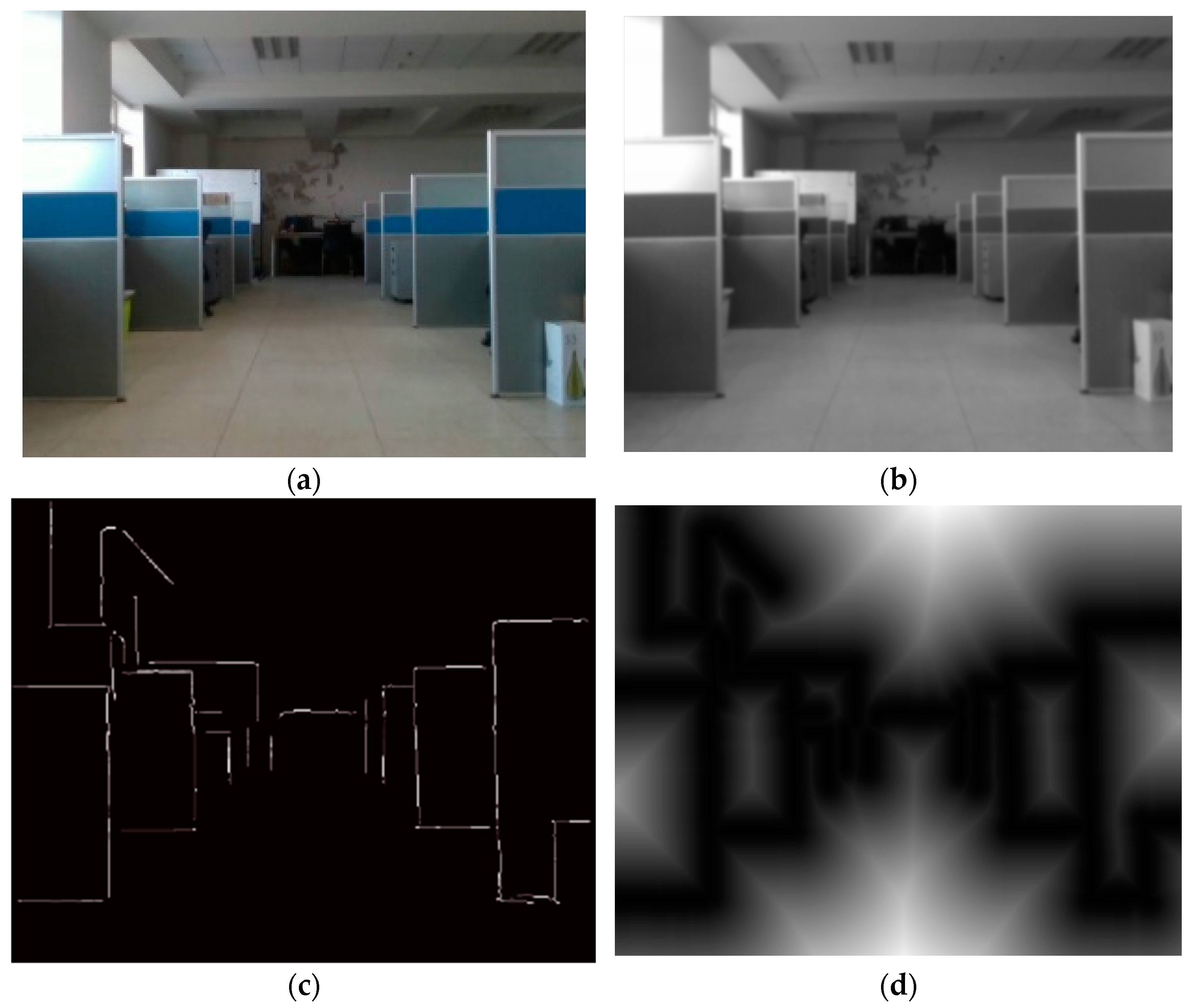
For the synchronized sample data obtained from different scenarios, a series of processing steps must be performed on the images and point clouds to extract common edge features from the scenes. Because image and point-cloud edge feature extractions are performed separately, the specific processing methods are explained below.

Edge features in images typically appear in regions with substantial changes in pixel values. Hence, the classic Canny algorithm [45] was adopted in this study to detect the image edge features using the edge extraction scheme shown in Figure 3. First, Gaussian filtering was applied to smooth regions with weak edge features. We increased the kernel size to reduce unnecessary image edge features. By doing so, our objective is to focus on the most relevant and distinctive edge features for calibration while minimizing the impact of noise and irrelevant details to the maximum extent possible. Subsequently, non-maximum suppression and double thresholding were used to retain strong edge points with local maxima and suppress the surrounding noisy points. In this article, we set the high threshold to 1.7 times the low threshold. Finally, the broken-edge features are connected via the Hough transform to generate an edge binary mask. These steps can effectively filter out minor edges and retain significant edges, resulting in improved performance.

To encourage alignment of the edge features, a distance transform [46] can be applied to the edge binary mask to extend the radius of the edges. The closer it is to the edge, the stronger the edge energy. In subsequent edge-matching optimization, the distance-transformed image facilitates smooth pixel-wise matching and avoids becoming stuck in a local optimum.

For point-cloud processing, considering the depth differences between individual LiDAR channel points, a point-cloud depth-discontinuity method [36] can be used to extract the edge point clouds. This method detects locations with considerable depth changes in the point cloud to extract edge information. Based on the sequence number of the LiDAR channel to which each point belongs, LiDAR points are assigned to the corresponding channel ($c_i$) in sequential order, where $i$ denotes the number of LiDAR channels. The depth value ($d_{i,j}$) of each point in every channel can then be calculated along with the depth difference between each point and its adjacent left and right points, as follows:

$$d_j=\max \left(d_{i,j-1}-d_{i,j},d_{i,j+1}-d_{i,j},0\right)$$

(6)

At this point, each point $p_j$ is assigned a depth difference value ($d_j$). Based on our testing experience, we consider a depth difference exceeding 50 cm as an edge point. All points identified as edges are aggregated into a point cloud, as shown in Figure 4b.

4.2.2. External Parameter Calibration for Edge Feature Matching

As described in the previous section, the depth-discontinuity method obtains the edge point cloud ($P_i^L$). To project this onto the image plane, the initial extrinsic parameters from the first stage can be used. The projected pixel coordinates of $P_i^L$ on the image plane can be calculated as follows:

$${[u_i^L,v_i^L,1]}^T=K\left(R^{*}{P}_i^L+t^{*}\right),M={\left\{1,\dots ,m\right\}}_{i=1}$$

(7)

where $K$ denotes the intrinsic camera matrix, $R^{*}$ denotes the initial rotation matrix, and $t^{*}$ denotes the initial translation vector.

The pixel points obtained from Equation (7) can be used to generate a binary mask projected onto the image to obtain the binary image ($G_i^L$). Combined with the distance-transformed edge mask ($G^C$) described in Section 4.2.1, the average chamfer distance between the two edge features can be calculated. This converts the extrinsic calibration into an optimization problem that minimizes the chamfer distance, which can be expressed as follows:

$$\underset{\xi }{\min }\frac{1}{m}{\displaystyle \sum }_{i\in M}{G}_i^L\odot G^C,$$

(8)

where ⨀ denotes the Hadamard product, $G_i^L$ denotes the binary mask formed by the edge point cloud, and $\xi$ denotes the vector form of the extrinsic parameters.

Redundancy often exists in image edges, resulting in a non-one-to-one correspondence between the 2D edges. Consequently, multiple solutions may exist for this problem. Additionally, when $G^L$ is far from the radiation range of $G^C$, correct gradient guidance is lacking, and it can be easy to get stuck in a local minimum. In this study, we employed a hybrid optimization strategy that combines the basin-hopping and Nelder–Mead algorithms. The basin-hopping algorithm was utilized to identify the optimal region within the global context. By introducing random perturbations around the initial estimated external parameters, it enables continuous jumps and searches for the global optimal solution. Then, the Nelder–Mead algorithm was used to find the local optima within the optimal region until the distance was minimized. This integrated approach effectively balances the requirements of global exploration and local refinement, thereby enhancing the precision of the optimization parameters. The extrinsic parameters at this point could be considered to be the final optimized results.

5. Experimental Results

In this section, we first introduce the sensor system of the movable robot platform and then list the main sensor configurations.

Virtual calibration scenarios were built on a virtual simulation platform, and simulation sensor systems were constructed based on real sensor parameters. Qualitative and quantitative evaluations of the proposed calibration method were then conducted using simulations and real experiments. We experimentally compared the accuracy of the motion-based, manual point selection, and mutual-information calibration methods. Additionally, point-cloud projection results were demonstrated under different scenarios. Using this experimental design, the flexibility of the proposed calibration method and accuracy of the results could be demonstrated.

5.1. Setup

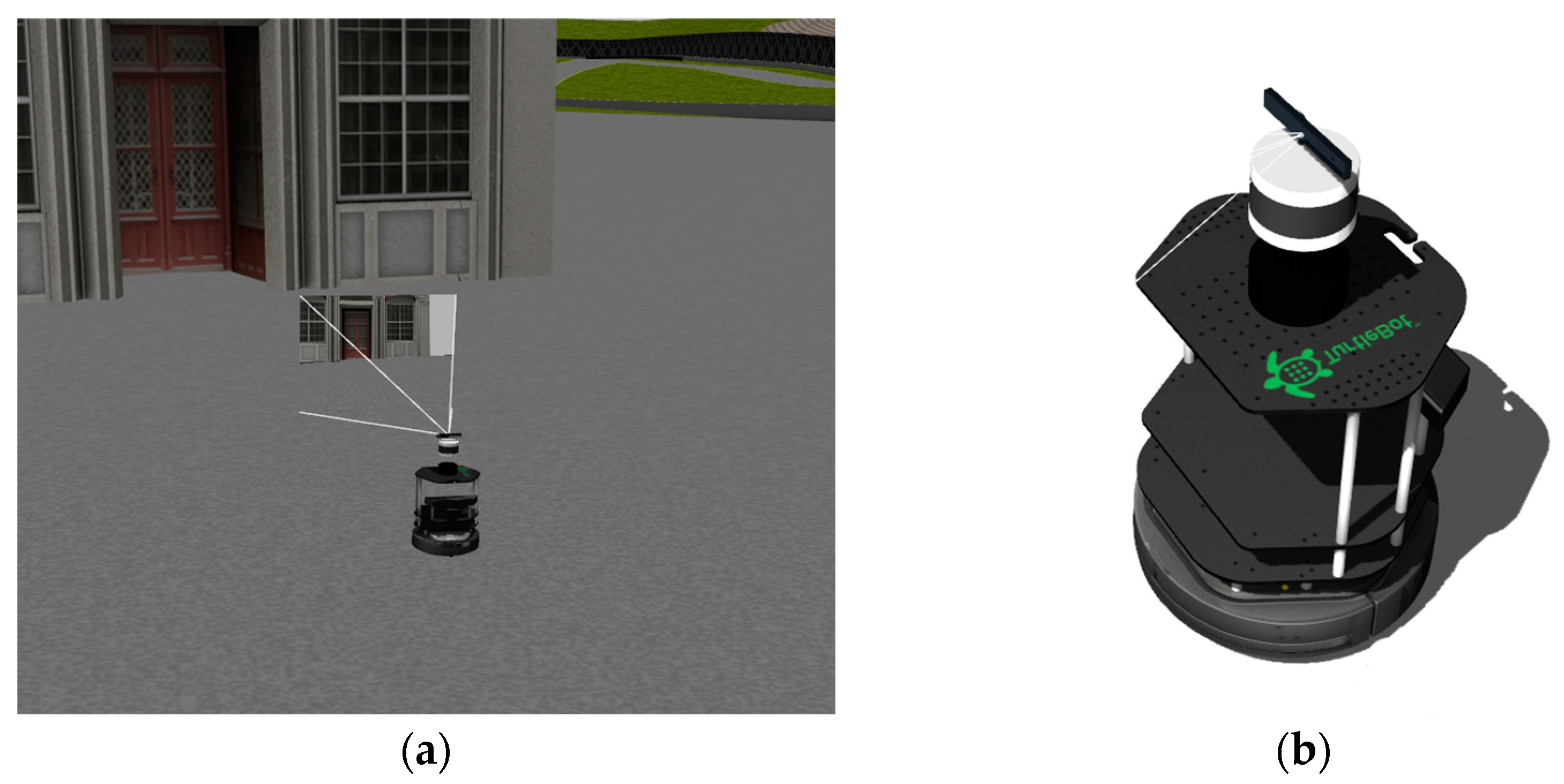
The multi-sensor platform used in this study is shown in Figure 5a. A 32-line Velodyne VLP-32C mechanical LiDAR system is installed at the top of the platform, as shown in Figure 5b. It has an observation range of up to 200 m, a 360° horizontal field of view (FOV), a 40° vertical FOV, and a rotational frequency of 20 Hz. Below the LiDAR sensor is a RealSense D435 camera with a 640 × 480 resolution in monocular mode, 25 mm fixed focal length, 30 fps frame rate, and a sensor FOV of 69° × 42°. The robot operating system (ROS) was used with Ubuntu 16.04.

Figure 6 shows the environment and sensor settings used in the simulation experiment. In this study, the Gazebo simulation platform was used to build a calibration environment rich in objects. The simulated camera and LiDAR sensors are associated with a unified TurtleBot2 robotic platform. The parameters of the LiDAR sensor and camera were set based on the real sensor specifications. After launching the corresponding nodes, the robot could be controlled through the ROS to collect data during motion.

5.2. Simulation Experiment

The camera and LiDAR sensor were installed on the TurtleBot2 robotic platform. By controlling the robot with commands to move in different directions, this experiment performed circular trajectory motions to excite movements in multiple orientations while simultaneously recording data from the camera and LiDAR sensor [33]. By extracting odometry information, 1100 frames of pose data could be randomly selected for the initial extrinsic calibration. The model converged after 20 iterations.

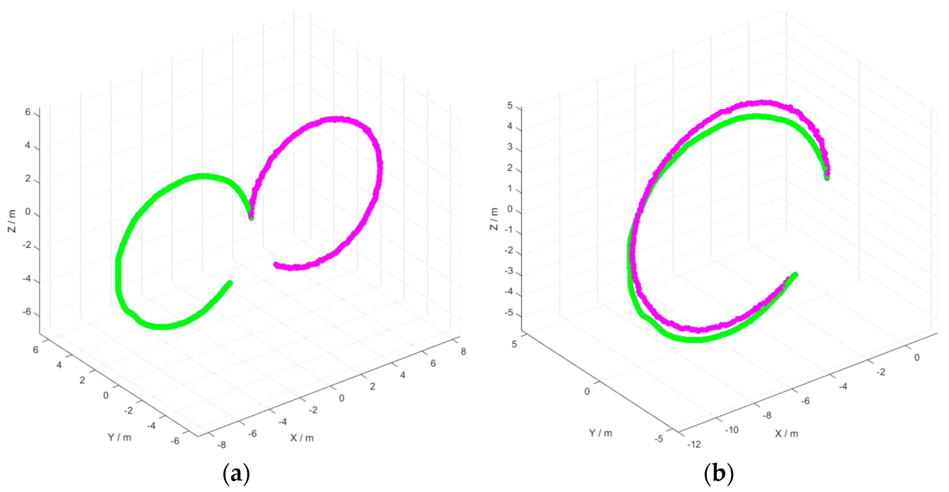
Figure 7 shows the alignment of the visual and the LiDAR motion trajectories. Specifically, Figure 7a depicts the original trajectories of the camera and LiDAR sensor, where pink indicates the LiDAR motion trajectory and green indicates the scale-recovered visual motion trajectory. Figure 7b shows the results of the aligned trajectories after the spatial transformation. It is evident that the two trajectories become more closely aligned after transformation, demonstrating that the calibration result obtained from the optimization iteration is fundamentally correct. This calibration result serves as the initial value for the next-stage calibration (referred to as the “initial value” below).

During the motion data collection, eight groups of synchronized point clouds and image data were randomly selected from the scene for refinement calibration. After 500 iterations, the final extrinsic parameters could be obtained (referred to as the “final value” below). The calibration results and root mean square errors are presented in

Table 1. Rotation calibration results of the simulation experiments.

	Rotation (°)			RMSE (°)
	Roll	Pitch	Yaw
Ground Truth	−90	0	−90	-
Initial Value	−88.120	−1.233	−90.323	1.311
Final Value	−89.818	0.058	−90.067	0.252

and

Table 2. Translation calibration results of simulation experiments.

	Translation (m)			RMSE (m)
	x	y	z
Ground Truth	−0.046	0.066	0	-
Initial Value	−0.088	0.117	−0.139	0.089
Final Value	−0.043	0.081	0.002	0.009

, respectively.

Table 1 and Table 2 present the preset reference truths, initial values, and final values for both the rotation and translation parts. The results show that the initial rotation values have a root mean square error of 1.311°, and the initial translation values have a root mean square error of 8.9 cm. Although the accuracy is relatively low, using these initial values to guide the subsequent optimization is sufficient. From the final calibration results, it is evident that the rotation achieves a root mean square error of 0.252°, and that of the translation is 0.9 cm. This demonstrates that accurate calibration results can be obtained using the proposed method.

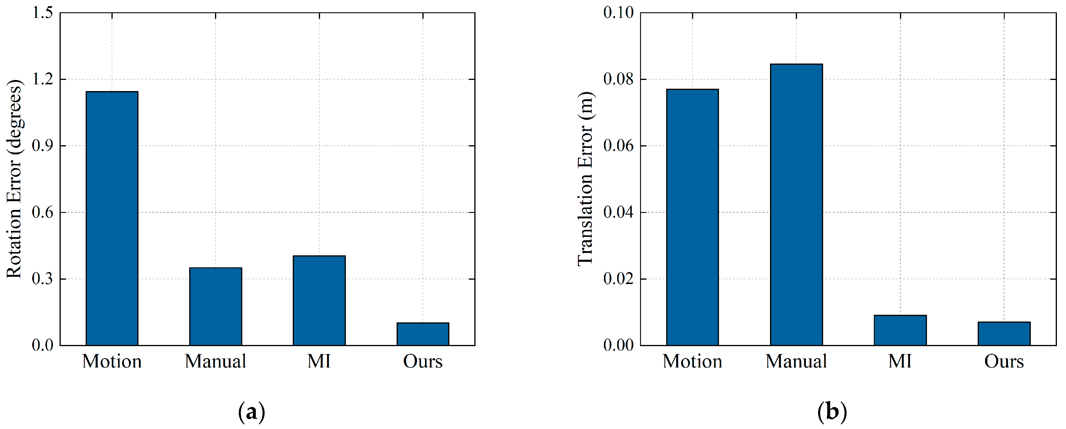
Based on our calibration results, we compared them with the results from motion-based [33], manual [47], and mutual-information methods [32], as shown in Figure 8. For the motion-based method, the data from the first stage of our method were used; for the manual method, 20 2D–3D correspondences were manually selected; and for the mutual-information method, eight groups of data from the second stage of the proposed method were used for statistical analysis. The results show that both the rotation and translation errors of the proposed method are lower than those of the other methods. In particular, on the same dataset, the proposed method demonstrates higher accuracy than the mutual-information method, validating the superiority of the proposed method in terms of accuracy.

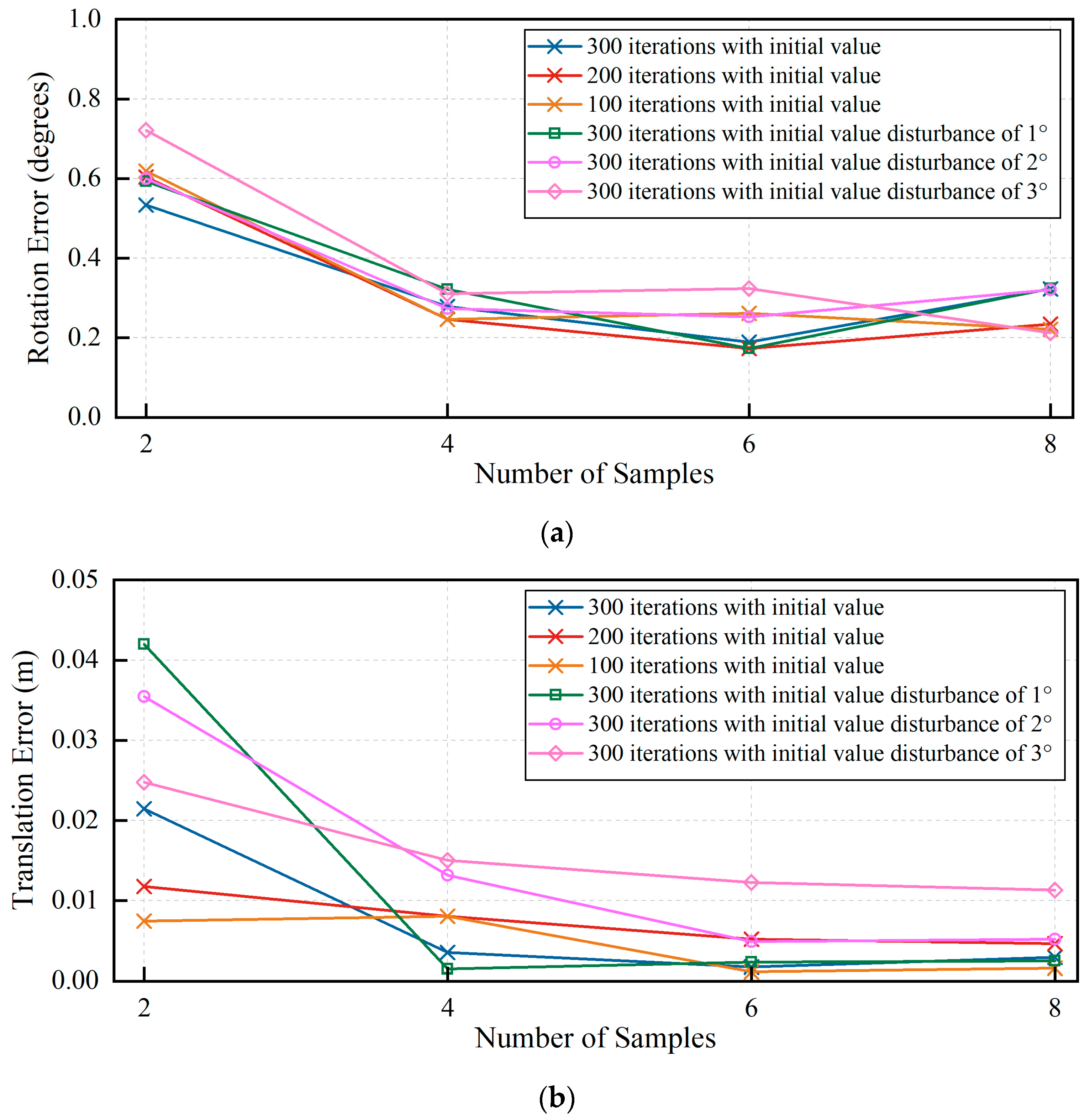
Once the initial extrinsic parameters were obtained, the refinement calibration was executed automatically. However, more data samples led to higher computational complexity, requiring a longer computational time. To validate the impact of sample size on the calibration accuracy in refinement calibration, we collected four groups of data of different sample sizes for the experiments. Different iteration numbers and disturbances were set to the initial values. The purpose was to explore the variation trends of the calibration results with different sample sizes, as well as the effects of different iteration numbers and initial values on the final accuracy.

The experimental results are shown in Figure 9. It is evident that when the sample size increases from two to four, both the rotation and translation errors decrease markedly until the sample size reaches eight, where the trend levels off. When the sample size is small, the disturbance effect of the initial values on the calibration accuracy is greater. As shown in Figure 9b, when the sample size is two, the mean absolute translation errors after the initial value disturbance range from 2 to 5 cm. However, when the sample size is greater than or equal to four, the effects of different iteration numbers and initial value disturbances on the final accuracy are limited. This indicates that the proposed calibration method demonstrates strong robustness.

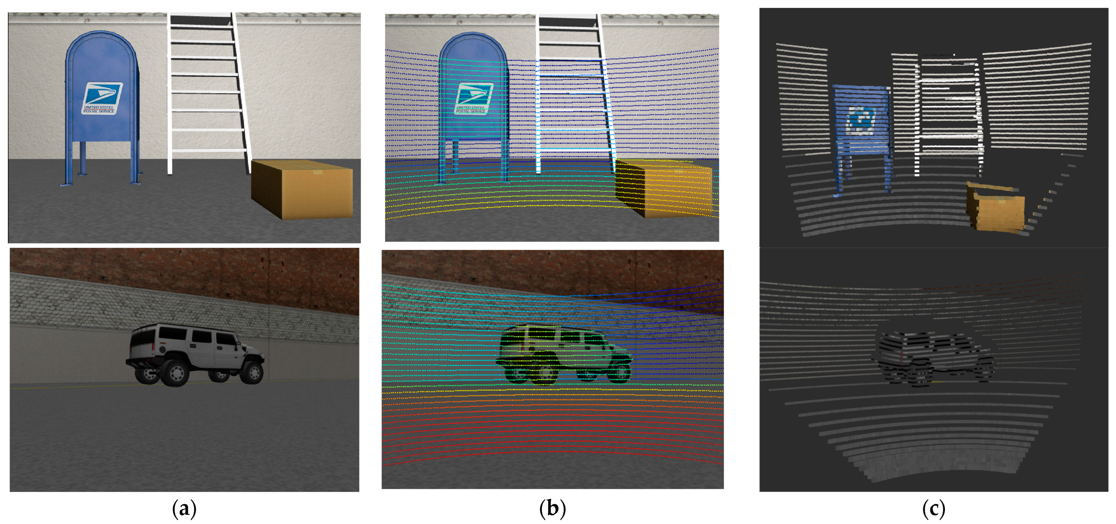
From a qualitative perspective, Figure 10 provides two types of visualization results. In Figure 10b, the point clouds at different distances are colored differently, making it easy to observe the alignment between the point clouds and objects. Figure 10c shows the fusion results of the point cloud and image using extrinsic parameters. The reliability of the calibration results can be determined by observing the RGB point clouds. Taken together, the visualization results shown in Figure 10 demonstrate the high quality of the extrinsic parameters between the camera and LiDAR sensor, further validating the accuracy of the proposed method.

5.3. Real Experiment

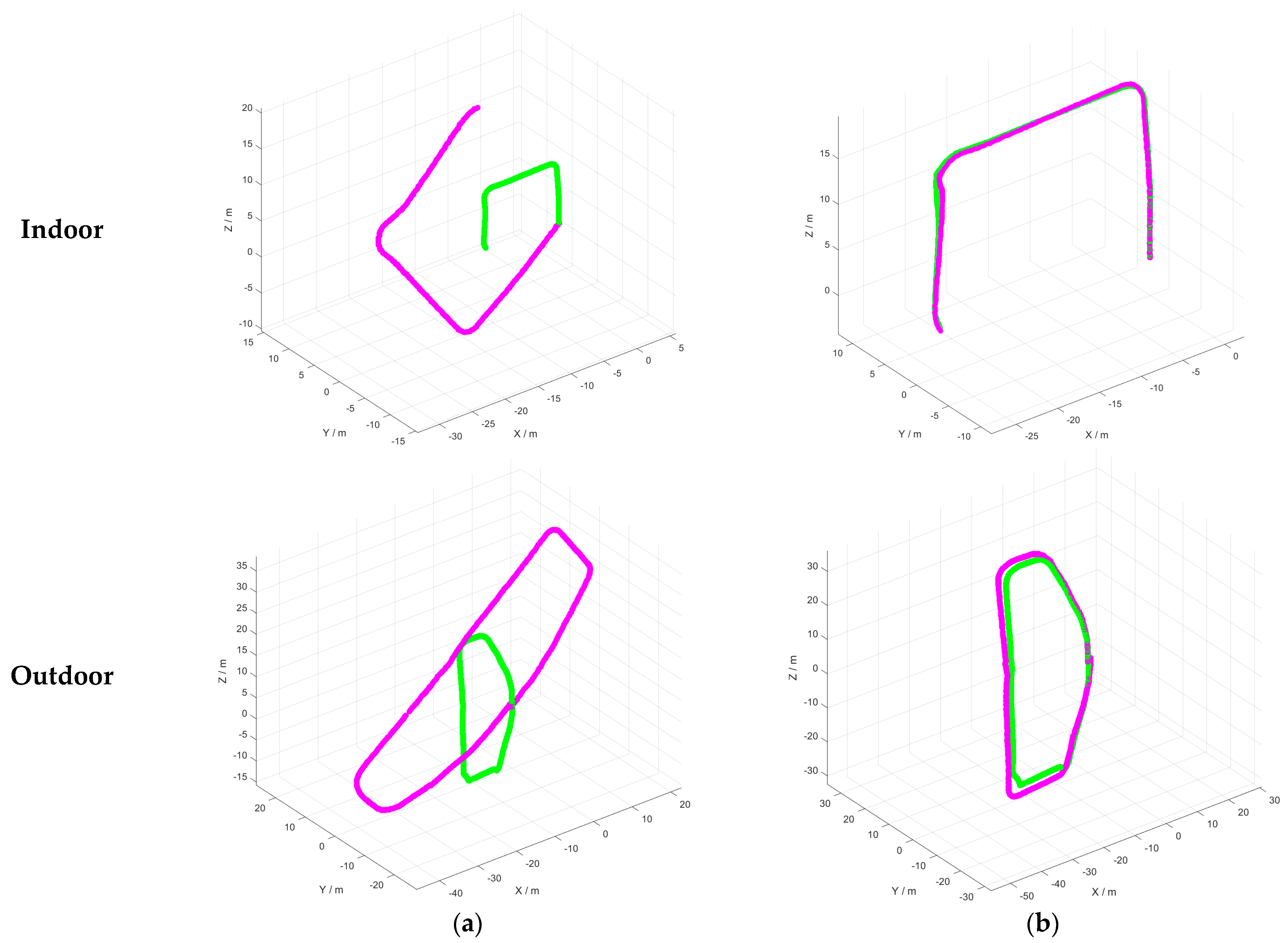
In real-world experiments, we tested different environments. In the initial extrinsic calibration process, we collected 1400 and 3000 frames of pose data indoors and outdoors, respectively, and performed 30 optimization iterations to solve the parameters. The optimization results are shown in Figure 11, where green depicts the scaled visual trajectory and pink depicts the LiDAR trajectory. Figure 11a shows the original trajectories of the camera and LiDAR sensor. There was a scale difference between visual trajectory and LiDAR trajectory, which can be attributed to the scale uncertainty of monocular visual odometry. Through continuous iterations, the two trajectories gradually converge, the final result being as shown in Figure 11b. The optimization results demonstrate that both calibrations are correct and reliable and can serve as initial external parameters for the refinement calibration stage.

In the refinement calibration stage, based on experience from the simulation experiments, we randomly collected four, six, and eight samples of data indoors and outdoors, respectively. After 200 iterations, the final calibration parameters were obtained, the final calibration results being as listed in

Table 3. Calibration results from real experiments.

Scene	Samples	Roll (°)	Pitch (°)	Yaw (°)	x (m)	y (m)	z (m)
Indoor	N = 4	−89.204	−0.561	139.049	0.022	−0.096	−0.153
	N = 6	−89.188	−0.693	139.130	0.020	−0.057	−0.174
	N = 8	−89.118	−0.775	139.316	0.010	−0.054	−0.196
Outdoor	N = 4	−88.893	−0.389	139.037	0.022	−0.088	−0.183
	N = 6	−88.793	−0.714	139.274	0.020	−0.053	−0.175
	N = 8	−88.981	−0.505	139.316	0.021	−0.056	−0.162

. As verified by the simulation experiments, when the number of samples is greater than or equal to four, the calibration results tend to stabilize for both scenarios. The rotation calibration results differ by no more than 0.4°, and the translation calibration results differ by less than 5 cm, demonstrating the excellent performance of the experiments indoors and outdoors. The standard deviation results shown in

Table 4. Standard deviations of calibration results.

Scene	Rotation Standard Deviation (°)	Translation Standard Deviation (m)
Indoor	0.060	0.011
Outdoor	0.080	0.007

demonstrate small fluctuations in the calibration outcomes, further validating the stability of the calibration system.

As the true extrinsic parameters of the camera and LiDAR sensor were unknown, the specific calibration accuracy could not be calculated. Instead, the relative differences were compared by visualizing the calibration results. In this study, a point cloud was projected onto an image plane using the average of the calibration results to visually judge the accuracy of the extrinsic parameters. Figure 12 shows the projection results for three different scenarios compared to the motion-based [33], manual [47], and mutual-information-based methods [32]. As seen in the red boxes in Figure 12, compared with the other methods, the correspondence between the LiDAR point cloud and the image is better for the proposed method as the projected LiDAR points are closer to the image edges.

6. Discussion

The initial calibration stage used the hand–eye calibration model. When aligning the motion of the camera and LiDAR sensor, owing to differences in the odometry extraction accuracy and data collection synchronization deviations between different sensors, these deviations are propagated into extrinsic calibration errors, noise and error accumulation being the main causes of deviations in odometry accuracy. In particular, the scale ambiguity of monocular visual odometry results in an inability to determine the precise scale relationship between the camera and LiDAR sensor, even if the scale is optimized. The initial values exhibit an unsatisfactory calibration accuracy (Table 1 and Table 2).

Consequently, in the refinement calibration, we used the edge information in the scene to improve the calibration accuracy. The initial extrinsic parameters obtained from the initial calibration reduce the search space in the subsequent refinement calibration, thus lowering the calibration difficulty and improving efficiency. This coarse-to-fine calibration strategy is effective because it makes full use of prior information and diverse features by decomposing the calibration into two subproblems. Refinement calibration considers the initial calibration results as a starting point, which effectively reduces error propagation and accumulation, resulting in a more accurate calibration. The final errors listed in Table 1 and Table 2 confirm this.

As shown in Figure 8, compared to the other targetless methods, the proposed calibration method achieves the smallest errors. Manual calibration requires tedious manual operations to be introduced, making the calibration more subjective and complex. The mutual-information method estimates the extrinsic parameters by calculating the correlation between the grayscale image and point-cloud reflectance using kernel density estimation, maximizing this correlation. This method can be susceptible to environmental illumination and material reflectance, but the influence of environmental factors can be minimized by fixing the focus and exposure. Consequently, it can achieve good calibration accuracy in most environments.

During the experiments, although the proposed method exhibited superiority in various scenarios, some challenges remain under extreme conditions, such as low textures and complex environments. Once the edge features become difficult to identify or redundant, multiple local optima tend to appear, causing the calibration to fall into local optimum traps, making it necessary to improve the initial calibration accuracy to reduce the search space complexity. Similarly, selecting features from specific objects as the algorithm input can be challenging.

7. Conclusions

A camera–LiDAR extrinsic calibration method based on motion and edge matching was proposed. Unlike most existing solutions, this system could be calibrated without any initial estimation of the sensor configuration. Additionally, the proposed method did not require markers or other calibration aids. This process comprised two stages. First, the motion poses of the camera and LiDAR sensor were estimated using visual and LiDAR odometry techniques, and the resulting motion poses were interpolated. Furthermore, a hand–eye calibration model was applied to solve the extrinsic parameters, whose results served as the initial values for the next stage of calibration. Subsequently, by aligning the edge information in the co-observed scenes, the initial extrinsic parameters were further optimized to improve the final calibration accuracy.

The performance of the system was verified through a series of simulations and real-world experiments. Experimental evaluations validated the proposed method, demonstrating its ability to achieve precise calibration without manual initialization or external calibration aids. Compared to other targetless calibration methods, the proposed method achieved higher calibration accuracy.

However, several issues remain to be addressed in future studies:

• Although we achieved calibration in various scenes—such as indoor and outdoor scenes—feature loss still exists in high-speed motion and weak-texture scenes. Deeper data mining is the focus of future research.
• Extracting useful semantic edges using deep-learning methods could be a solution to reduce the complexity of optimization [48]. This methodology offers novel insights that can effectively overcome the limitations encountered in specific calibration scenarios.
• The extrinsic calibration between the camera and LiDAR sensor is the basis for higher-level fusion between the two sensors. However, more algorithms are required to realize feature- and decision-level fusion. We intend to further investigate the field of multi-sensor fusion technology through our ongoing research efforts.