
Seasonal Effect of the Vegetation Clumping Index on Gross Primary Productivity Estimated by a Two-Leaf Light Use Efficiency Model


 , ,
, ,
Abstract
:1. Introduction
2. Data
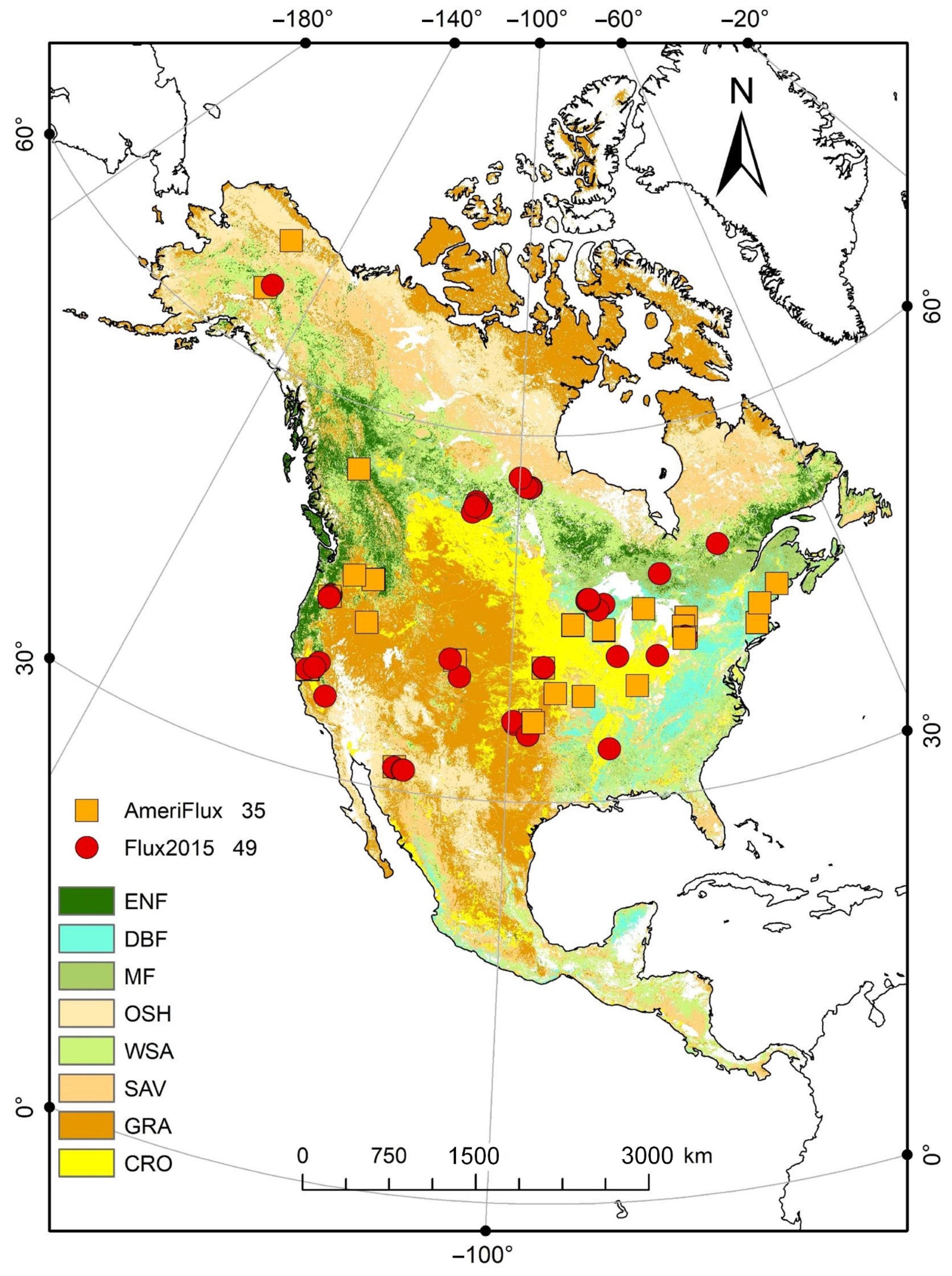
2.1. Flux Site Data
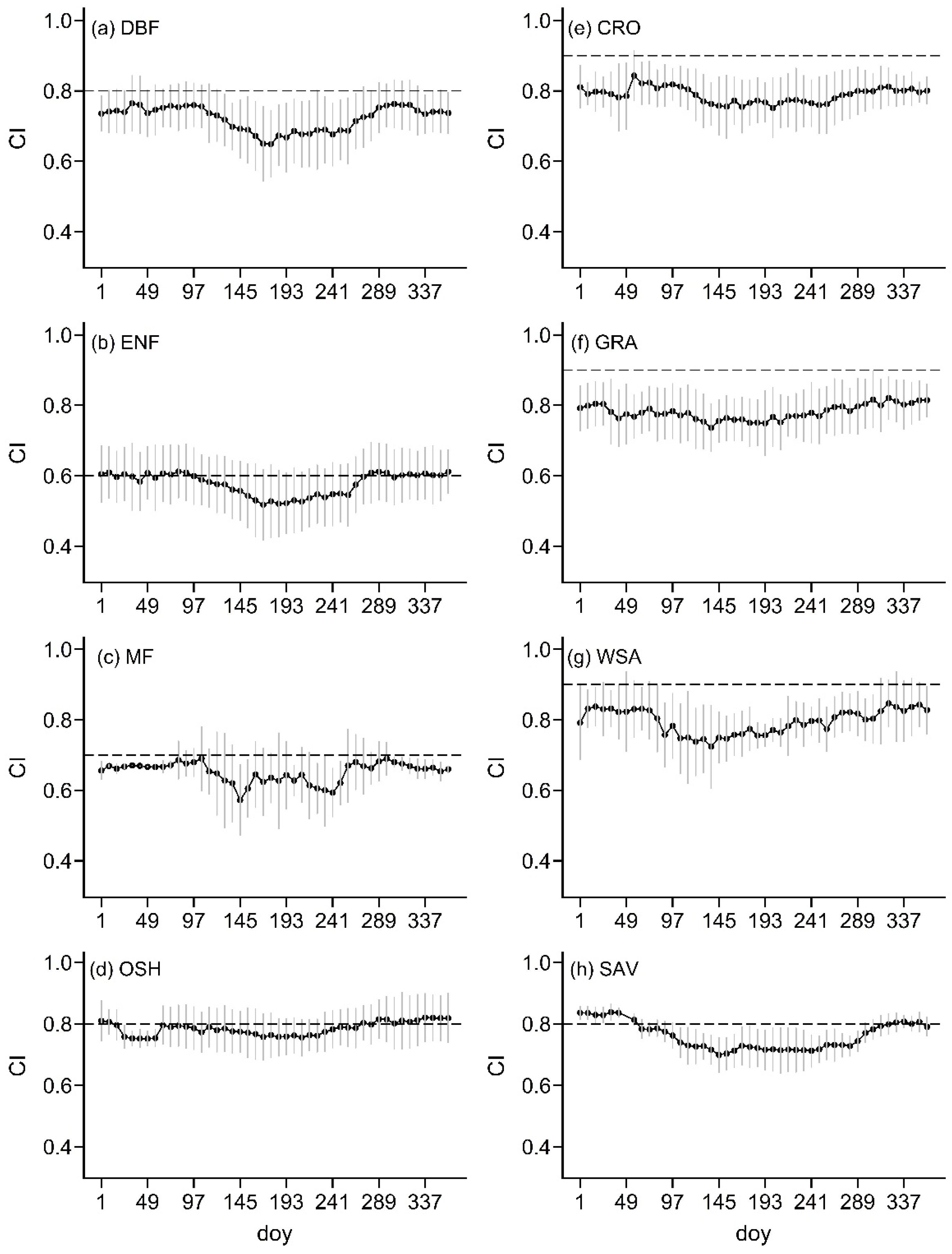
2.2. MODIS CI
2.3. MODIS Land Cover and LAI
2.4. Meteorological Data
3. Model and Methods
3.1. Two-Leaf Light Use Efficiency Model
3.2. Sensitivity Analysis by SIMLAB
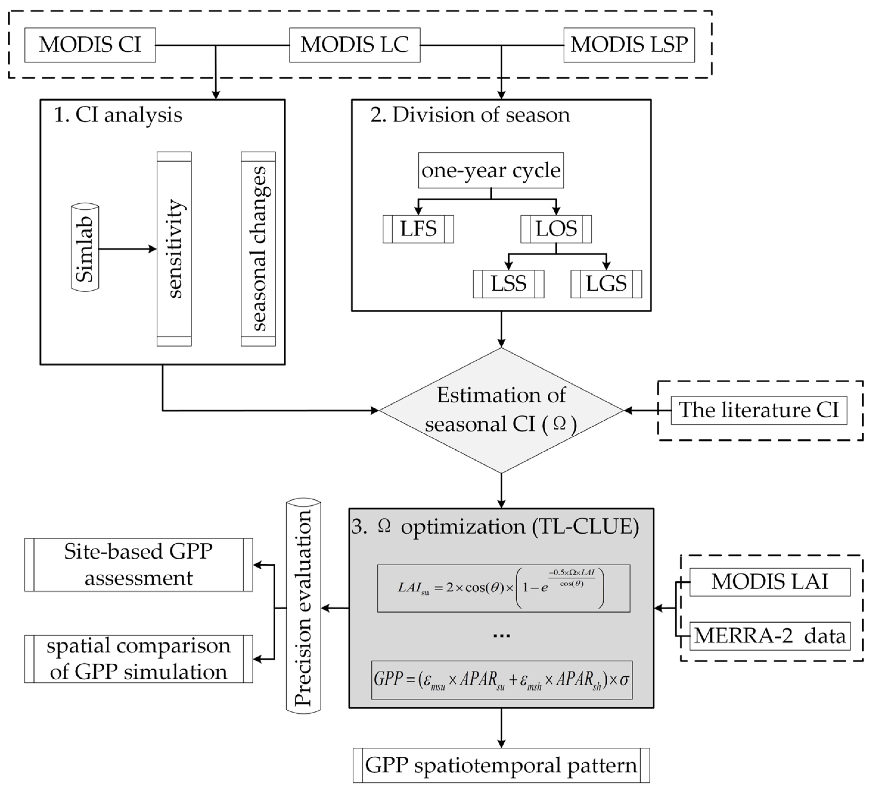
3.3. Description of the TL-CLUE Model
3.4. Model Evaluation Metrics
4. Results
4.1. Changes in GPP and CI in Different Vegetation Types
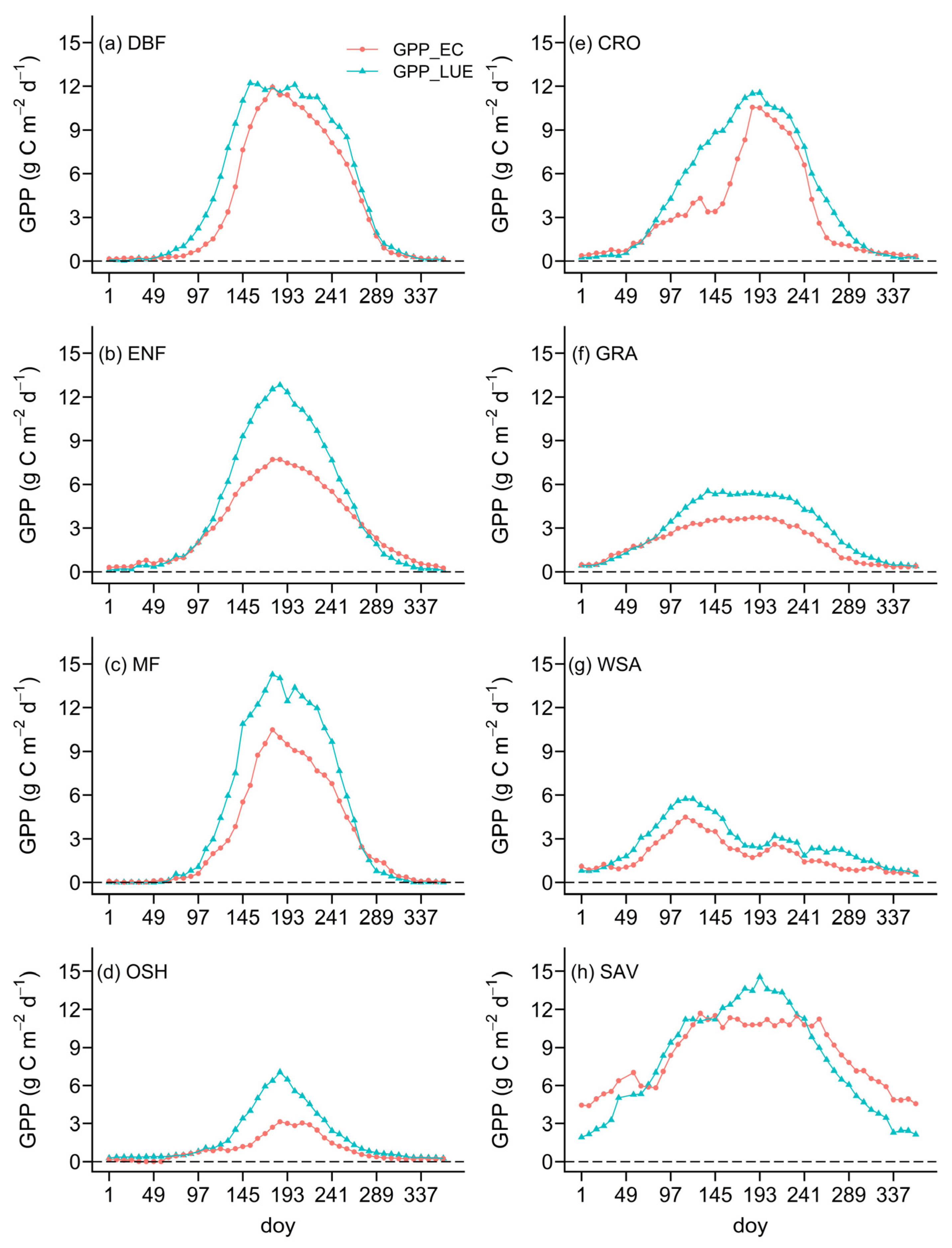
4.1.1. Eight-Day Changes in GPP
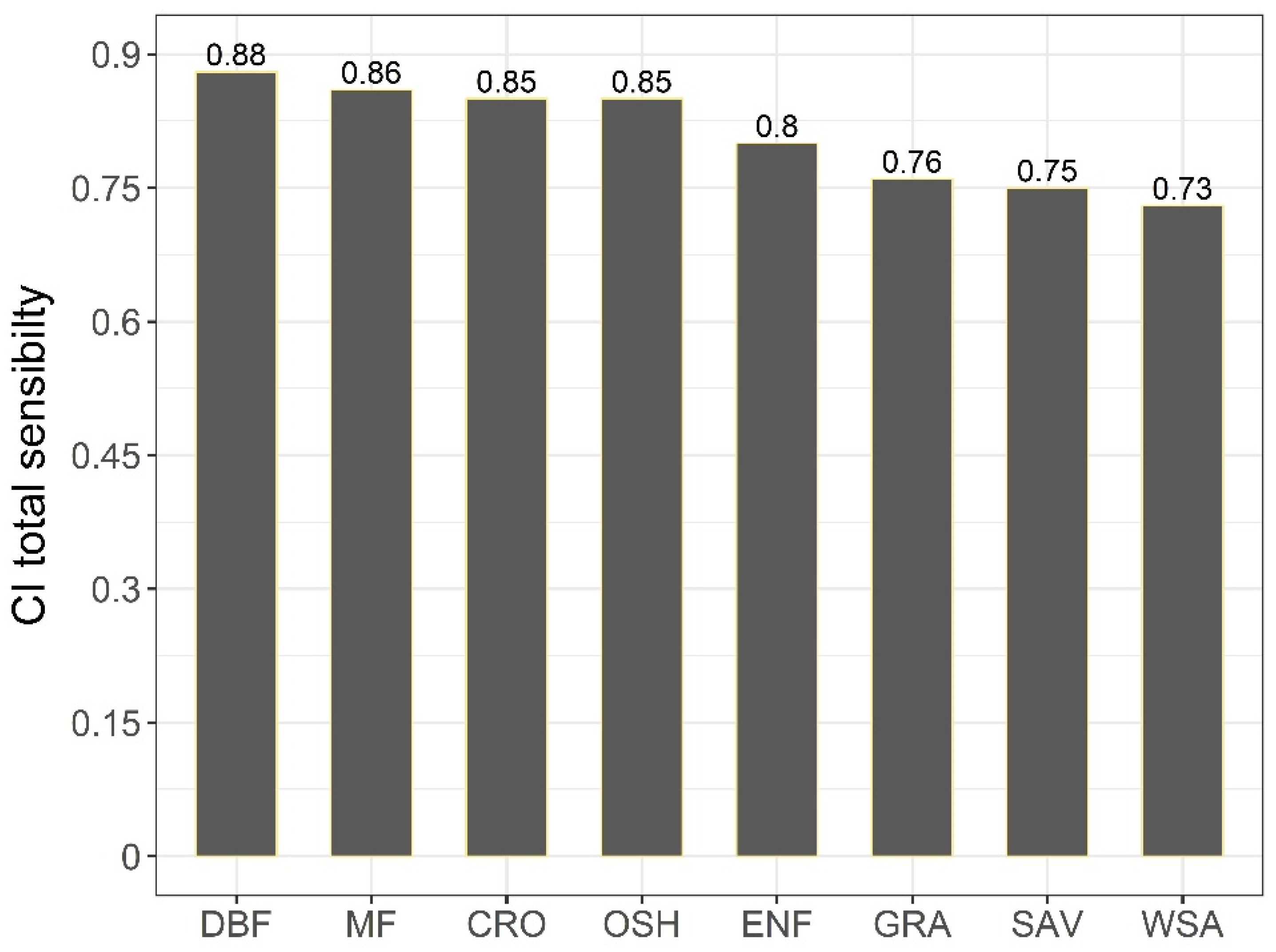
4.1.2. Sensitivity of GPP to CI of Different Vegetation Types
4.2. Evaluation of GPP Estimated by the TL-CLUE Model
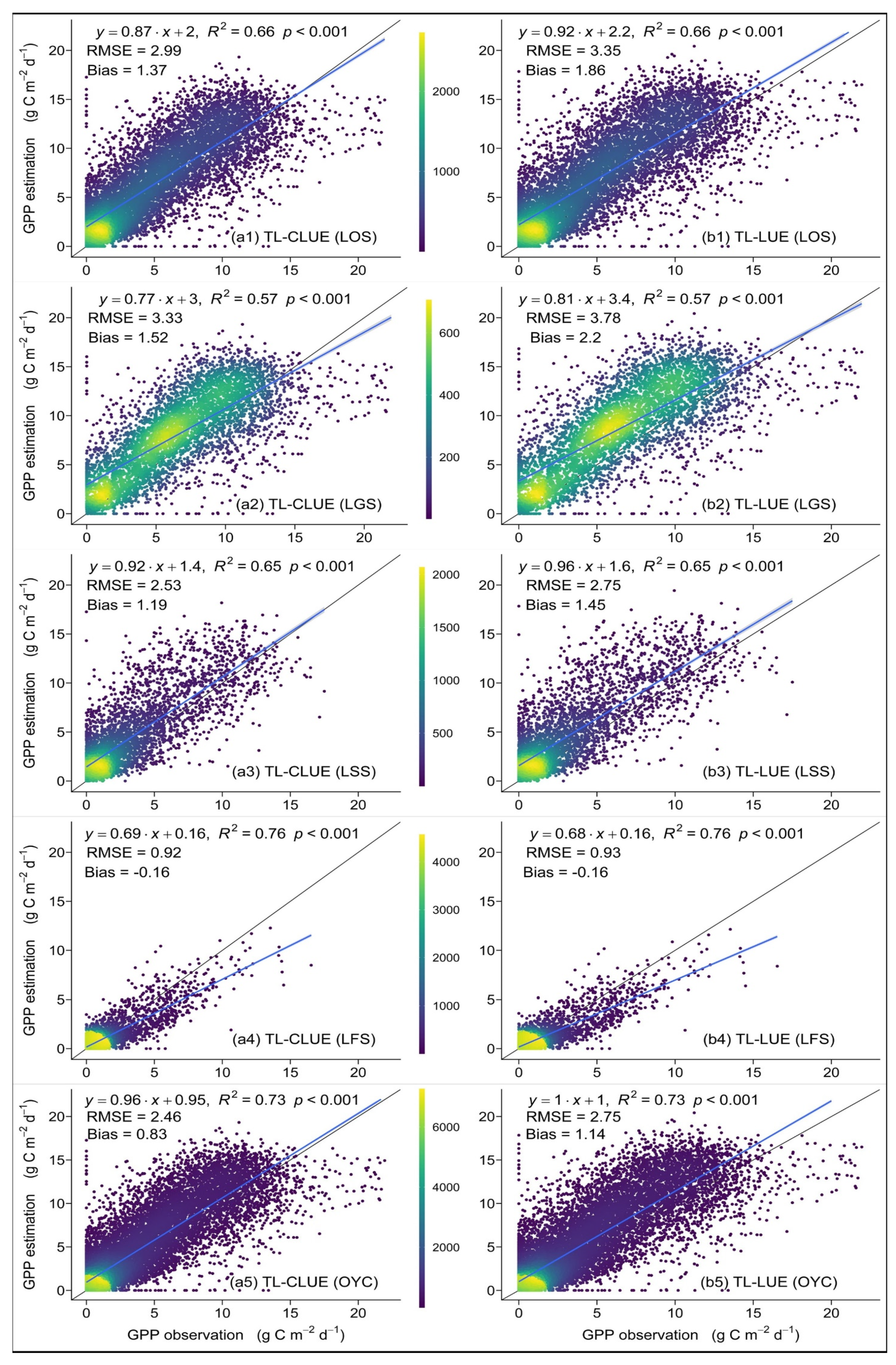
4.2.1. Verification of GPP Estimation against Sites
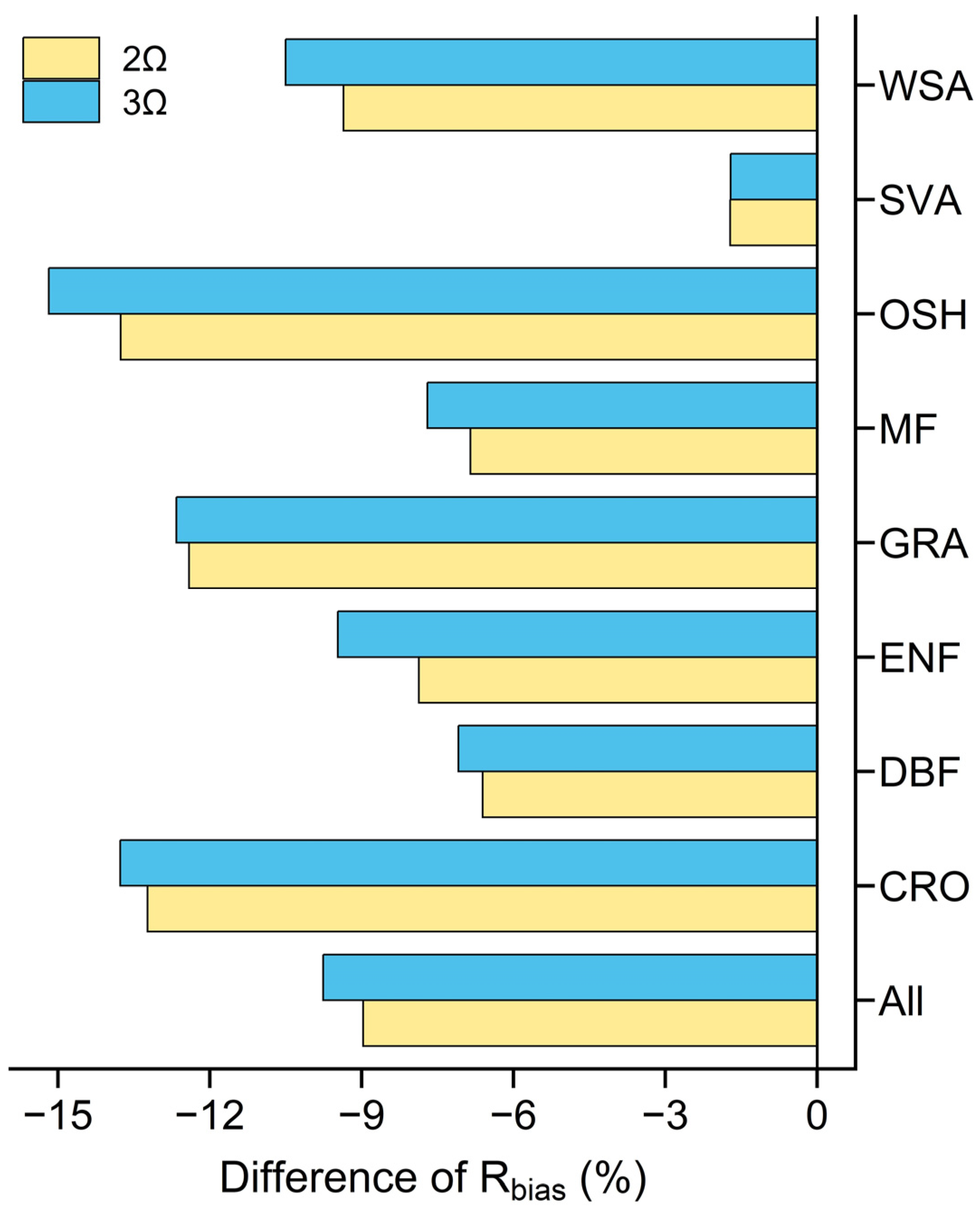
4.2.2. Accuracy of GPP Estimation under Three and Two Estimations of CI
4.3. Spatial and Temporal Patterns of GPP across North America
4.3.1. GPP Difference between the TL-CLUE and TL-LUE Models
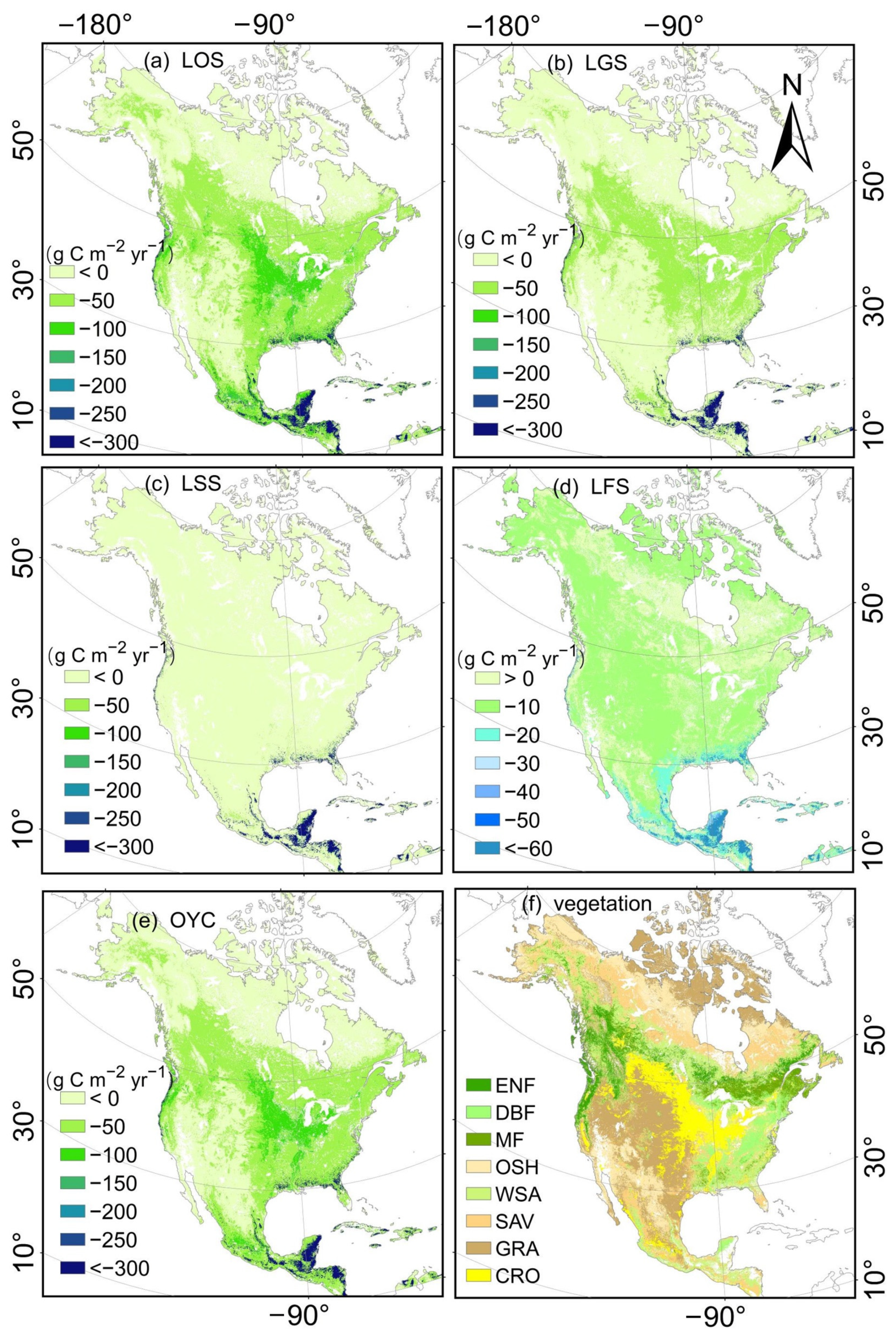
4.3.2. Spatial Characteristics of Seasonal GPP Simulation in the TL-CLUE Model
5. Discussion
6. Conclusions
Author Contributions
Funding
Data Availability Statement
Acknowledgments
Conflicts of Interest
References
- Chapin, F.S.; Matson, P.A.; Mooney, H.A.; Vitousek, P.M. Principles of Terrestrial Ecosystem Ecology; Springer: New York, NY, USA, 2002; pp. 3–22. ISBN 978-971-4419-9504-4419. [Google Scholar]
- Friedlingstein, P.; Jones, M.W.; O’sullivan, M.; Andrew, R.M.; Hauck, J.; Peters, G.P.; Peters, W.; Pongratz, J.; Sitch, S.; Le Quéré, C. Global carbon budget 2019. Earth Syst. Sci. Data 2019, 11, 1783–1838. [Google Scholar] [CrossRef]
- Beer, C.; Reichstein, M.; Tomelleri, E.; Ciais, P.; Jung, M.; Carvalhais, N.; Rödenbeck, C.; Arain, M.A.; Baldocchi, D.; Bonan, G.B. Terrestrial gross carbon dioxide uptake: Global distribution and covariation with climate. Science 2010, 329, 834–838. [Google Scholar] [CrossRef]
- He, M.; Ju, W.; Zhou, Y.; Chen, J.; He, H.; Wang, S.; Wang, H.; Guan, D.; Yan, J.; Li, Y. Development of a two-leaf light use efficiency model for improving the calculation of terrestrial gross primary productivity. Agric. For. Meteorol. 2013, 173, 28–39. [Google Scholar] [CrossRef]
- Hilton, T.W.; Whelan, M.E.; Zumkehr, A.; Kulkarni, S.; Berry, J.A.; Baker, I.T.; Montzka, S.A.; Sweeney, C.; Miller, B.R.; Elliott Campbell, J. Peak growing season gross uptake of carbon in North America is largest in the Midwest USA. Nat. Clim. Chang. 2017, 7, 450–454. [Google Scholar] [CrossRef]
- Chang, J.; Ciais, P.; Wang, X.; Piao, S.; Asrar, G.; Betts, R.; Chevallier, F.; Dury, M.; François, L.; Frieler, K. Benchmarking carbon fluxes of the ISIMIP2a biome models. Environ. Res. Lett. 2017, 12, 045002. [Google Scholar] [CrossRef]
- Ito, A.; Nishina, K.; Reyer, C.P.; François, L.; Henrot, A.-J.; Munhoven, G.; Jacquemin, I.; Tian, H.; Yang, J.; Pan, S. Photosynthetic productivity and its efficiencies in ISIMIP2a biome models: Benchmarking for impact assessment studies. Environ. Res. Lett. 2017, 12, 085001. [Google Scholar] [CrossRef]
- Monteith, J.L. Solar radiation and productivity in tropical ecosystems. J. Appl. Ecol. 1972, 9, 747–766. [Google Scholar] [CrossRef]
- Potter, C.S.; Randerson, J.T.; Field, C.B.; Matson, P.A.; Vitousek, P.M.; Mooney, H.A.; Klooster, S.A. Terrestrial ecosystem production: A process model based on global satellite and surface data. Glob. Biogeochem. Cycles 1993, 7, 811–841. [Google Scholar] [CrossRef]
- Xiao, X.; Hollinger, D.; Aber, J.; Goltz, M.; Davidson, E.A.; Zhang, Q.; Moore III, B. Satellite-based modeling of gross primary production in an evergreen needleleaf forest. Remote Sens. Environ. 2004, 89, 519–534. [Google Scholar] [CrossRef]
- Guan, X.; Chen, J.M.; Shen, H.; Xie, X. A modified two-leaf light use efficiency model for improving the simulation of GPP using a radiation scalar. Agric. For. Meteorol. 2021, 307, 108546. [Google Scholar] [CrossRef]
- Zheng, Y.; Shen, R.; Wang, Y.; Li, X.; Liu, S.; Liang, S.; Chen, J.M.; Ju, W.; Zhang, L.; Yuan, W. Improved estimate of global gross primary production for reproducing its long-term variation, 1982–2017. Earth Syst. Sci. Data 2020, 12, 2725–2746. [Google Scholar] [CrossRef]
- Marshall, M.; Tu, K.; Brown, J. Optimizing a remote sensing production efficiency model for macro-scale GPP and yield estimation in agroecosystems. Remote Sens. Environ. 2018, 217, 258–271. [Google Scholar] [CrossRef]
- Guan, X.; Shen, H.; Li, X.; Gan, W.; Zhang, L. A long-term and comprehensive assessment of the urbanization-induced impacts on vegetation net primary productivity. Sci. Total Environ. 2019, 669, 342–352. [Google Scholar] [CrossRef]
- Zhang, Y.; Xiao, X.; Wu, X.; Zhou, S.; Zhang, G.; Qin, Y.; Dong, J. A global moderate resolution dataset of gross primary production of vegetation for 2000–2016. Sci. Data 2017, 4, 1–13. [Google Scholar] [CrossRef] [PubMed]
- Running, S.W.; Nemani, R.; Glassy, J.M.; Thornton, P.E. MODIS Daily Photosynthesis (PSN) and Annual Net Primary Production (NPP) Product (MOD17) Algorithm Theoretical Basis Document; NASA Goddard Space Flight Cent.: Greenbelt, MD, USA, 1999.
- Dong, J.; Xiao, X.; Wagle, P.; Zhang, G.; Zhou, Y.; Jin, C.; Torn, M.S.; Meyers, T.P.; Suyker, A.E.; Wang, J. Comparison of four EVI-based models for estimating gross primary production of maize and soybean croplands and tallgrass prairie under severe drought. Remote Sens. Environ. 2015, 162, 154–168. [Google Scholar] [CrossRef]
- Yuan, W.; Zheng, Y.; Piao, S.; Ciais, P.; Lombardozzi, D.; Wang, Y.; Ryu, Y.; Chen, G.; Dong, W.; Hu, Z. Increased atmospheric vapor pressure deficit reduces global vegetation growth. Sci. Adv. 2019, 5, eaax1396. [Google Scholar] [CrossRef] [PubMed]
- Zhao, M.; Running, S.W. Drought-induced reduction in global terrestrial net primary production from 2000 through 2009. Science 2010, 329, 940–943. [Google Scholar] [CrossRef] [PubMed]
- Zhang, Y.; Song, C.; Sun, G.; Band, L.E.; Noormets, A.; Zhang, Q. Understanding moisture stress on light use efficiency across terrestrial ecosystems based on global flux and remote-sensing data. J. Geophys. Res. Biogeosci. 2015, 120, 2053–2066. [Google Scholar] [CrossRef]
- Sun, Z.; Wang, X.; Zhang, X.; Tani, H.; Guo, E.; Yin, S.; Zhang, T. Evaluating and comparing remote sensing terrestrial GPP models for their response to climate variability and CO2 trends. Sci. Total Environ. 2019, 668, 696–713. [Google Scholar] [CrossRef]
- Mäkelä, A.; Pulkkinen, M.; Kolari, P.; Lagergren, F.; Berbigier, P.; Lindroth, A.; Loustau, D.; Nikinmaa, E.; Vesala, T.; Hari, P. Developing an empirical model of stand GPP with the LUE approach: Analysis of eddy covariance data at five contrasting conifer sites in Europe. Glob. Chang. Biol. 2008, 14, 92–108. [Google Scholar] [CrossRef]
- Yu, R. An improved estimation of net primary productivity of grassland in the Qinghai-Tibet region using light use efficiency with vegetation photosynthesis model. Ecol. Modell. 2020, 431, 109121. [Google Scholar] [CrossRef]
- Wang, H.; Jia, G.; Fu, C.; Feng, J.; Zhao, T.; Ma, Z. Deriving maximal light use efficiency from coordinated flux measurements and satellite data for regional gross primary production modeling. Remote Sens. Environ. 2010, 114, 2248–2258. [Google Scholar] [CrossRef]
- Yuan, W.; Liu, S.; Zhou, G.; Zhou, G.; Tieszen, L.L.; Baldocchi, D.; Bernhofer, C.; Gholz, H.; Goldstein, A.H.; Goulden, M.L. Deriving a light use efficiency model from eddy covariance flux data for predicting daily gross primary production across biomes. Agric. For. Meteorol. 2007, 143, 189–207. [Google Scholar] [CrossRef]
- Monteith, J.L. Climate and the efficiency of crop production in Britain. Phil. Trans. R. Soc. Lond. B 1977, 281, 277–294. [Google Scholar] [CrossRef]
- Wang, Y.-P.; Leuning, R. A two-leaf model for canopy conductance, photosynthesis and partitioning of available energy I:: Model description and comparison with a multi-layered model. Agric. For. Meteorol. 1998, 91, 89–111. [Google Scholar] [CrossRef]
- Propastin, P.; Ibrom, A.; Knohl, A.; Erasmi, S. Effects of canopy photosynthesis saturation on the estimation of gross primary productivity from MODIS data in a tropical forest. Remote Sens. Environ. 2012, 121, 252–260. [Google Scholar] [CrossRef]
- Chen, J.; Liu, J.; Cihlar, J.; Goulden, M. Daily canopy photosynthesis model through temporal and spatial scaling for remote sensing applications. Ecol. Modell. 1999, 124, 99–119. [Google Scholar] [CrossRef]
- De Pury, D.; Farquhar, G. Simple scaling of photosynthesis from leaves to canopies without the errors of big-leaf models. Plant Cell Environ. 1997, 20, 537–557. [Google Scholar] [CrossRef]
- Rap, A.; Scott, C.; Reddington, C.; Mercado, L.; Ellis, R.; Garraway, S.; Evans, M.; Beerling, D.; MacKenzie, A.; Hewitt, C. Enhanced global primary production by biogenic aerosol via diffuse radiation fertilization. Nat. Geosci. 2018, 11, 640–644. [Google Scholar] [CrossRef]
- He, L.; Liu, J.; Chen, J.M.; Croft, H.; Wang, R.; Sprintsin, M.; Zheng, T.; Ryu, Y.; Pisek, J.; Gonsamo, A. Inter-and intra-annual variations of clumping index derived from the MODIS BRDF product. Int. J. Appl. Earth Obs. Geoinf. 2016, 44, 53–60. [Google Scholar] [CrossRef]
- Chen, B.; Arain, M.A.; Chen, J.M.; Wang, S.; Fang, H.; Liu, Z.; Mo, G.; Liu, J. Importance of shaded leaf contribution to the total GPP of Canadian terrestrial ecosystems: Evaluation of MODIS GPP. J. Geophys. Res. Biogeosci. 2020, 125, e2020JG005917. [Google Scholar] [CrossRef]
- Cheng, S.J.; Bohrer, G.; Steiner, A.L.; Hollinger, D.Y.; Suyker, A.; Phillips, R.P.; Nadelhoffer, K.J. Variations in the influence of diffuse light on gross primary productivity in temperate ecosystems. Agric. For. Meteorol. 2015, 201, 98–110. [Google Scholar] [CrossRef]
- Zhang, M.; Yu, G.-R.; Zhuang, J.; Gentry, R.; Fu, Y.-L.; Sun, X.-M.; Zhang, L.-M.; Wen, X.-F.; Wang, Q.-F.; Han, S.-J. Effects of cloudiness change on net ecosystem exchange, light use efficiency, and water use efficiency in typical ecosystems of China. Agric. For. Meteorol. 2011, 151, 803–816. [Google Scholar] [CrossRef]
- Zhou, Y.; Wu, X.; Ju, W.; Chen, J.M.; Wang, S.; Wang, H.; Yuan, W.; Andrew Black, T.; Jassal, R.; Ibrom, A. Global parameterization and validation of a two-leaf light use efficiency model for predicting gross primary production across FLUXNET sites. Geophys. Res. Biogeosci. 2016, 121, 1045–1072. [Google Scholar] [CrossRef]
- Nilson, T. A theoretical analysis of the frequency of gaps in plant stands. Agric. Meteorol. 1971, 8, 25–38. [Google Scholar] [CrossRef]
- Govind, A.; Guyon, D.; Roujean, J.-L.; Yauschew-Raguenes, N.; Kumari, J.; Pisek, J.; Wigneron, J.-P. Effects of canopy architectural parameterizations on the modeling of radiative transfer mechanism. Ecol. Model. 2013, 251, 114–126. [Google Scholar] [CrossRef]
- Chen, B.; Coops, N.C.; Fu, D.; Margolis, H.A.; Amiro, B.D.; Black, T.A.; Arain, M.A.; Barr, A.G.; Bourque, C.P.-A.; Flanagan, L.B. Characterizing spatial representativeness of flux tower eddy-covariance measurements across the Canadian Carbon Program Network using remote sensing and footprint analysis. Remote Sens. Environ. 2012, 124, 742–755. [Google Scholar] [CrossRef]
- Chen, H.; Niu, Z.; Huang, W.; Feng, J. Predicting leaf area index in wheat using an improved empirical model. J. Appl. Remote Sens. 2013, 7, 073577. [Google Scholar] [CrossRef]
- Mercado, L.; Lloyd, J.; Carswell, F.; Malhi, Y.; Meir, P.; Nobre, A.D. Modelling Amazonian forest eddy covariance data: A comparison of big leaf versus sun/shade models for the C-14 tower at Manaus I. Canopy photosynthesis. Acta Amaz. 2006, 36, 69–82. [Google Scholar] [CrossRef]
- Yin, S.; Jiao, Z.; Dong, Y.; Zhang, X.; Cui, L.; Xie, R.; Guo, J.; Li, S.; Zhu, Z.; Tong, Y. Evaluation of the Consistency of the Vegetation Clumping Index Retrieved from Updated MODIS BRDF Data. Remote Sens. 2022, 14, 3997. [Google Scholar] [CrossRef]
- Wei, S.; Fang, H.; Schaaf, C.B.; He, L.; Chen, J.M. Global 500 m clumping index product derived from MODIS BRDF data (2001–2017). Remote Sens. Environ. 2019, 232, 111296. [Google Scholar] [CrossRef]
- Pastorello, G.; Trotta, C.; Canfora, E.; Chu, H.; Christianson, D.; Cheah, Y.-W.; Poindexter, C.; Chen, J.; Elbashandy, A.; Humphrey, M. The FLUXNET2015 dataset and the ONEFlux processing pipeline for eddy covariance data. Sci. Data 2020, 7, 225. [Google Scholar] [CrossRef] [PubMed]
- Reichstein, M.; Falge, E.; Baldocchi, D.; Papale, D.; Aubinet, M.; Berbigier, P.; Bernhofer, C.; Buchmann, N.; Gilmanov, T.; Granier, A. On the separation of net ecosystem exchange into assimilation and ecosystem respiration: Review and improved algorithm. Glob. Chang. Biol. 2005, 11, 1424–1439. [Google Scholar] [CrossRef]
- Tang, S.; Chen, J.; Zhu, Q.; Li, X.; Chen, M.; Sun, R.; Zhou, Y.; Deng, F.; Xie, D. LAI inversion algorithm based on directional reflectance kernels. J. Environ. Manag. 2007, 85, 638–648. [Google Scholar] [CrossRef] [PubMed]
- Jiao, Z.; Dong, Y.; Schaaf, C.B.; Chen, J.M.; Román, M.; Wang, Z.; Zhang, H.; Ding, A.; Erb, A.; Hill, M.J. An algorithm for the retrieval of the clumping index (CI) from the MODIS BRDF product using an adjusted version of the kernel-driven BRDF model. Remote Sens. Environ. 2018, 209, 594–611. [Google Scholar] [CrossRef]
- Jiao, Z.; Schaaf, C.B.; Dong, Y.; Román, M.; Hill, M.J.; Chen, J.M.; Wang, Z.; Zhang, H.; Saenz, E.; Poudyal, R. A method for improving hotspot directional signatures in BRDF models used for MODIS. Remote Sens. Environ. 2016, 186, 135–151. [Google Scholar] [CrossRef]
- Savitzky, A.; Golay, M.J. Smoothing and differentiation of data by simplified least squares procedures. Anal. Chem. 1964, 36, 1627–1639. [Google Scholar] [CrossRef]
- Schmid, H. Experimental design for flux measurements: Matching scales of observations and fluxes. Agric. For. Meteorol. 1997, 87, 179–200. [Google Scholar] [CrossRef]
- Li, F.; Hao, D.; Zhu, Q.; Yuan, K.; Braghiere, R.K.; He, L.; Luo, X.; Wei, S.; Riley, W.J.; Zeng, Y. Vegetation clumping modulates global photosynthesis through adjusting canopy light environment. Glob. Chang. Biol. 2023, 29, 731–746. [Google Scholar] [CrossRef]
- Pisek, J.; Govind, A.; Arndt, S.K.; Hocking, D.; Wardlaw, T.J.; Fang, H.; Matteucci, G.; Longdoz, B. Intercomparison of clumping index estimates from POLDER, MODIS, and MISR satellite data over reference sites. ISPRS J. Photogramm. Remote Sens. 2015, 101, 47–56. [Google Scholar] [CrossRef]
- Friedl, M.A.; Sulla-Menashe, D.; Tan, B.; Schneider, A.; Ramankutty, N.; Sibley, A.; Huang, X. MODIS Collection 5 global land cover: Algorithm refinements and characterization of new datasets. Remote Sens. Environ. 2010, 114, 168–182. [Google Scholar] [CrossRef]
- Chen, J.M.; Black, T. Defining leaf area index for non-flat leaves. Plant Cell Environ. 1992, 15, 421–429. [Google Scholar] [CrossRef]
- Wang, L.; Zhu, H.; Lin, A.; Zou, L.; Qin, W.; Du, Q. Evaluation of the latest MODIS GPP products across multiple biomes using global eddy covariance flux data. Remote Sens. 2017, 9, 418. [Google Scholar] [CrossRef]
- Wu, C.; Munger, J.W.; Niu, Z.; Kuang, D. Comparison of multiple models for estimating gross primary production using MODIS and eddy covariance data in Harvard Forest. Remote Sens. Environ. 2010, 114, 2925–2939. [Google Scholar] [CrossRef]
- Zhao, M.; Running, S.W.; Nemani, R.R. Sensitivity of Moderate Resolution Imaging Spectroradiometer (MODIS) terrestrial primary production to the accuracy of meteorological reanalyses. J. Geophys. Res. Biogeosci. 2006, 111, G01002. [Google Scholar] [CrossRef]
- Mu, Q.; Zhao, M.; Running, S.W. Improvements to a MODIS global terrestrial evapotranspiration algorithm. Remote Sens. Environ. 2011, 115, 1781–1800. [Google Scholar] [CrossRef]
- Wu, X.; Ju, W.; Zhou, Y.; He, M.; Law, B.E.; Black, T.A.; Margolis, H.A.; Cescatti, A.; Gu, L.; Montagnani, L. Performance of linear and nonlinear two-leaf light use efficiency models at different temporal scales. Remote Sens. 2015, 7, 2238–2278. [Google Scholar] [CrossRef]
- Fang, H. Canopy clumping index (CI): A review of methods, characteristics, and applications. Agric. For. Meteorol. 2021, 303, 108374. [Google Scholar] [CrossRef]
- Saltelli, A.; Tarantola, S.; Chan, K.-S. A quantitative model-independent method for global sensitivity analysis of model output. Technometrics 1999, 41, 39–56. [Google Scholar] [CrossRef]
- Cukier, R.; Fortuin, C.; Shuler, K.E.; Petschek, A.; Schaibly, J.H. Study of the sensitivity of coupled reaction systems to uncertainties in rate coefficients. I Theory. J. Chem. Phys. 1973, 59, 3873–3878. [Google Scholar] [CrossRef]
- Sobol, I.M. Sensitivity analysis for non-linear mathematical models. Math. Model. Comput. Exp. 1993, 1, 407–414. [Google Scholar]
- Tarantola, S.; Becker, W. SIMLAB software for uncertainty and sensitivity analysis. In Handbook of Uncertainty Quantification; Springer: Cham, Swizterland, 2017; pp. 1979–1999. ISBN 1978-1973-1319-11259-11256. [Google Scholar]
- Bai, D.; Jiao, Z.; Dong, Y.; Zhang, X.; Li, Y.; He, D. Analysis of the sensitivity of the anisotropic flat index to vegetation parameters based on the two-layer canopy reflectance model. J. Remote Sens. 2017, 21, 1–11. [Google Scholar] [CrossRef]
- Jiang, Z.; Huete, A.R.; Didan, K.; Miura, T. Development of a two-band enhanced vegetation index without a blue band. Remote Sens. Environ. 2008, 112, 3833–3845. [Google Scholar] [CrossRef]
- Zhang, X.; Friedl, M.A.; Schaaf, C.B.; Strahler, A.H.; Hodges, J.C.; Gao, F.; Reed, B.C.; Huete, A. Monitoring vegetation phenology using MODIS. Remote Sens. Environ. 2003, 84, 471–475. [Google Scholar] [CrossRef]
- Xiao, W.; Sun, Z.; Wang, Q.; Yang, Y. Evaluating MODIS phenology product for rotating croplands through ground observations. J. Appl. Remote Sens. 2013, 7, 073562. [Google Scholar] [CrossRef]
- Carrer, D.; Roujean, J.L.; Lafont, S.; Calvet, J.C.; Boone, A.; Decharme, B.; Delire, C.; Gastellu-Etchegorry, J.P. A canopy radiative transfer scheme with explicit FAPAR for the interactive vegetation model ISBA-A-gs: Impact on carbon fluxes. J. Geophys. Res. Biogeosci. 2013, 118, 888–903. [Google Scholar] [CrossRef]
- Chen, J.M.; Mo, G.; Pisek, J.; Liu, J.; Deng, F.; Ishizawa, M.; Chan, D. Effects of foliage clumping on the estimation of global terrestrial gross primary productivity. Glob. Biogeochem. Cycles 2012, 26, GB1019. [Google Scholar] [CrossRef]
- Sprintsin, M.; Chen, J.M.; Desai, A.; Gough, C.M. Evaluation of leaf-to-canopy upscaling methodologies against carbon flux data in North America. J. Geophys. Res. Biogeosci. 2012, 117, G01023. [Google Scholar] [CrossRef]
- Braghiere, R.K.; Quaife, T.; Black, E.; He, L.; Chen, J. Underestimation of global photosynthesis in Earth system models due to representation of vegetation structure. Glob. Biogeochem. Cycles 2019, 33, 1358–1369. [Google Scholar] [CrossRef]
- Li, C.; Lu, H.; Leung, L.R.; Yang, K.; Li, H.; Wang, W.; Han, M.; Chen, Y. Improving land surface temperature simulation in CoLM over the Tibetan Plateau through fractional vegetation cover derived from a remotely sensed clumping index and model-simulated leaf area index. J. Geophys. Res. Atmos. 2019, 124, 2620–2642. [Google Scholar] [CrossRef]
- Zeng, L.; Wardlow, B.D.; Xiang, D.; Hu, S.; Li, D. A review of vegetation phenological metrics extraction using time-series, multispectral satellite data. Remote Sens. Environ. 2020, 237, 111511. [Google Scholar] [CrossRef]
- Croft, H.; Chen, J.M.; Zhang, Y. Temporal disparity in leaf chlorophyll content and leaf area index across a growing season in a temperate deciduous forest. Int. J. Appl. Earth Obs. Geoinf. 2014, 33, 312–320. [Google Scholar] [CrossRef]
- Li, J.; Lu, X.; Ju, W.; Li, J.; Zhu, S.; Zhou, Y. Seasonal changes of leaf chlorophyll content as a proxy of photosynthetic capacity in winter wheat and paddy rice. Ecol. Indic. 2022, 140, 109018. [Google Scholar] [CrossRef]
- Dong, Y.; Jiao, Z.; Yin, S.; Zhang, H.; Zhang, X.; Cui, L.; He, D.; Ding, A.; Chang, Y.; Yang, S. Influence of snow on the magnitude and seasonal variation of the clumping index retrieved from MODIS BRDF products. Remote Sens. 2018, 10, 1194. [Google Scholar] [CrossRef]
- Ryu, Y.; Baldocchi, D.D.; Verfaillie, J.; Ma, S.; Falk, M.; Ruiz-Mercado, I.; Hehn, T.; Sonnentag, O. Testing the performance of a novel spectral reflectance sensor, built with light emitting diodes (LEDs), to monitor ecosystem metabolism, structure and function. Agric. For. Meteorol. 2010, 150, 1597–1606. [Google Scholar] [CrossRef]
- Gao, Y.; Wang, W.; Liu, X.; Zhang, L.; Dend, F.; Yang, C.; Sun, Q. Evaluation of carbon sequestration of forest ecosystem in Xiamen city. Res. Environ. Sci. 2019, 32, 2001–2007. [Google Scholar] [CrossRef]
- Van Stan, J.T.; Coenders-Gerrits, M.; Dibble, M.; Bogeholz, P.; Norman, Z. Effects of phenology and meteorological disturbance on litter rainfall interception for a Pinus elliottii stand in the Southeastern United States. Hydrol. Process. 2017, 31, 3719–3728. [Google Scholar] [CrossRef]
- Pisek, J.; Chen, J.M.; Lacaze, R.; Sonnentag, O.; Alikas, K. Expanding global mapping of the foliage clumping index with multi-angular POLDER three measurements: Evaluation and topographic compensation. ISPRS J. Photogramm. Remote Sens. 2010, 65, 341–346. [Google Scholar] [CrossRef]
- Zhu, G.; Ju, W.; Chen, J.M.; Gong, P.; Xing, B.; Zhu, J. Foliage clumping index over China’s landmass retrieved from the MODIS BRDF parameters product. IEEE Trans. Geosci. Electron. 2011, 50, 2122–2137. [Google Scholar] [CrossRef]
- Román, M.O.; Gatebe, C.K.; Schaaf, C.B.; Poudyal, R.; Wang, Z.; King, M.D. Variability in surface BRDF at different spatial scales (30 m–500 m) over a mixed agricultural landscape as retrieved from airborne and satellite spectral measurements. Remote Sens. Environ. 2011, 115, 2184–2203. [Google Scholar] [CrossRef]
- Walthall, C.; Roujean, J.L.; Morisette, J. Field and landscape BRDF optical wavelength measurements: Experience, techniques and the future. Remote Sens. Rev. 2000, 18, 503–531. [Google Scholar] [CrossRef]
- Asaadi, A.; Arora, V.K.; Melton, J.R.; Bartlett, P. An improved parameterization of leaf area index (LAI) seasonality in the Canadian Land Surface Scheme (CLASS) and Canadian Terrestrial Ecosystem Model (CTEM) modelling framework. Biogeosciences 2018, 15, 6885–6907. [Google Scholar] [CrossRef]
- Bao, S.; Wutzler, T.; Koirala, S.; Cuntz, M.; Ibrom, A.; Besnard, S.; Walther, S.; Šigut, L.; Moreno, A.; Weber, U. Environment-sensitivity functions for gross primary productivity in light use efficiency models. Agric. For. Meteorol. 2022, 312, 108708. [Google Scholar] [CrossRef]
- Chen, J.M. Optically-based methods for measuring seasonal variation of leaf area index in boreal conifer stands. Agric. For. Meteorol. 1996, 80, 135–163. [Google Scholar] [CrossRef]
- Sprintsin, M.; Cohen, S.; Maseyk, K.; Rotenberg, E.; Grünzweig, J.; Karnieli, A.; Berliner, P.; Yakir, D. Long term and seasonal courses of leaf area index in a semi-arid forest plantation. Agric. For. Meteorol. 2011, 151, 565–574. [Google Scholar] [CrossRef]
- Fang, H.; Liu, W.; Li, W.; Wei, S. Estimation of the directional and whole apparent clumping index (ACI) from indirect optical measurements. ISPRS J. Photogramm. Remote Sens. 2018, 144, 1–13. [Google Scholar] [CrossRef]
- Pisek, J.; Ryu, Y.; Sprintsin, M.; He, L.; Oliphant, A.J.; Korhonen, L.; Kuusk, J.; Kuusk, A.; Bergstrom, R.; Verrelst, J. Retrieving vegetation clumping index from Multi-angle Imaging SpectroRadiometer (MISR) data at 275 m resolution. Remote Sens. Environ. 2013, 138, 126–133. [Google Scholar] [CrossRef]
- Chen, J.M.; Rich, P.M.; Gower, S.T.; Norman, J.M.; Plummer, S. Leaf area index of boreal forests: Theory, techniques, and measurements. J. Geophys. Res. Atmos. 1997, 102, 29429–29443. [Google Scholar] [CrossRef]
- Li, X.; Liang, H.; Cheng, W. Evaluation and comparison of light use efficiency models for their sensitivity to the diffuse PAR fraction and aerosol loading in China. Int. J. Appl. Earth Obs. Geoinf. 2021, 95, 102269. [Google Scholar] [CrossRef]
- Wang, X.; Chen, J.M.; Ju, W. Photochemical reflectance index (PRI) can be used to improve the relationship between gross primary productivity (GPP) and sun-induced chlorophyll fluorescence (SIF). Remote Sens. Environ. 2020, 246, 111888. [Google Scholar] [CrossRef]


| Vegetation 1 | CRO | DBF | ENF | GRA | MF | OSH | WSA | SAV |
|---|---|---|---|---|---|---|---|---|
| εmsu (g C MJ−1) 2 | 1.3 | 0.796 | 1.21 | 0.683 | 0.923 | 0.607 | 0.903 | 1.05 |
| εmsh (g C MJ−1) 2 | 3.25 | 3.09 | 3.02 | 2.97 | 2.99 | 2.18 | 3.19 | 3.46 |
| Tamin_min (°C) | 12.02 | 9.94 | 8.31 | 12.02 | 9.5 | 8.8 | 11.39 | 11.39 |
| Tamin_max (°C) | −8 | −6 | −8 | −8 | −7 | −8 | −8 | −8 |
| VPDmax (hPa) | 43 | 16.5 | 46 | 53 | 24 | 48 | 32 | 31 |
| VPDmin (hPa) | 6.5 | 6.5 | 6.5 | 6.5 | 6.5 | 6.5 | 6.5 | 6.5 |
| α | 0.23 | 0.18 | 0.15 | 0.23 | 0.17 | 0.16 | 0.23 | 0.16 |
| Ω 3 | 0.9 | 0.8 | 0.6 | 0.9 | 0.7 | 0.8 | 0.8 | 0.8 |
| Vegetation | Seasonal Division | |||
|---|---|---|---|---|
| LFS | LOS | LGS | LSS | |
| CRO | (1, 73) and (294, 365) | [73, 294] | [150, 257] | [73, 150) and (257, 294] |
| DBF | (1, 89) and (313, 365) | [89, 313] | [156, 276] | [89, 156) and (276, 313] |
| ENF | (1, 109) and (296, 365) | [109, 296] | [143, 259] | [109, 143) and (259, 296] |
| MF | (1, 89) and (281, 365) | [89, 281] | [146, 257] | [89, 146) and (257, 281] |
| GRA | (1, 89) and (305, 365) | [89, 305] | [146, 256] | [89, 256) and (256, 305] |
| OSH | (1, 97) and (288, 365) | [97, 288] | [156, 249] | [97, 156) and (249, 288] |
| WSA | (1, 33) and (321, 365) | [33, 321] | [86, 265] | [33, 86) and (265, 321] |
| SAV | (1, 81) and (249, 365) | [81, 249] | [152, 192] | [81, 152) and (192, 249] |
| Vegetation | Estimation of CI (Ω) | |||
|---|---|---|---|---|
| LFS | LOS | LSS | LGS | |
| CRO | 0.86 ± 0.05 | 0.72 ± 0.07 | 0.74 ± 0.07 | 0.70 ± 0.08 |
| DBF | 0.74 ± 0.06 | 0.66 ± 0.09 | 0.69 ± 0.08 | 0.64 ± 0.10 |
| ENF | 0.63 ± 0.08 | 0.53 ± 0.09 | 0.55 ± 0.08 | 0.51 ± 0.09 |
| MF | 0.72 ± 0.03 | 0.65 ± 0.09 | 0.63 ± 0.09 | 0.59 ± 0.09 |
| GRA | 0.82 ± 0.07 | 0.69 ± 0.08 | 0.72 ± 0.08 | 0.67 ± 0.07 |
| OSH | 0.78 ± 0.07 | 0.68 ± 0.07 | 0.7 ± 0.07 | 0.65 ± 0.06 |
| WSA | 0.84 ± 0.08 | 0.69 ± 0.08 | 0.71 ± 0.07 | 0.66 ± 0.08 |
| SAV | 0.83 ± 0.05 | 0.68 ± 0.06 | 0.70 ± 0.06 | 0.66 ± 0.06 |
| Vegetation | TL-CLUE | TL-LUE | Difference | ||||||
|---|---|---|---|---|---|---|---|---|---|
| RMSE | Bias | Rbias (%) | RMSE | Bias | Rbias | RMSE | Bias | Rbias | |
| CRO | 3.02 | 0.87 | 25.11 | 3.26 | 1.34 | 38.88 | −0.24 | −0.47 | −13.77 |
| DBF | 2.75 | 0.80 | 18.57 | 2.95 | 1.11 | 25.66 | −0.20 | −0.31 | −7.09 |
| ENF | 2.58 | 1.12 | 30.96 | 3.03 | 1.47 | 40.43 | −0.45 | −0.34 | −9.47 |
| MF | 2.48 | 1.38 | 36.33 | 2.84 | 1.68 | 44.03 | −0.35 | −0.29 | −7.70 |
| GRA | 1.76 | 0.65 | 31.53 | 1.97 | 0.91 | 44.19 | −0.22 | −0.26 | −12.66 |
| OSH | 1.93 | 0.96 | 80.06 | 2.19 | 1.14 | 95.24 | −0.27 | −0.18 | −15.18 |
| WSA | 1.23 | 0.56 | 29.90 | 1.45 | 0.75 | 40.40 | −0.22 | −0.20 | −10.50 |
| SVA | 2.35 | 1.95 | 22.87 | 2.52 | 2.10 | 24.58 | −0.17 | −0.15 | −1.71 |
| All | 2.26 | 1.04 | 34.42 | 2.53 | 1.31 | 44.18 | −0.26 | −0.28 | −9.76 |
Disclaimer/Publisher’s Note: The statements, opinions and data contained in all publications are solely those of the individual author(s) and contributor(s) and not of MDPI and/or the editor(s). MDPI and/or the editor(s) disclaim responsibility for any injury to people or property resulting from any ideas, methods, instructions or products referred to in the content. |
© 2023 by the authors. Licensee MDPI, Basel, Switzerland. This article is an open access article distributed under the terms and conditions of the Creative Commons Attribution (CC BY) license (https://creativecommons.org/licenses/by/4.0/).
Share and Cite
Li, Z.; Jiao, Z.; Wang, C.; Yin, S.; Guo, J.; Tong, Y.; Gao, G.; Tan, Z.; Chen, S. Seasonal Effect of the Vegetation Clumping Index on Gross Primary Productivity Estimated by a Two-Leaf Light Use Efficiency Model. Remote Sens. 2023, 15, 5537. https://doi.org/10.3390/rs15235537
Li Z, Jiao Z, Wang C, Yin S, Guo J, Tong Y, Gao G, Tan Z, Chen S. Seasonal Effect of the Vegetation Clumping Index on Gross Primary Productivity Estimated by a Two-Leaf Light Use Efficiency Model. Remote Sensing. 2023; 15(23):5537. https://doi.org/10.3390/rs15235537
Chicago/Turabian StyleLi, Zhilong, Ziti Jiao, Chenxia Wang, Siyang Yin, Jing Guo, Yidong Tong, Ge Gao, Zheyou Tan, and Sizhe Chen. 2023. "Seasonal Effect of the Vegetation Clumping Index on Gross Primary Productivity Estimated by a Two-Leaf Light Use Efficiency Model" Remote Sensing 15, no. 23: 5537. https://doi.org/10.3390/rs15235537
APA StyleLi, Z., Jiao, Z., Wang, C., Yin, S., Guo, J., Tong, Y., Gao, G., Tan, Z., & Chen, S. (2023). Seasonal Effect of the Vegetation Clumping Index on Gross Primary Productivity Estimated by a Two-Leaf Light Use Efficiency Model. Remote Sensing, 15(23), 5537. https://doi.org/10.3390/rs15235537