Forest Height Inversion by Combining Single-Baseline TanDEM-X InSAR Data with External DTM Data

Abstract

Forest canopy height estimation is essential for forest management and biomass estimation. In this study, we aimed to evaluate the capacity of TanDEM-X interferometric synthetic aperture radar (InSAR) data to estimate canopy height with the assistance of an external digital terrain model (DTM). A ground-to-volume ratio estimation model was proposed so that the canopy height could be precisely estimated from the random-volume-over-ground (RVoG) model. We also refined the RVoG inversion process with the relationship between the estimated penetration depth (PD) and the phase center height (PCH). The proposed method was tested by TanDEM-X InSAR data acquired over relatively homogenous coniferous forests (Teruel test site) and coniferous as well as broadleaved forests (La Rioja test site) in Spain. Comparing the TanDEM-X-derived height with the LiDAR-derived height at plots of size 50 m × 50 m, the root-mean-square error (RMSE) was 1.71 m (R² = 0.88) in coniferous forests of Teruel and 1.97 m (R² = 0.90) in La Rioja. To demonstrate the advantage of the proposed method, existing methods based on ignoring ground scattering contribution, fixing extinction, and assisting with simulated spaceborne LiDAR data were compared. The impacts of penetration and terrain slope on the RVoG inversion were also evaluated. The results show that when a DTM is available, the proposed method has the optimal performance on forest height estimation.

1. Introduction

Large-scale forest canopy height estimation is essential for calculating forest biomass [1,2], assessing carbon storage [3] and the carbon sink [4], and is important for other forest services. Spaceborne synthetic aperture radar (SAR) has promising potential for large-scale and even global canopy height mapping due to its complete coverage with a high spatial resolution. TanDEM-X is currently the only bistatic spaceborne SAR system in continuous operation, which allows us to acquire InSAR data without the effect of temporal decorrelation, providing an opportunity for global forest height mapping [5,6,7].

To retrieve canopy height from TanDEM-X InSAR data, two solutions have been proposed. One is the histogram class method [8,9,10,11], which makes full use of the multi-looks or neighborhood observation information to obtain the statistical distribution of scatterers in the height direction from the spatial domain. The other is based on the physical model, where the scattering model is used to establish the relationship between InSAR observations and forest parameters. The most widely used scattering model is the random-volume-over-ground (RVoG) model [12,13]. The RVoG model describes the volume decorrelation as a function of four parameters: forest height, mean extinction coefficient, ground-to-volume power ratio (GVR), and ground phase. Since the TanDEM-X InSAR system normally operates in single-polarization mode, only two observables are provided, which is insufficient to directly invert all unknown parameters of the RVoG model. To solve this limitation, some simplified scattering models for the interferometric coherence amplitude have been proposed, including the SINC model [14], the C-SINC model [15], and other empirical and semi-empirical models [16]. However, canopy height inversion based only on coherence amplitude leads to an unstable process, and the simplification of the RVoG model causes a notable mismatch between the InSAR observables and the data. Another strategy consists of introducing high-precision external digital terrain model (DTM) data, which can be used to transform as the ground phase, reducing the number of unknown parameters. In such cases, by fixing the mean extinction coefficient, a RVoG model related to the interferometric phase and coherence can be employed to estimate the forest height. This method has been successfully used to extract the height of coniferous forests [14,17], temperate broadleaf forests [18,19], and tropical forests [7,20]. However, the existing works have demonstrated that, in many cases, fixing the extinction coefficient or ignoring the GVR can also produce significant forest height error [21,22].

In this paper, to solve the above problem, a GVR model expressed as a function of the penetration depth and the InSAR phase center height is proposed. Penetration depth and phase center height can be directly calculated from InSAR data if an external DTM is available. As a result, the forest height can be estimated from the RVoG model using single-baseline InSAR data without any additional model assumptions.

The rest of this paper is organized as follows: Section 2 presents the GVR model and the algorithms for forest height estimation from single-baseline TanDEM-X InSAR data. Section 3 introduces the test sites and experimental data. The results obtained and a discussion are presented in Section 4 and Section 5, respectively. Conclusions are drawn in Section 6.

2. Inversion Model and Methodology

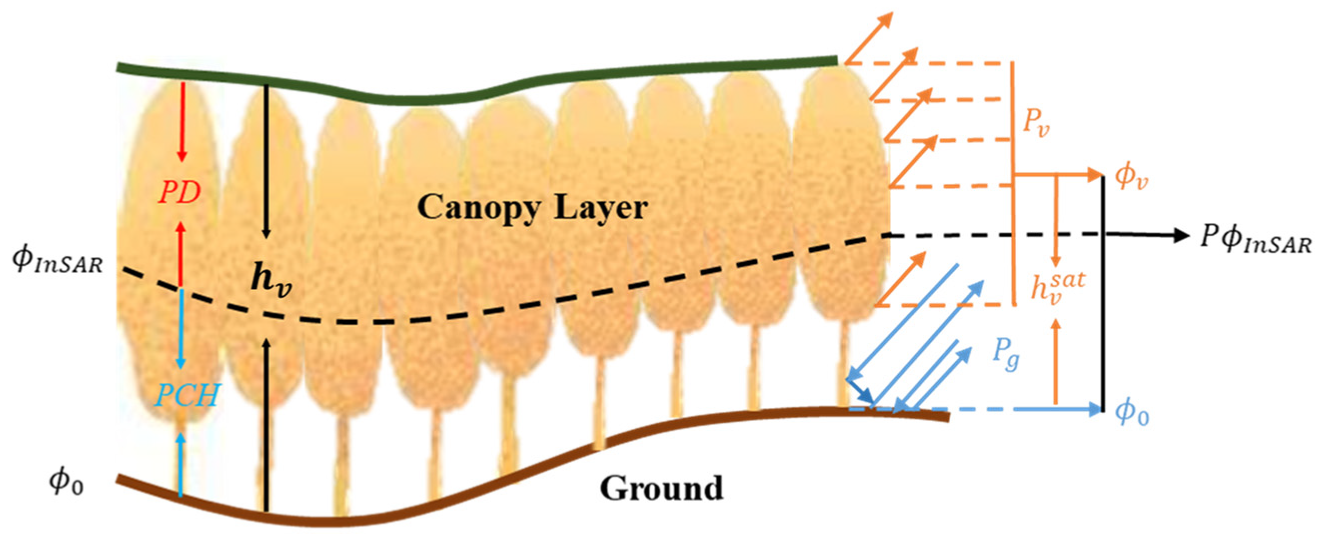
2.1. Inversion Model

The forward scattering model establishes the relationship between the forest biophysical parameters and the InSAR observables. Among the different scattering models, the RVoG model is the most widely used two-layer coherent scattering model, which expresses the InSAR coherence as [12,13]

$$\widehat{\gamma }=e^{i{\varphi }_0}\left(\widehat{{\gamma }_v}+\frac{\mu }{1+\mu }\left(1-\widehat{{\gamma }_v}\right)\right)$$

(1)

where ${\varphi }_0$ is the ground phase; $\mu$ denotes the GVR; and $\widehat{{\gamma }_v}$ represents the pure volume scattering coherence, which is given by

$$\widehat{{\gamma }_v}=\frac{{\int }_0^{h_v}\mathit{exp}\left(\frac{2\sigma z}{cos\theta }\right)\mathit{exp}\left(i{k}_{z}z\right)dz}{{\int }_0^{h_v}\mathit{exp}\left(\frac{2\sigma z}{cos\theta }\right)dz}$$

(2)

where $h_v$ is the canopy height; $\sigma$ is the mean extinction coefficient; $\theta$ represents the local incidence angle; and $k_z$ is the vertical wavenumber, which is expressed as

$$k_z=m\frac{2\pi B_{\perp }}{\lambda R\mathit{sin}\theta }$$

(3)

where $B_{\perp }$ is the length of the perpendicular baseline, $\lambda$ represents the wavelength, and $R$ is the slant range. For bistatic acquisitions, $m=1$, whereas for monostatic acquisitions, $m=2$. In the absence of ground contribution, Equation (1) can be written as

$$\widehat{\gamma }=e^{i{\varphi }_0}\widehat{{\gamma }_v}$$

(4)

where the unknown parameters are extinction and forest height, and the InSAR observation information is sufficient to solve the RVOG model by using (4). However, if the ground contribution exists, (1) cannot be solved directly from InSAR data. Therefore, in the next section, we introduce the GVR model derived from the InSAR backscattering to solve the RVoG inversion problem in the presence of ground contribution.

2.2. GVR Model Derived from InSAR Backscattering

According to the RVoG model, the scattering contribution from a forest scene can be attributed to the combination of the canopy layer and the sub-canopy ground (see Figure 1), which can be represented as

$$P{e}^{i{\varphi }_{InSAR}}=P_v{e}^{i{\varphi }_v}+P_g{e}^{i{\varphi }_0}$$

(5)

where $P_v$ represents volume scattering power, (saffron in Figure 1). $P_v$ derives from the backscattering contribution of canopy leaves and branches, whose average phase center is ${\varphi }_v$. $P_g$ represents the ground scattering power (blue in Figure 1). $P_g$ comes from the double-bounce scattering contribution between tree stems and ground surface as well as the surface scattering contribution on the ground, and their phase centers are all located at ${\varphi }_0$. Volume scattering and ground scattering contributions constitute together the InSAR backscattering signal (black in Figure 1), including the total backscattering power $P$ and the mean phase center of all scatterers in height direction, which is represented as the InSAR phase center ${\varphi }_{InSAR}$. If ground contribution exists, ${\varphi }_v$ is higher than ${\varphi }_{InSAR}$, as shown in Figure 1; otherwise, ${\varphi }_v$ equal ${\varphi }_{InSAR}$. From (5), ${\varphi }_{InSAR}$ can be expressed as

$${\varphi }_{InSAR}={\mathit{tan}}^{-1}\frac{\mathit{sin}{\varphi }_v+\mu \mathit{sin}{\varphi }_0}{\mathit{cos}{\varphi }_v+\mu \mathit{cos}{\varphi }_0}$$

(6)

In addition, ${\varphi }_{InSAR}$ can also be expressed as a function of the height:

$${\varphi }_{InSAR}=k_z\cdot PCH+{\varphi }_0$$

(7)

where $PCH$ is the InSAR phase center height in the forest, and the phase center of the volume scattering ${\varphi }_v$ can be represented as

$${\varphi }_v=k_z\cdot h_v^{sat}+{\varphi }_0$$

(8)

where $h_v^{sat}$ is the phase center height of the volume scattering, which can be derived from the RVoG backscattering model [23]:

$$P=\frac{P_v}{2\sigma /\mathit{cos}\theta }(1-e^{-\frac{2\sigma h_v}{\mathit{cos}\theta }})+P_g{h}_v{e}^{-\frac{2\sigma h_v}{\mathit{cos}\theta }}$$

(9)

From which, the volume phase center height can be defined where the backscattering power is maximal [23]:

$$h_v^{sat}=\frac{\mathit{cos}\theta (1+\mu )}{2\sigma \mu }.$$

(10)

To obtain $h_v^{sat}$, we introduce the penetration depth (PD), which is defined as the height deviation between the InSAR phase center and the top of the forest canopy [24]. As shown in Figure 1, in general, forest canopy height is equal to the sum of PD and PCH. Based on the empirical formula of extinction coefficient, the two-way penetration depth PD can be approximated as [12,13,24,25]

$$PD\approx \frac{\mathit{cos}\theta }{2\sigma }$$

(11)

By combining (6) and (8)–(11), the phase center of the forest ${\varphi }_{InSAR}$ can be expressed as

$${\varphi }_{InSAR}={\mathit{tan}}^{-1}\frac{\mathit{sin}(k_z\frac{PD(1+\mu )}{\mu }+{\varphi }_0)+\mu \mathit{sin}{\varphi }_0}{\mathit{cos}(k_z\frac{PD(1+\mu )}{\mu }+{\varphi }_0)+\mu \mathit{cos}{\varphi }_0}.$$

(12)

If an external DTM is available, ${\varphi }_0=k_z\cdot DTM$ can be obtained directly, and ${\varphi }_{InSAR}$ can be obtained from the unwrapped interferometric phase. Furthermore, if prior knowledge of the penetration depth is available, the GVR can be estimated.

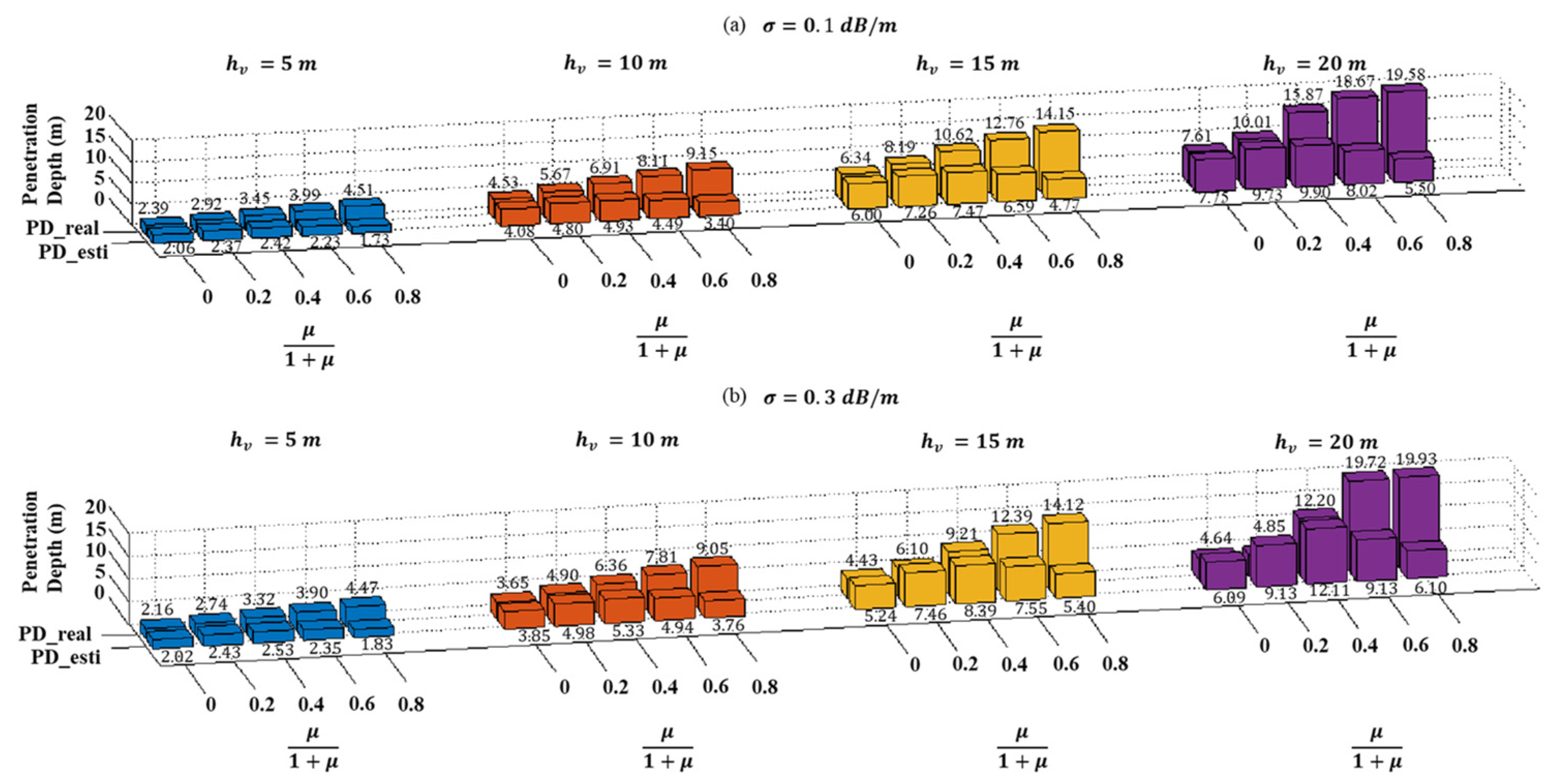
2.3. Approximate Estimation of Penetration Depth

According to the definition of PD (see Figure 1), it should be expressed as

$$PD=h_v-PCH.$$

(13)

where $h_v$ is the canopy height, which can be derived from a simplified model by assuming that there is no contribution from the ground and a null extinction [14,26]:

$$h_v=\frac{1}{k_z}(\arg \left(\widehat{\gamma }{e}^{-i{\varphi }_0}\right)+\eta (\pi -2{sin}^{-1}({\left|\widehat{\gamma }\right|}^{0.8}))).$$

(14)

This formula consists of two parts: the first part represents the phase center height and the second part is an approximation of the SINC function, which is a special form of zero extinction in (2). $\eta$ is a weighting factor that can compensate variations in structure, which is taken as 0.8 in this paper. Combining (13) and (14), the penetration depth can be approximate as

$$PD\approx 0.8(\pi -2{\mathit{sin}}^{-1}(|\widehat{\gamma }{|}^{0.8}\left)\right)/k_z$$

(15)

It should be noted that the estimated PD will be quite different from the real PD due to no ground contribution and null extinction assumptions. For further analysis, the InSAR complex coherence of forest is simulated by (1), and then the real penetration depth can be calculated from (13) according to the phase center height.

The estimated penetration depth can be obtained by (15) according to the simulated InSAR coherence amplitude. Other parameters include the vertical wavenumber of 0.2 rad/m and the incident angle of 30°. The comparison between the real PD and the estimated PD is shown in Figure 2a,b. Different colors correspond to different forest canopy heights, ranging from 5 m to 20 m with intervals of 5 m. Figure 2a,b have fixed extinction of 0.1 dB/m and 0.3 dB/m, respectively. For a given extinction and canopy height, the GVR gradually increases from left to right. Since complex coherence is used instead of pure volume coherence in (14), the complex coherence will gradually be higher than pure volume coherence as the GVR increases, resulting in a serious underestimation of the estimated PD. Compare with Figure 2a,b, the null extinction assumption leads to an overestimation of the estimated PD, which increases with the increase in extinction. Overall, the estimated PD is more accurate when GVR is small; however, there is serious underestimation when there is a strong ground contribution. The direct use of (14) to obtain canopy height will cause a large inversion deviation. Fortunately, when it is used to estimate GVR by (12), the retrieval of canopy height will not cause a large inversion error. The introduction of Formula (11) not only provides a rough estimation of the extinction coefficient but also restricts the range of extinction coefficient. First, it satisfies the basic law that the greater the PD, the stronger the ground contribution and the smaller the extinction. Secondly, it guarantees that when the PD is higher than 2 m, the extinction coefficient is within 0 to 0.22 dB/m with a 30° incident angle. This range is exactly the corresponding extinction range under the strong ground contribution and, combined with the estimated PD in Figure 2, even if the PD is seriously underestimated under strong ground contribution, the obtained extinction will not be too high, thus ensuring the reliability of the inversion process. The influence of PD error on forest height inversion is discussed in Section 5.3.

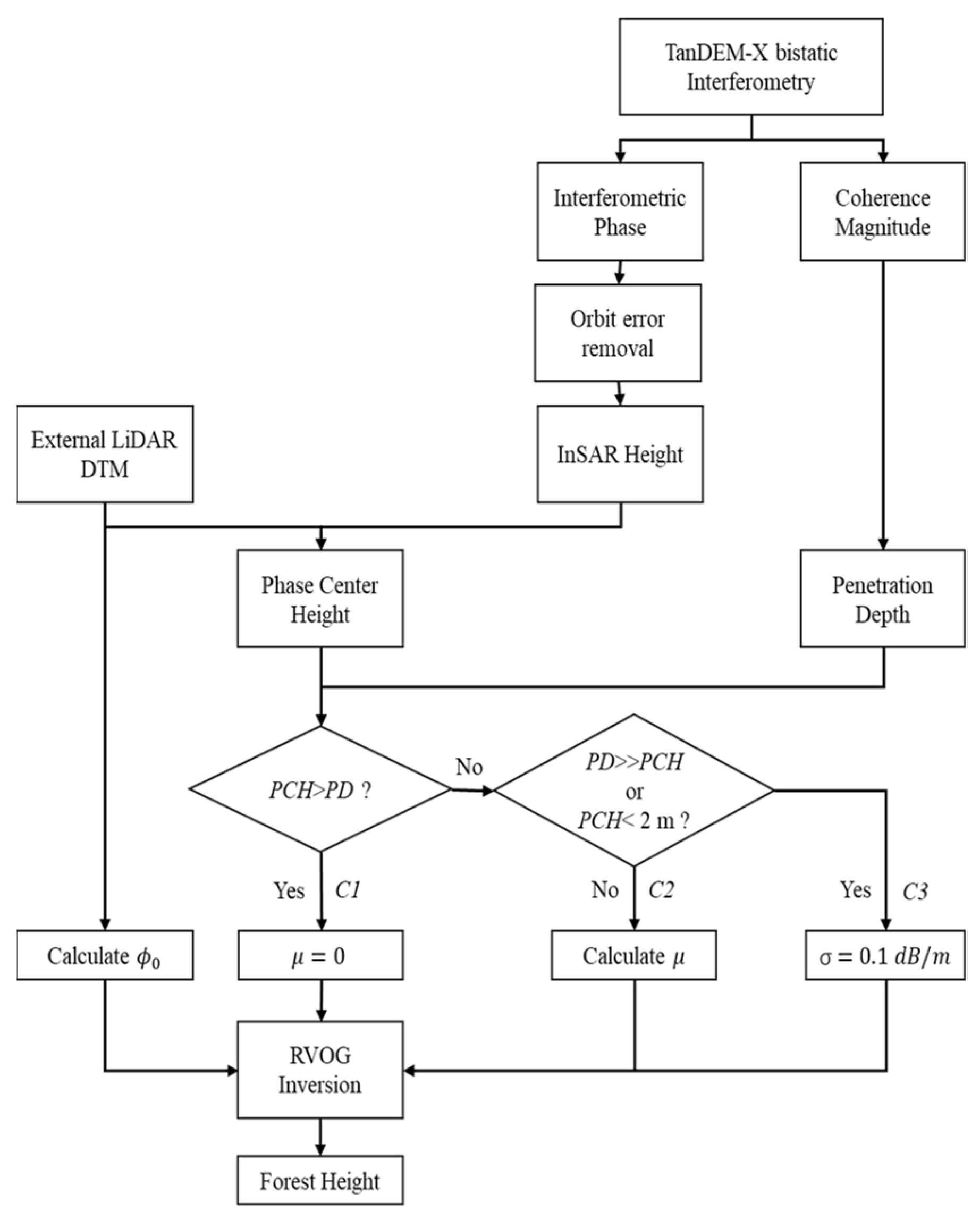
2.4. Forest Height Inversion

Due to the limited penetration capacity of X-band SAR signals, in many cases, the SAR signal cannot fully penetrate through the canopy and reach the ground. Hence, it is necessary to identify the different penetration conditions and design different inversion methods adapted to them. According to Praks’s work [27], microwave scattering in a forest can be considered as three cases:

(C1) Penetration depth shorter than half of the forest height: As shown in Figure 3, this situation usually occurs in dense and high forests with a large extinction coefficient, and without ground contribution. As mentioned before, forest canopy height equals the sum of PD and PCH, so if PD < PCH then PD < 0.5(PCH + PD), this case can be identified if PD is smaller than the PCH. The GVR then can be ignored, and the forest height can be estimated by (4) directly. Combined with Figure 2, it can be found that this rule corresponds to the forest with $\frac{\mu }{1+\mu }<0.2$, which has negligible ground contribution.

(C2) Penetration through the whole canopy: This situation usually occurs in sparse and low height forests with a small or moderate extinction coefficient, and both the GVR and extinction coefficient need to be considered (see Figure 3(C2)). This case can be identified if the phase center height is less than or equal to the penetration depth. The GVR can be estimated by (12) and then substituted into (1) to estimate the forest height. It is worth noting that the estimated PD will be seriously underestimated in the case of a large GVR; however, the corresponding PCH will still be lower than the estimated PD, and this rule can still be applied.

(C3) Strong ground contribution: This is not commonly seen in X-band SAR data; however, due to the very high spatial resolution of TanDEM-X satellites, strong ground contribution is also observed in sparse vegetation in dry environments, especially when the ground owns a large positive slope. In this case, PD will be much greater than PCH. However, due to the strong ground contribution, the estimated PD will be seriously underestimated. It is necessary to combine the situation of PCH for identification and it should be very close to the ground surface (see Figure 2: there is a huge deviation between the estimated PD and the real PD if PCH < 2 m). In this case, the GVR can no longer be obtained by (12) due to the serious underestimation of PD. However, this situation only occurs when the canopy layer has a very small or zero extinction; therefore, fixing a small value of extinction can solve the problem.

In conclusion, the overall methodology employed for forest height inversion is illustrated in Figure 4. The forest is firstly classified according to the estimated PD and PCH. If the penetration depth is less than or equal to the phase center height, the ground scattering contribution can be ignored. Otherwise, the GVR can be estimated from (13). GVR estimation from (12) is a nonlinear solution procedure. Due to the phase center height of volume scattering, $h_v^{sat}$ should be higher than the InSAR phase center height (PCH) and lower than the tree height; the range of GVR could then be determined by

$$PCH<PD\frac{(1+\mu )}{\mu }<PCH+PD.$$

(16)

The GVR of each pixel then can be estimated by finding a GVR such that the ${\varphi }_{InSAR}$ obtained from (12) is closest to the TanDEM-X observed value ${\varphi }_{InSAR}^0$:

$$\mathit{min}|\left|{\varphi }_{InSAR}-{\varphi }_{InSAR}^0\right|.$$

(17)

As shown in Table 1, in order to investigate the performance of the proposed method, three other existing RVoG-based methods [6,21,22] were also used to extract the forest height, making a total of four different cases:

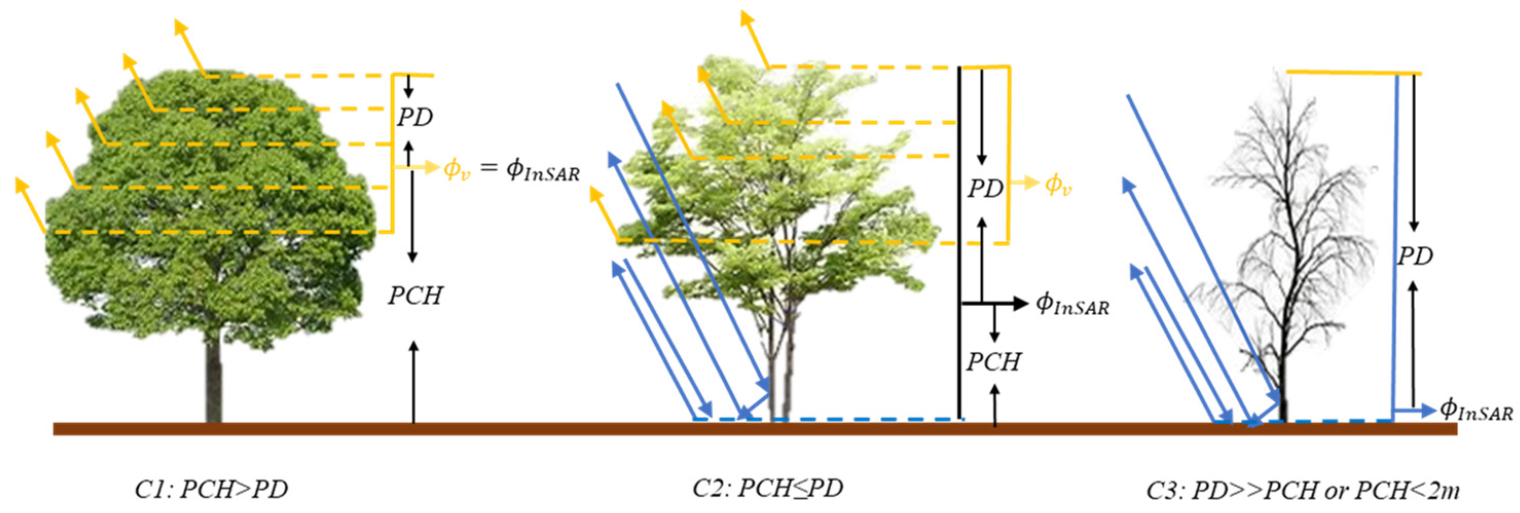
• Case one: Ground ignored, i.e., GVR = 0.
• Case two: Extinction fixed.
• Case three: GEDI simulation, i.e., introduce the LiDAR canopy height model (CHM) data.
• Case four: The method proposed in this work. If the penetration depth is shorter than forest height, the GVR is ignored. Otherwise, GVR is estimated from InSAR data with the GVR model.

Table 1. Different methods for retrieving RVoG model parameters.

Case	Method	Additional Data	RVoG Parameters
One	Ground ignored	None	$\mu =0$
Two	Extinction fixed	None	σ = 0.3 dB/m
Three	GEDI simulation	LiDAR CHM downsampled at intervals of 60 m in azimuth and 500 m in range	σ and $\mu$ maps interpolated from σ and $\mu$ values along simulated GEDI tracks
Four	Proposed method	None	If PD < PCH then $\mu$ = 0, if PD >> PCH or PCH < 2 m then σ = 0.1 dB/m; otherwise, $\mu$ from GVR model

Table 1. Different methods for retrieving RVoG model parameters.

Case	Method	Additional Data	RVoG Parameters
One	Ground ignored	None	$\mu =0$
Two	Extinction fixed	None	σ = 0.3 dB/m
Three	GEDI simulation	LiDAR CHM downsampled at intervals of 60 m in azimuth and 500 m in range	σ and $\mu$ maps interpolated from σ and $\mu$ values along simulated GEDI tracks
Four	Proposed method	None	If PD < PCH then $\mu$ = 0, if PD >> PCH or PCH < 2 m then σ = 0.1 dB/m; otherwise, $\mu$ from GVR model

In particular, for case two (fixed extinction), according to the existing works, the extinction coefficient was fixed to 0.3 dB/m. For case three (GEDI simulation), the method used in [22] was adopted, whose core idea is that the simulated spaceborne Global Ecosystem Dynamics Investigation (GEDI) LiDAR data are downsampled by airborne LiDAR data at intervals of 60 m in azimuth and 500 m in range, and then the simulated GEDI CHM product is used to invert the model parameters.

3. Test Sites and Experimental Data

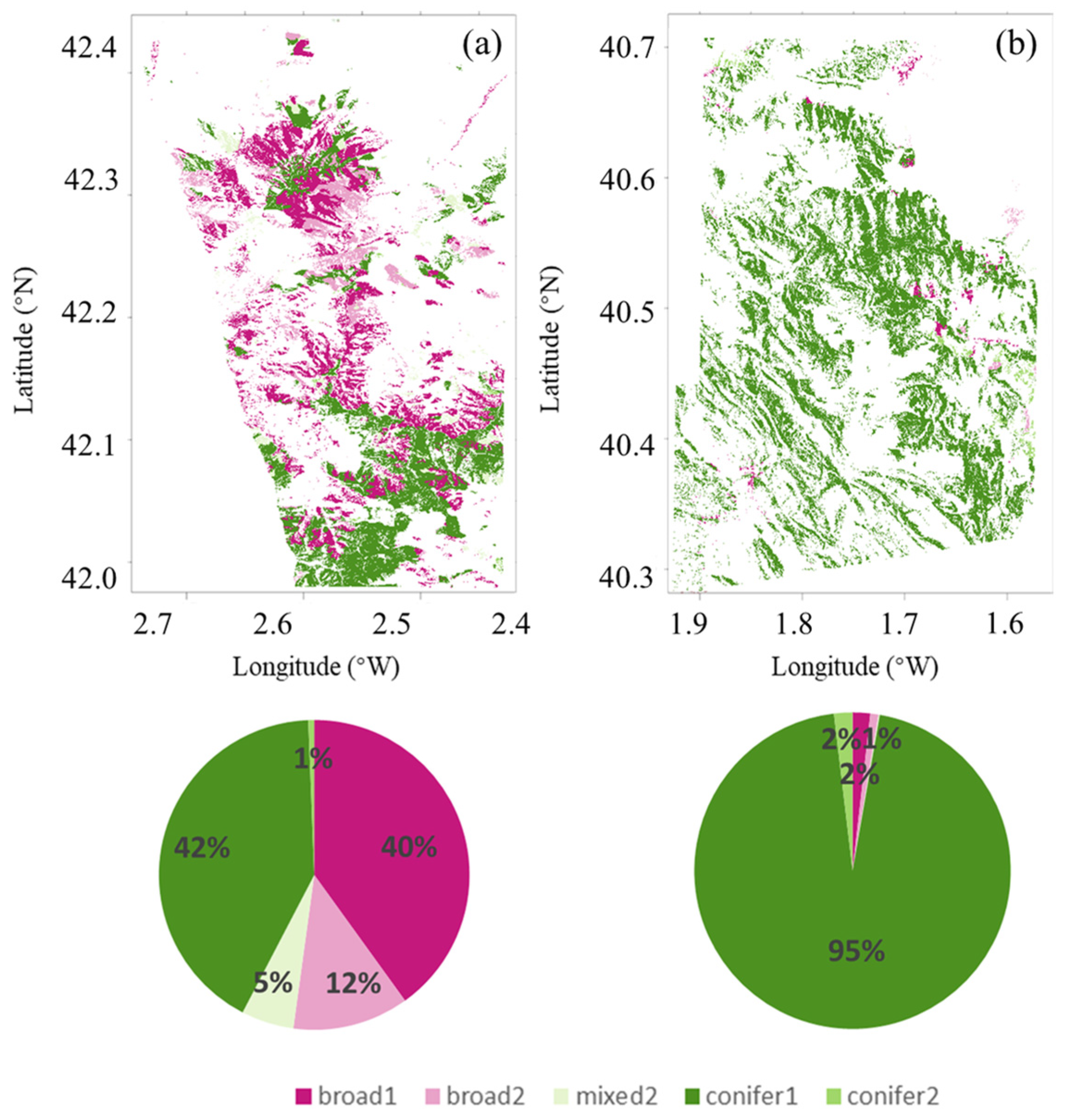
3.1. Test Sites

Two distinct sites, each representative of Mediterranean forests found in Spain [28,29] were selected for the evaluation of our proposed method (see Figure 5). The La Rioja site is situated within Sierra Cebollera, nestled in the Sistema Iberico mountain range. Covering an extension of 1350 km², the La Rioja site boasts a rich diversity of forest types, which include dense forests of broadleaved deciduous species like Quercus robur, Fagus sylvatica, and Fraxinus sp., and dense coniferous forests of Pinus sylvestris, as well as scattered sparse forests of Quercus ilex and Quercus faginea. This site encompasses 3215 stands of 18.0 ha on average (see Figure 5a). The second site, Teruel, is located in Sierra de Cuenca y Albarracín, which is also situated within the Sistema Ibérico mountain range. Encompassing an area of 1100 km², the Teruel site is characterized by dense coniferous forests of Pinus sylvestris, P. nigra, and P. pinaster with just some sporadic patches of sparse juniper forests and broadleaved Quercus sp. (see Figure 5b). The Teruel site comprises a total of 3080 stands, with an average size of 34.4 ha. LiDAR measurements from Gómez’s study [28] reveal that the majority of trees at both sites do not exceed 20 m in height.

3.2. LiDAR Data

The airborne LiDAR data were acquired between 2009 and 2015 by the Spanish National Plan for Territory Observation (PNOT) [30] with 0.5 points/m². The LiDAR-derived forest height data with a resolution of 10 m were generated to validate the retrieved forest height, and the LiDAR DTM data with a resolution of 5 m were used to simulate the ground interferometric phase.

3.3. TanDEM-X InSAR Data

The TanDEM-X SAR data acquired in the HH polarization in coregistered single-look slant-range complex (CoSSC) format enabled the direct generation of the interferograms, with its coverage marked with blue rectangles in Figure 5. Two TanDEM-X InSAR pairs acquired in the leaf-off period and with a suitable height of ambiguity (HoA) were chosen (see

Table 2. TanDEM-X datasets for the two test sites.

Area	Date	HoA (m)	Look Angle (°)
La Rioja	28 December 2012	36.58	34.73
Teruel	23 October 2012	32.29	37.10

). The coherence was estimated using a 9 × 9 boxcar window, and common band filtering [31] was carried out to compensate the geometric decorrelation. Signal-to-noise ratio (SNR) correction [6] and quantization error compensation [32] were then applied to further compensate the corresponding decorrelations. The LiDAR DTM was used to simulate the bare ground interferometric phase and remove the orbit error phase by the fitting of a polynomial [33]. The final product uses $4\times 4$ multi-looks with a spatial resolution of 10 m $\times$ 10 m.

4. Results

4.1. Penetration Performance in Two Sites

Both the extinction coefficient and the GVR are related to the penetration performance of microwaves in forest. The smaller the extinction, the stronger the penetration and the ground scattering contribution. Therefore, it is necessary to introduce the penetration conditions in the test sites before analyzing the influence of different model parameter acquisition methods on the RVoG inversion. To this end, we define the penetration ratio as the ratio of the penetration depth (LiDAR tree height minus InSAR height) to the LiDAR tree height. The histograms of the penetration ratio vs. the LiDAR tree height are shown in Figure 6 for the two test sites.

To demonstrate the penetration of the X-band for the different types of forest, we rasterized the forest type data, then geocoded it into SAR coordinates, and resampled it to each pixel (see Figure 7). According to the forest type of each pixel, we divided the La Rioja test site into two classes, with one consisting of conifer stands of different densities (conifer 1 and conifer 2) and the other one consisting of broadleaved stands of different densities (broad 1 and broad 2). The histograms corresponding to these classes are shown in Figure 6c and Figure 6d, respectively. From Figure 6a, it is observed that most of the tree heights at the La Rioja test site are less than 18 m and are concentrated in the 3–9 m range. In examining Figure 6c,d, it is found that the trees between 3 m and 9 m are mainly broadleaved, which are almost completely penetrated by the X-band radar. The tree heights for the coniferous forest are mainly distributed in the 9–18 m range, where the penetration depth decreases linearly as the tree height increases. This phenomenon also occurs in some of the broadleaved forest with tree height greater than 9 m. Almost all the areas of broadleaf forest exhibit penetration ratios higher than 0.5, and only a few areas of coniferous forest show penetration ratios lower than 0.5. This means that the phase center height is less than half of the tree height in most areas of the La Rioja test site, where both the GVR and extinction coefficient play a critical role in the RVoG inversion.

From Figure 6b, it is observed that the tree height is concentrated in the range of 6–18 m at the Teruel test site. Although the penetration ratio is still higher than 0.5 in most areas, penetration is much lower than at the La Rioja test site compared to Figure 6a, in which most pixels have penetration ratios higher than 0.8.

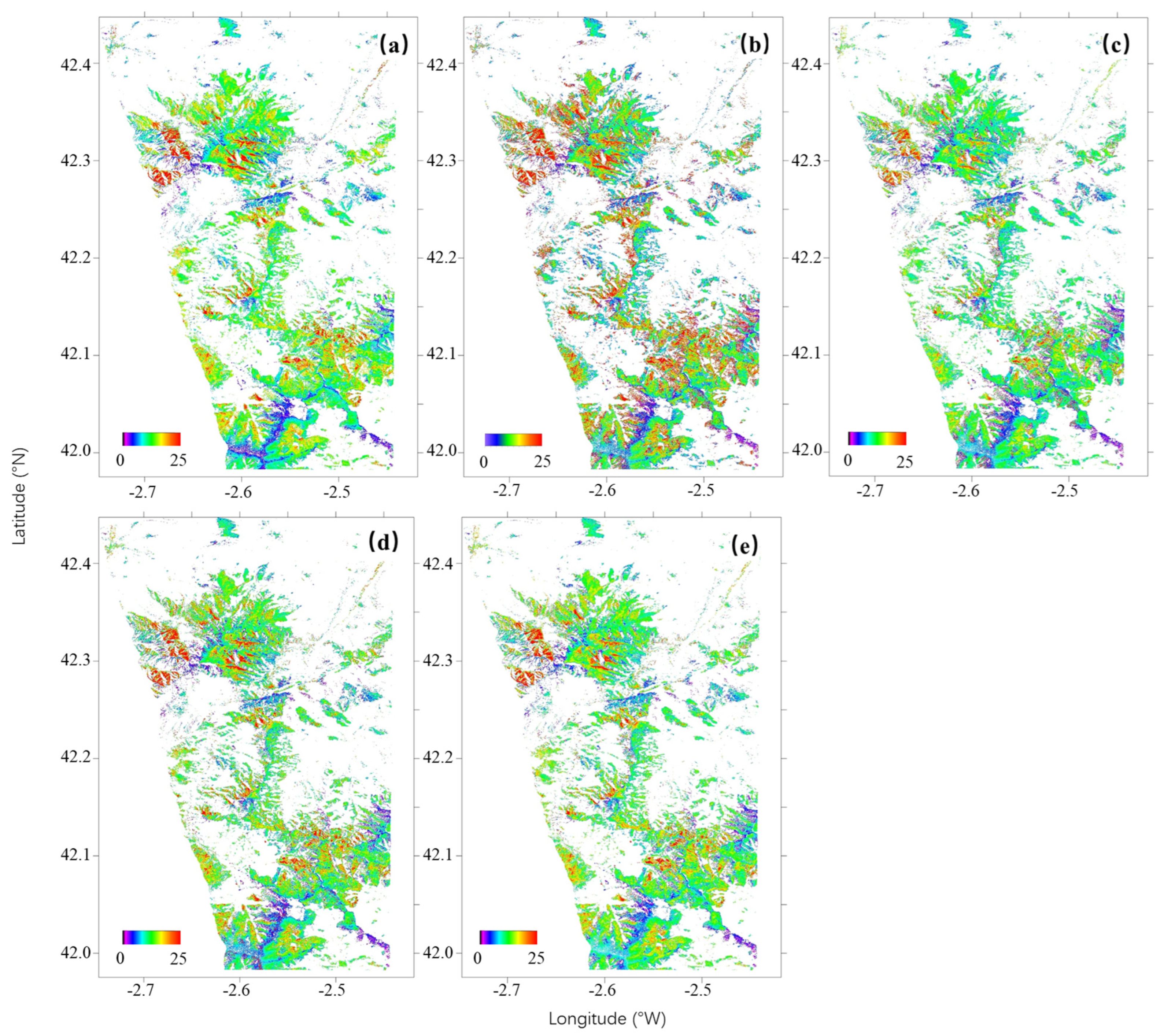
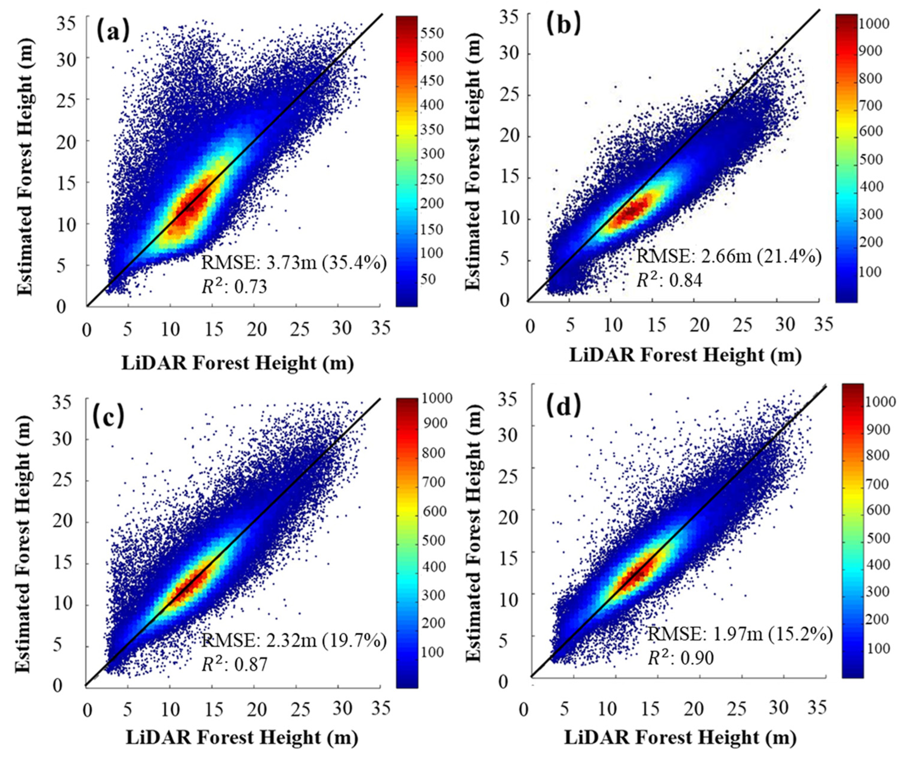
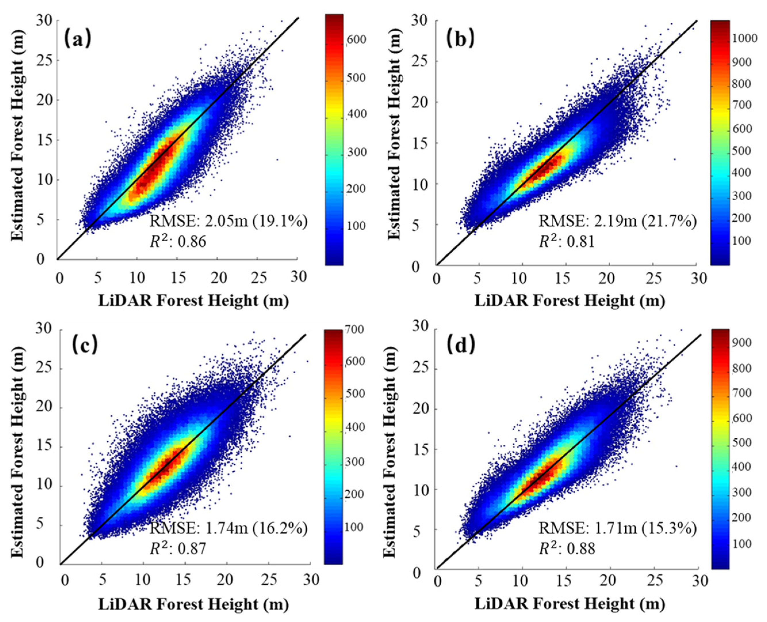
4.2. Inversion at the La Rioja Test Site

The inversion results for the four methods defined in Section 2.3 (Table 1) are shown in Figure 8, where the LiDAR-derived forest height is also shown for comparison. The retrieved height shows a high spatial similarity with the LiDAR height, except for the results from case one (ground ignored), in which significant overestimation occurs in some areas due to the inappropriate GVR assumption. The scatter plots computed for validation in the four cases are shown in Figure 9, where the $R^2$ coefficient of determination and the root-mean-square error (RMSE) obtained from the comparison of the LiDAR heights and TanDEM-X-retrieved heights are also listed. A 5 × 5 (50 m × 50 m) sliding window is used for an accuracy evaluation. The inversion accuracies for the four cases are quite different in the La Rioja test site, with the RMSE ranging from 1.97 m to 3.73 m and the $R^2$ ranging from 0.73 to 0.90. The worst inversion results appear in case one (ground ignored method). From Figure 9a, it is observed that the diagonal line is located above the dense scatter plot area (dark red area) when the tree heights are below 12 m. There is strong penetration in the La Rioja test site with tree heights below 12 m, and this underestimation is caused by ignoring the ground contribution. There is no significant deviation in areas with tree heights above 12 m, indicating that ignoring the ground contribution is feasible in tall forests, where the X-band radar only penetrates into the canopy. There are some overestimated discrete plots in the areas with tree heights below 15 m. When combined with the spatial distribution map of the inversion results, it can be found that all these areas have a large positive range slope. The slope effects are discussed in Section 5.2. Figure 9b shows the inversion results for case two (extinction fixed method), where the excessive extinction coefficient causes overall underestimation of the inversion results, and with the increase in the tree height, the underestimation becomes more relevant. The proposed method achieves the best inversion performance. Compared with the result for case three (GEDI simulation method), both the spatial distribution map and the scatter plot are highly consistent. This means that both of them can accurately estimate the model parameters, but the proposed method does not depend on additional data.

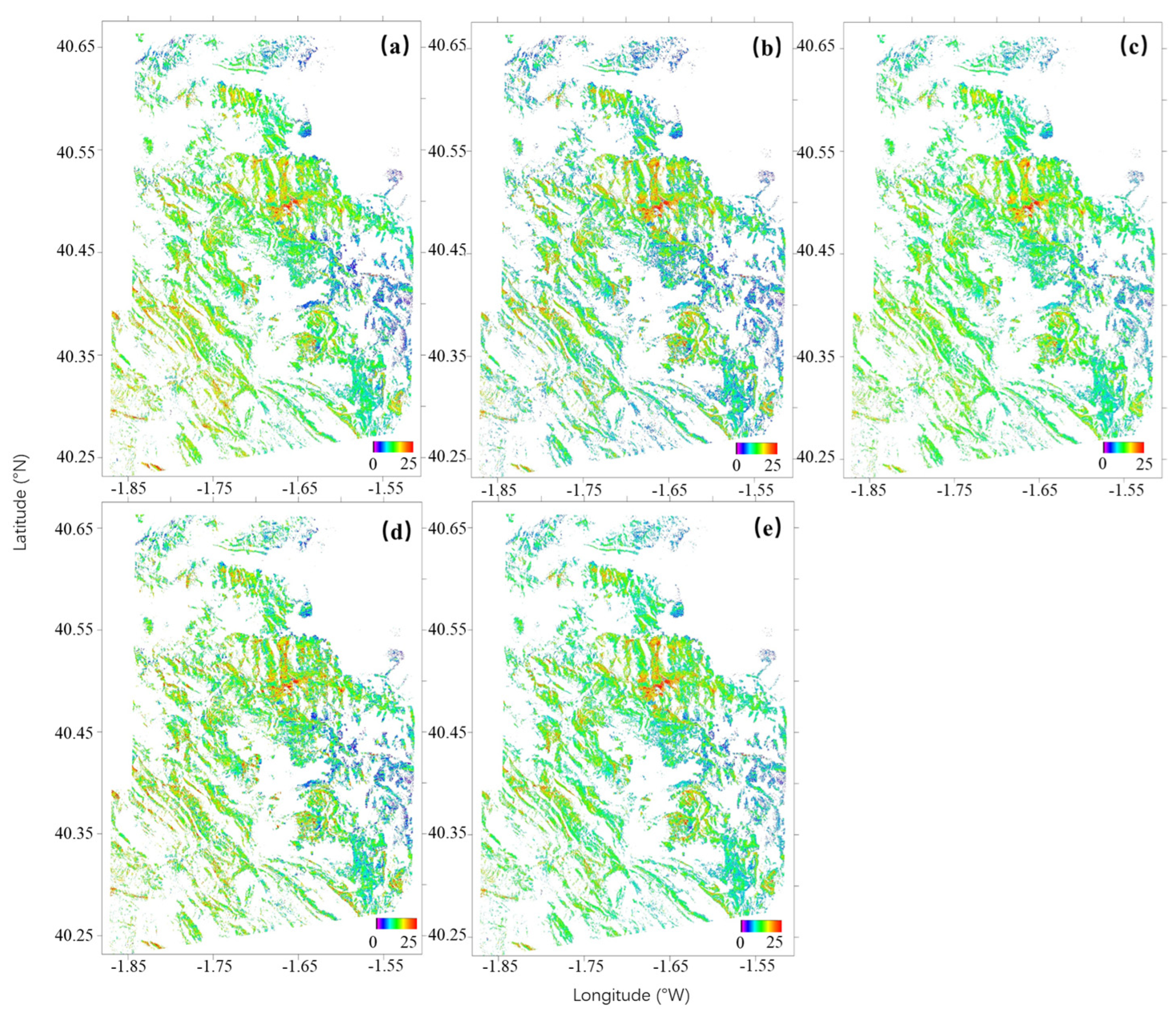
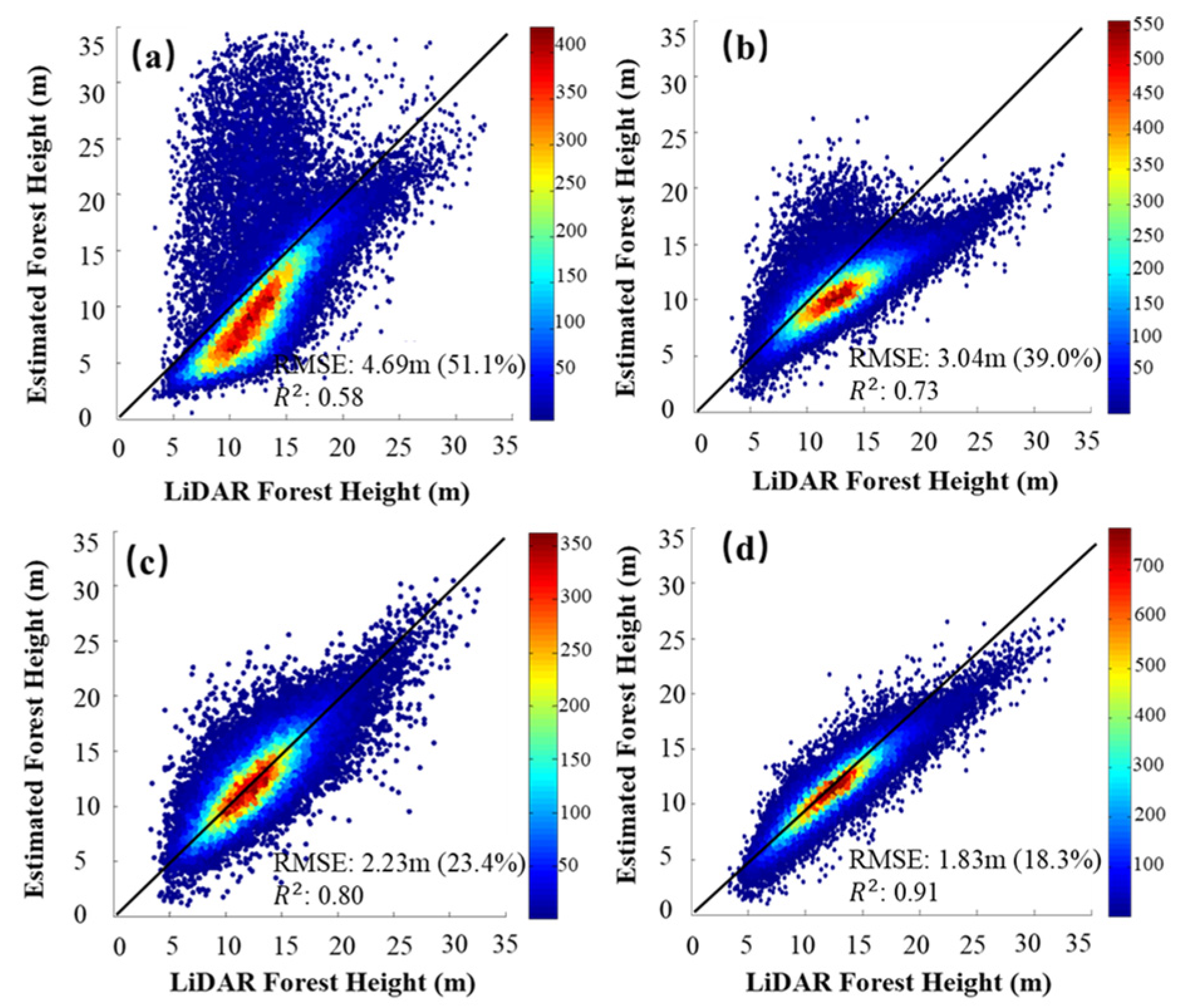
4.3. Inversion at the Teruel Test Site

The retrieved forest heights for the four cases show high spatial consistency with the LiDAR heights (see Figure 10), and the inversion accuracies for the four cases are also comparable (see Figure 11), with the RMSE ranging from 1.71 m to 2.19 m and the $R^2$ ranging from 0.81 to 0.88. The similar results indicate that the spatial variations in the GVR and extinction coefficient are limited and very close to our assumptions. On the one hand, it can be seen from Figure 7 that the Teruel site is much more homogeneous (in terms of forest species) than the La Rioja site. It indicates that the model parameters have less spatial variation in a homogeneous forest stand than in a complex forest. On the other hand, in comparing the inversion results of case one (ground ignored method) in the two sites, the ground contribution in Teruel is not as significant as in La Rioja, and a significant underestimation appears in the inversion tree height for the 9 m to 12 m range in Teruel, where the penetration ratio is greater than 0.5 (Figure 6b). Similarly, by comparing the inversion results of case two (extinction fixed method) in the two sites, we find that the extinction coefficient in Teruel is closer to our assumption (0.3 dB) than in La Rioja, which is consistent with the difference in the penetration performance between the two sites.

5. Discussion

5.1. Retrieved Height with Full Penetration

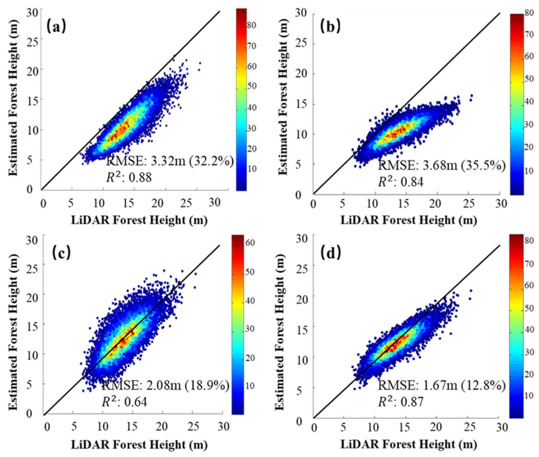
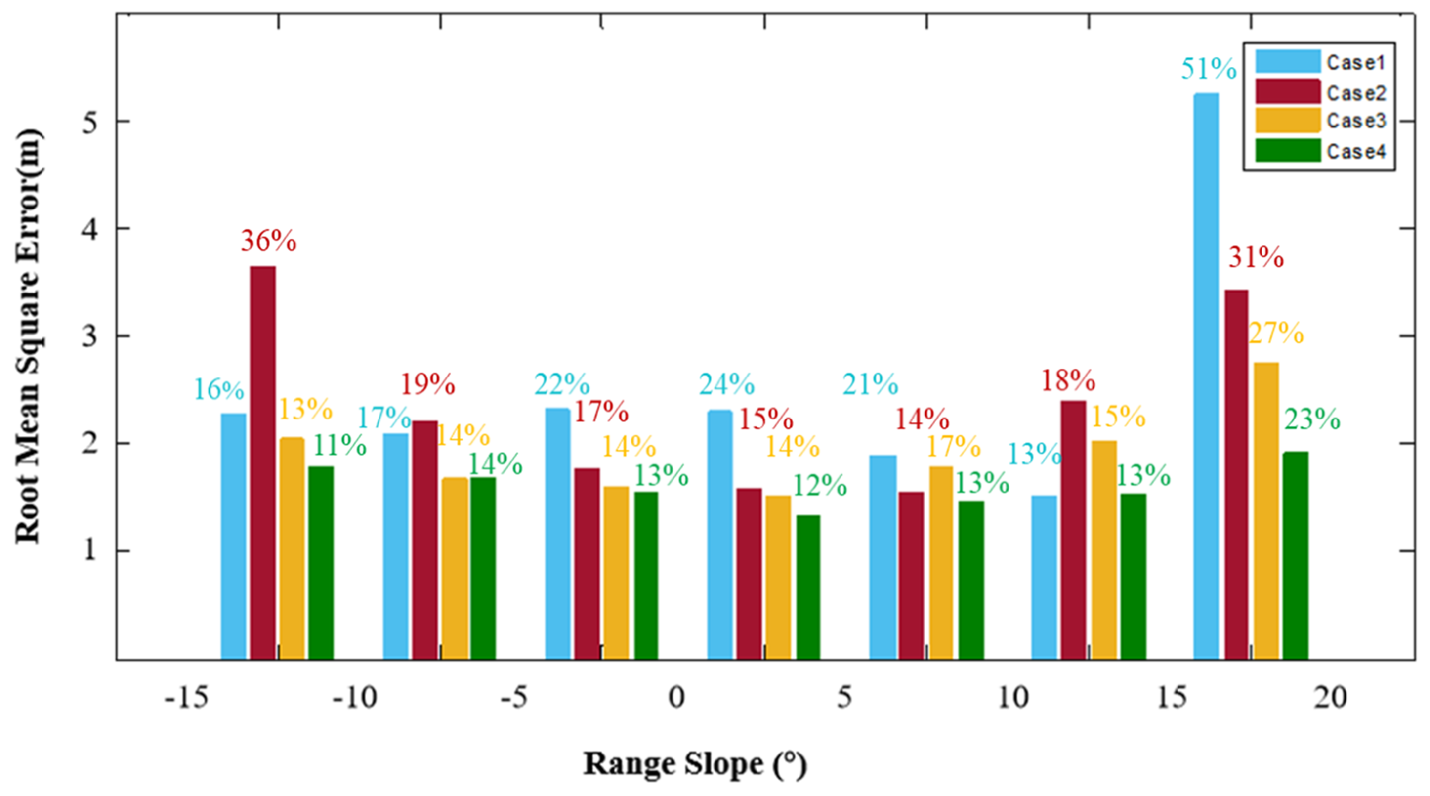
To further demonstrate the effectiveness of the proposed GVR estimation method, we consider in this section the case of strong penetration, where the GVR plays an important role in the RVoG inversion. After masking the area where the phase center was above half of the tree height, scatter plots of the retrieved height versus LiDAR heights in the two test sites were generated and are shown in Figure 12 and Figure 13, respectively. The RMSE ranges from 1.83 m to 4.69 m at the La Rioja test site and from 1.67 m to 3.68 m at the Teruel test site. The inversion accuracy for case one (ground ignored) and case two (extinction fixed) is significantly reduced. This indicates that there was a large GVR when penetrating through the canopy. However, there is a high level of inversion accuracy for both case three (GEDI simulation) and the proposed method in such a situation, which demonstrates the effectiveness of the proposed GVR estimation method. Compared with the result for case three (GDEI simulation) and the proposed method, it can be seen that the inversion result of the proposed method has fewer discrete plots and R² is improved from 0.80 to 0.91 in the La Rioja site and from 0.64 to 0.87 in the Teruel site. The proposed method can realize a pixel-by-pixel model parameters estimation; however, spaceborne LiDAR can only provide observations along transects or tracks. As a result, the accuracy of model parameter acquisition will gradually decrease with the distance between the pixels and LiDAR observations. Therefore, the inversion results of the proposed method will be more convergent and have fewer discrete points when compared with the GEDI method.

5.2. Slope Effect

Many overestimated plots with tree height below 15 m were observed in the scatter plot for case one (ground ignored) at the La Rioja test site. When compared with the height spatial distribution map, it is apparent that most of these overestimations appear in areas with positive range slope. To analyze the influence of range slope on the inversion of the model parameters, in Figure 14, the RMSE of the inversion results are addressed for the four cases but with range slope ranging between −15° and 20° at 5° intervals. From this, we focus on the areas with a slope below 5°, which can be considered as areas of flat or gentle topography where there is improvement in all methods tested at the La Rioja test site. The proposed method achieves the lowest RMSE (1.34 m), which suggests that it is the optimal method provided that range slope effects can be ignored. Is it important to note that the range of tree heights in all range slope intervals is similar (i.e., mainly from 3 m to 18 m).

The inversion accuracy for case one (ground ignored) decreases notably when the slope exceeds 15°, which is consistent with the findings mentioned above in that ignoring the ground scattering contribution leads to significant overestimation in areas with large positive range slopes. However, the other three cases are not significantly affected, indicating that the effect of positive range slope can be mitigated by giving an appropriate GVR. By comparing with the other cases, it is found that case two (fixed extinction) is affected the most by the slope, and case three, which adopts the fusion of simulated GEDI LiDAR data and TanDEM-X InSAR data to obtain the RVoG model parameters, is less affected by the slope, while the proposed method is affected the least by the slope. This means that the part of the RVoG inversion deviation caused by the slope can be mitigated by adjusting the GVR, and the proposed method can maintain a stable RVoG inversion in such a case.

5.3. Influence of PD Estimation Error on Canopy Height Inversion

The estimated penetration depth obtained based on the SINC model is expected to deviate from the real penetration depth. The effects of this deviation on the forest height inversion need to be analyzed to ensure that this would not introduce a larger model error than fixing inappropriate model parameters. To ensure that it can reflect the full situation in a real scenario, we used a smaller parameter interval than the simulation in Section 2.3. We also simulated the complex coherence of the 5 m to 25 m tree height at 0.5 m intervals from the RVoG model, with a moderate extinction (0.2 dB/m or 0.3 dB/m) and strong ground scattering ($\frac{\mu }{1+\mu }$ was varied from 0.3 to 0.8, with intervals of 0.02). Other simulation parameters include the vertical wavenumber of 0.2 rad/m and the incident angle of 30°. The estimated PD can then be derived from the amplitude of the simulated complex coherence by (15), and the real PD could be obtained by

$$P{D}_{real}=h_{vsim}-PC{H}_{sim}$$

(18)

where $h_{vsim}$ is the simulated tree height and $PC{H}_{sim}$ is the simulated InSAR height. Both ${PD}_{esti}$ and $PC{H}_{sim}$ were used to calculate the simulated GVR by (12). The simulated tree height inversion result could then be derived from (1) by using the simulated GVR. In order to better demonstrate the influence of the PD estimation error on the canopy height inversion, we introduced the relative precision (RP) to demonstrate the inversion accuracy. It can be expressed as

$$RP=\left(1-\frac{\left|Real-Esti\right|}{Real}\right)\ast 100\%$$

(19)

where Real represents the true value and Esti represents the estimated value. Figure 15a,c show the difference between the estimated penetration depth based on the SINC model and the real penetration depth. It is clear that the deviation increases as the ground scattering contribution increases due to the zero-ground contribution assumption in the SINC model. However, the canopy height inversion results are less affected by the deviation of estimated penetration depth. As Figure 15b,d show, the relative deviation of the tree height inversion does not exceed 25%. Large inversion deviation only occurs in the combination of extreme model parameters and tall vegetation, where the phase center height is close to half of the tree height. For most natural forest scenes and low vegetation, the relative deviation does not exceed 10%.

5.4. Robustness and Error Sources of the Proposed Inversion Framework

To prove the robustness of the proposed inversion framework, we employed three other distinct methods for retrieving the model parameters: (1) neglecting ground contributions, which demonstrates the impact of inaccurate GVR on canopy height inversion; (2) fixing a large extinction coefficient, which represents the effects of inaccurate extinction coefficient on canopy height inversion; and (3) spaceborne LiDAR CHM-derived model parameters, ensuring the accurate acquisition of both GVR and extinction coefficient values (see Table 1). Moreover, in Section 5.3 we employed a Monte Carlo method to simulate the differences between our proposed inversion method (with GVR estimation) and the RVOG model across various forest scenarios. This analysis provided theoretical evidence for the effectiveness of our approach. Collectively, the comparison experiments conducted above fully demonstrate the reliability and robustness of the proposed GVR model and InSAR inversion framework for canopy height estimation. Moreover, to demonstrate the reliability of our inversion results, we conducted a comparative analysis with Qi’s research [22] (see

Table 3. Comparison of inversion accuracy between our study and Qi’s study.

Studies/Cases	Forest Type	RMSE (m)	RMSE (%)	Correlation Coefficient
Qi’s/μ = 0	Coniferous forest	6.83	17.7	0.53
	Broadleaved forest	6.22	25.9	0.32
Ours/μ = 0	Coniferous forest	2.05	19.1	0.86
	Coniferous and broadleaved forest	3.73	35.4	0.73
Qi’s/μ = 0, σ from GEDI	Coniferous forest	6.03	15.6	0.60
	Broadleaved forest	4.21	17.5	0.50
Ours/σ fixed as 0.3 dB/m	Coniferous forest	2.19	21.7	0.81
	Coniferous and broadleaved forest	2.66	21.4	0.84
Qi’s/ μ, σ from simulated GEDI	Coniferous forest	4.30	13.1	0.44
	Broadleaved forest	2.66	11.1	0.68
Ours/μ, σ from simulated GEDI	Coniferous forest	1.74	16.2	0.87
	Coniferous and broadleaved forest	2.32	19.7	0.87
Ours/Proposed Inversion Framework	Coniferous forest	1.71	15.3	0.88
	Coniferous and broadleaved forest	1.97	15.2	0.90

). Both studies exhibited similar performance when applying the same methodology. Notably, the least accurate inversions were observed in broadleaved forests when neglecting ground contributions. Besides our proposed approach, the most accurate inversion results were obtained using simulated GEDI data. Furthermore, both studies showed similar accuracy in inverting the three methods within the coniferous forest, while a significant disparity was observed in the case of broadleaved forests. The inversion accuracy of the same method in two studies is close to but not completely the same, and it should be noted that direct comparisons should be made cautiously due to differences in study conditions, such as statistical spatial resolution, baseline, validation data, and forest types.

This paper primarily explores the impact of RVOG model parameters (extinction coefficient and GVR) on canopy height inversion. To eliminate the influence of other factors, we initially compensated the main error sources of TanDEM-X InSAR data: signal-to-noise ratio (SNR) decorrelation and quantization decorrelation, as documented in the existing literature [6,30]. For the selection of the spatial baseline, we drew upon the research of Kugler [19] and Chen [17] opting for a baseline with HOA approximately 30 m, ensuring that it fell within the most suitable range for canopy height inversion, between $h_v$ to 3 $h_v$. Additionally, as advised by Olesk’s research [34], we selected acquision data during the leaf-off season to avoid seasonal influences. To minimize the impact of range slope, we implemented the S-RVOG model [35] and corrected $k_z$ according to Kugler’s research [19], and we still observed residual effects associated with the range slop in our results. In Section 5.2, we conducted an in-depth analysis of the influence of range slope on canopy height inversion by categorizing the outcomes based on different range slope values. In the absence of range slope influence, the RMSE was reduced to 1.34 m (12%), closely approaching the theoretical accuracy of 10% of the RVOG model.

6. Conclusions

In this paper, a GVR estimation method based on InSAR data was proposed, which allows the RVoG inversion to be achieved from single-baseline InSAR data without any model assumption or other prior information except for an external DTM. The effectiveness of the proposed method was demonstrated in both real-data and simulation experiments.

The proposed method establishes a DTM-assisted RVoG inversion framework based on single-baseline InSAR data. For a long time series, the terrain can be considered stable while the forest is changing. As a result, the proposed method is suitable for forest height mapping with a high refresh rate, as well as for change monitoring, in regions with available high-precision DTMs. The proposed method can also be combined with low-frequency SAR data, using the DTM inverted by the low-frequency SAR data, and it can also be applied to some other methods that can obtain a DTM from InSAR data, such as multi-squint [36] and the penetration depth compensation-based method [37].

The proposed GVR estimation method is also applicable to forest height inversion with low-frequency PolInSAR data, which enables the inversion process to be conducted without assuming that a certain polarization channel does not contain a ground contribution, and the GVR can be generated using the data of any polarization channel to obtain the pure volume scattering coherence.

There are some limitations to the proposed method, such as the fact that the proposed GVR estimation method is highly nonlinear and requires some constraints to be added to avoid falling into local optima. Moreover, the proposed method is based on the RVoG model, without considering the influence of the vegetation vertical structure. The applicability for large-scale forest height inversion also needs to be further validated.

References

1. Schlund, M.; Erasmi, S.; Scipal, K. Comparison of Aboveground Biomass Estimation From InSAR and LiDAR Canopy Height Models in Tropical Forests. IEEE Geosci. Remote Sens. Lett. 2020, 17, 367–371. [Google Scholar] [CrossRef]
2. Nelson, R.; Margolis, H.; Montesano, P.; Sun, G.; Cook, B.; Corp, L.; Andersen, H.-E.; deJong, B.; Pellat, F.P.; Fickel, T.; et al. Lidar-Based Estimates of Aboveground Biomass in the Continental US and Mexico Using Ground, Airborne, and Satellite Observations. Remote Sens. Environ. 2017, 188, 127–140. [Google Scholar] [CrossRef]
3. Thomas, R.Q.; Hurtt, G.C.; Dubayah, R.; Schilz, M.H. Using Lidar Data and a Height-Structured Ecosystem Model to Estimate Forest Carbon Stocks and Fluxes over Mountainous Terrain. Can. J. Remote Sens. 2008, 34, S351–S363. [Google Scholar] [CrossRef]
4. Lagomasino, D.; Fatoyinbo, T.; Lee, S.; Feliciano, E.; Trettin, C.; Shapiro, A.; Mangora, M.M. Measuring Mangrove Carbon Loss and Gain in Deltas. Environ. Res. Lett. 2019, 14, 025002. [Google Scholar] [CrossRef]
5. Askne, J.; Fransson, J.; Santoro, M.; Soja, M.; Ulander, L. Model-Based Biomass Estimation of a Hemi-Boreal Forest from Multitemporal TanDEM-X Acquisitions. Remote Sens. 2013, 5, 5574–5597. [Google Scholar] [CrossRef]
6. Kugler, F.; Schulze, D.; Hajnsek, I.; Pretzsch, H.; Papathanassiou, K.P. TanDEM-X Pol-InSAR Performance for Forest Height Estimation. IEEE Trans. Geosci. Remote Sens. 2014, 52, 6404–6422. [Google Scholar] [CrossRef]
7. Treuhaft, R.; Gonçalves, F.; dos Santos, J.R.; Keller, M.; Palace, M.; Madsen, S.N.; Sullivan, F.; Graça, P.M.L.A. Tropical-Forest Biomass Estimation at X-Band From the Spaceborne TanDEM-X Interferometer. IEEE Geosci. Remote Sens. Lett. 2015, 12, 239–243. [Google Scholar] [CrossRef]
8. Lei, Y.; Treuhaft, R.; Gonçalves, F. Automated Estimation of Forest Height and Underlying Topography over a Brazilian Tropical Forest with Single-Baseline Single-Polarization TanDEM-X SAR Interferometry. Remote Sens. Environ. 2021, 252, 112132. [Google Scholar] [CrossRef]
9. Lei, Y.; Treuhaft, R.; Keller, M.; dos-Santos, M.; Goncalves, F. Quantification of Selective Logging in Tropical Forest with Spaceborne SAR Interferometry. Remote Sens. Environ. Interdiscip. J. 2018, 221, 167–183. [Google Scholar] [CrossRef]
10. Shiroma, G.H.X.; Lavalle, M. Digital Terrain, Surface, and Canopy Height Models From InSAR Backscatter-Height Histograms. IEEE Trans. Geosci. Remote Sens. 2020, 58, 3754–3777. [Google Scholar] [CrossRef]
11. Treuhaft, R.N.; Chapman, B.D.; Santos, J.D.; GonçAlves, F.G.; Dutra, L.V.; GraçA, P.; Drake, J.B. Vegetation Profiles in Tropical Forests from Multibaseline Interferometric Synthetic Aperture Radar, Field, and Lidar Measurements. J. Geophys. Res. 2009, 114, D23110. [Google Scholar] [CrossRef]
12. Treuhaft, R.N.; Madsen, S.N.; Moghaddam, M.; Zyl, J.J. van Vegetation Characteristics and Underlying Topography from Interferometric Radar. Radio Sci. 1996, 31, 1449–1485. [Google Scholar] [CrossRef]
13. Papathanassiou, K.P.; Cloude, S.R. Single-Baseline Polarimetric SAR Interferometry. IEEE Trans. Geosci. Remote Sens. 2001, 39, 2352–2363. [Google Scholar] [CrossRef]
14. Chen, H.; Cloude, S.R.; Goodenough, D.G. Forest Canopy Height Estimation Using Tandem-X Coherence Data. IEEE J. Sel. Top. Appl. Earth Obs. Remote Sens. 2016, 9, 3177–3188. [Google Scholar] [CrossRef]
15. Olesk, A.; Praks, J.; Antropov, O.; Zalite, K.; Arumäe, T.; Voormansik, K. Interferometric SAR Coherence Models for Characterization of Hemiboreal Forests Using TanDEM-X Data. Remote Sens. 2016, 8, 700. [Google Scholar] [CrossRef]
16. Schlund, M.; Magdon, P.; Eaton, B.; Aumann, C.; Erasmi, S. Canopy Height Estimation with TanDEM-X in Temperate and Boreal Forests. Int. J. Appl. Earth Obs. Geoinf. 2019, 82, 101904. [Google Scholar] [CrossRef]
17. Chen, H.; Cloude, S.R.; Goodenough, D.G.; Hill, D.A.; Nesdoly, A. Radar Forest Height Estimation in Mountainous Terrain Using Tandem-X Coherence Data. IEEE J. Sel. Top. Appl. Earth Obs. Remote Sens. 2018, 11, 3443–3452. [Google Scholar] [CrossRef]
18. Praks, J.; Kugler, F.; Papathanassiou, K.P.; Hajnsek, I.; Hallikainen, M. Height Estimation of Boreal Forest: Interferometric Model-Based Inversion at L- and X-Band Versus HUTSCAT Profiling Scatterometer. IEEE Geosci. Remote Sens. Lett. 2007, 4, 466–470. [Google Scholar] [CrossRef]
19. Kugler, F.; Lee, S.-K.; Hajnsek, I.; Papathanassiou, K.P. Forest Height Estimation by Means of Pol-InSAR Data Inversion: The Role of the Vertical Wavenumber. IEEE Trans. Geosci. Remote Sens. 2015, 53, 5294–5311. [Google Scholar] [CrossRef]
20. Hajnsek, I.; Kugler, F.; Lee, S.-K.; Papathanassiou, K.P. Tropical-Forest-Parameter Estimation by Means of Pol-InSAR: The INDREX-II Campaign. IEEE Trans. Geosci. Remote Sens. 2009, 47, 481–493. [Google Scholar] [CrossRef]
21. Qi, W.; Dubayah, R.O. Combining Tandem-X InSAR and Simulated GEDI Lidar Observations for Forest Structure Mapping. Remote Sens. Environ. 2016, 187, 253–266. [Google Scholar] [CrossRef]
22. Qi, W.; Lee, S.-K.; Hancock, S.; Luthcke, S.; Tang, H.; Armston, J.; Dubayah, R. Improved Forest Height Estimation by Fusion of Simulated GEDI Lidar Data and TanDEM-X InSAR Data. Remote Sens. Environ. 2019, 221, 621–634. [Google Scholar] [CrossRef]
23. Ballester-Berman, J.D. Reviewing the Role of the Extinction Coefficient in Radar Remote Sensing. arXiv 2020, arXiv:2012.02609. [Google Scholar] [CrossRef]
24. Dall, J. InSAR Elevation Bias Caused by Penetration Into Uniform Volumes. IEEE Trans. Geosci. Remote Sens. 2007, 45, 2319–2324. [Google Scholar] [CrossRef]
25. Schlund, M.; Baron, D.; Magdon, P.; Erasmi, S. Canopy Penetration Depth Estimation with TanDEM-X and Its Compensation in Temperate Forests. ISPRS J. Photogramm. Remote Sens. 2019, 147, 232–241. [Google Scholar] [CrossRef]
26. Cloude, S. Polarisation: Applications in Remote Sensing; Oxford University Press: Oxford, UK, 2009. [Google Scholar]
27. Praks, J.; Antropov, O.; Hallikainen, M.T. LIDAR-Aided SAR Interferometry Studies in Boreal Forest: Scattering Phase Center and Extinction Coefficient at X- and L-Band. IEEE Trans. Geosci. Remote Sens. 2012, 50, 3831–3843. [Google Scholar] [CrossRef]
28. Gómez, C.; Lopez-Sanchez, J.M.; Romero-Puig, N.; Zhu, J.; Fu, H.; He, W.; Xie, Y.; Xie, Q. Canopy Height Estimation in Medi terranean Forests of Spain With TanDEM-X Data. IEEE J. Sel. Top. Appl. Earth Obs. Remote Sens. 2021, 14, 2956–2970. [Google Scholar] [CrossRef]
29. Vallejo-Bombín, R. The Spanish Forest Map scale 1:50000 (MFE50) as base for the third national forest inventory. Cuad. Soc. Esp. Cienc. For. 2005, 19, 205–210. [Google Scholar]
30. Arozarena, A.; García, L.; Villa, G.; Hermosilla, J.; Papi, F.; Valcarcel, N.; Peces, J.; Domenech, E.; García, C.; Tejeiro, J. The Spanish National Territory Observation Program: Current states and next steps. Mapping Inter. 2006, 111, 16–22. [Google Scholar]
31. Gatelli, F.; Monti Guamieri, A.; Parizzi, F.; Pasquali, P.; Prati, C.; Rocca, F. The Wavenumber Shift in SAR Interferometry. IEEE Trans. Geosci. Remote Sens. 1994, 32, 855–865. [Google Scholar] [CrossRef]
32. Rizzoli, P.; Dell’Amore, L.; Bueso-Bello, J.-L.; Gollin, N.; Carcereri, D.; Martone, M. On the Derivation of Volume Decorrelation From TanDEM-X Bistatic Coherence. IEEE J. Sel. Top. Appl. Earth Obs. Remote Sens. 2022, 15, 3504–3518. [Google Scholar] [CrossRef]
33. Xiong, B.; Chen, J.M.; Kuang, G.; Kadowaki, N. Estimation of the Repeat-Pass ALOS PALSAR Interferometric Baseline Through Direct Least-Square Ellipse Fitting. IEEE Trans. Geosci. Remote Sens. 2012, 50, 3610–3617. [Google Scholar] [CrossRef]
34. Olesk, A.; Voormansik, K.; Vain, A.; Noorma, M.; Praks, J. Seasonal Differences in Forest Height Estimation From Interfero metric TanDEM-X Coherence Data. IEEE J. Sel. Top. Appl. Earth Obs. Remote Sens. 2015, 8, 5565–5572. [Google Scholar] [CrossRef]
35. Lu, H.; Suo, Z.; Guo, R.; Bao, Z. S-RVoG Model for Forest Parameters Inversion over Underlying Topography. Electron. Lett. 2013, 49, 618–619. [Google Scholar] [CrossRef]
36. Fu, H.Q.; Zhu, J.J.; Wang, C.C.; Zhao, R.; Xie, Q.H. Underlying Topography Estimation Over Forest Areas Using Single-Baseline InSAR Data. IEEE Trans. Geosci. Remote Sens. 2019, 57, 2876–2888. [Google Scholar] [CrossRef]
37. Wang, H.; Fu, H.; Zhu, J.; Liu, Z.; Zhang, B.; Wang, C.; Li, Z.; Hu, J.; Yu, Y. Estimation of Subcanopy Topography Based on Single-Baseline TanDEM-X InSAR Data. J. Geod. 2021, 95, 84. [Google Scholar] [CrossRef]
Figure 1. The illustration of different phase centers. The saffron color denotes the volume scattering from the canopy layer, with phase center ϕ v . The blue color represents the ground scattering, with phase center ϕ 0 . The InSAR backscattered signal consists of the superposition of both; hence, with phase center ϕ I n S A R .
Remotesensing 15 05517 g001
Figure 2. Comparison of real penetration depth and estimated penetration depth based on the RVoG model. (a) Fixed extinction as 0.1 dB/m. (b) Fixed extinction as 0.3 dB/m.
Remotesensing 15 05517 g002
Figure 3. Microwave scattering processes in different forest scenes. (C1) Only the volume scattering contribution exists. (C2) Both the volume scattering contribution and the ground scattering contribution exist. (C3) Strong ground scattering contribution exists.
Remotesensing 15 05517 g003
Figure 4. Flowchart of forest height inversion with single-baseline InSAR data.
Remotesensing 15 05517 g004
Figure 5. Locations of the two test sites in Spain. (a) La Rioja test site. (b) Teruel test site. The blue and red rectangles represent the range of the TanDEM-X InSAR pairs and LiDAR data, respectively. The background maps are the LiDAR DTMs.
Remotesensing 15 05517 g005
Figure 6. Histograms of the penetration ratio versus LiDAR tree height for the La Rioja and Teruel test sites. (a) La Rioja test site. (b) Teruel test site. (c) Only broadleaved forest at the La Rioja test site. (d) Only coniferous forest at the La Rioja test site.
Remotesensing 15 05517 g006
Figure 7. The spatial distribution and proportion map of the forest types. For a detailed description of each forest type, we refer the reader to [28]. (a) La Rioja site. (b) Teruel site.
Remotesensing 15 05517 g007
Figure 8. Inversion results for the four cases at the La Rioja test site. (a) LiDAR forest height (unit: m). (b) The TanDEM-X-retrieved forest height in case one: μ = 0 (unit: m). (c) The TanDEM-X-retrieved forest height in case two: σ = 0.3 (unit: m). (d) The TanDEM-X-retrieved forest height in case three: GEDI simulation (unit: m). (e) The TanDEM-X-retrieved forest height in case four: proposed method (unit: m).
Remotesensing 15 05517 g008
Figure 9. Scatter plots of the retrieved height versus LiDAR height for the four cases at the La Rioja test site. (a) Case one: μ = 0 . (b) Case two: σ = 0.3. (c) Case three: GEDI simulation. (d) Case four: the proposed method.
Remotesensing 15 05517 g009
Figure 10. Inversion results for the four cases at the Teruel test site. (a) LiDAR forest height (unit: m). (b) The TanDEM-X-retrieved forest height in case one: μ = 0 (unit: m). (c) The TanDEM-X-retrieved forest height in case two: σ = 0.3 (unit: m). (d) The TanDEM-X-retrieved forest height in case three: GEDI simulation (unit: m). (e) The TanDEM-X-retrieved forest height in case four: proposed method (unit: m).
Remotesensing 15 05517 g010
Figure 11. Scatter plots of the retrieved height versus LiDAR height for the four cases at the Teruel test site. (a) Case one: μ = 0 . (b) Case two: σ = 0.3. (c) Case three: GEDI simulation. (d) Case four: the proposed method.
Remotesensing 15 05517 g011
Figure 12. Scatter plots of the retrieved height versus LiDAR height for the four cases at the La Rioja test site when penetrating the canopy. (a) Case one: μ = 0 . (b) Case two: σ = 0.3. (c) Case three: GEDI simulation. (d) Case four: the proposed method.
Remotesensing 15 05517 g012
Figure 13. Scatter plots of the retrieved height versus LiDAR height for the four cases at the Teruel test site when penetrating the canopy. (a) Case one: μ = 0 . (b) Case two: σ = 0.3. (c) Case three: GEDI simulation. (d) Case four: the proposed method.
Remotesensing 15 05517 g013
Figure 14. RMSE of the inversion height under the four cases for the La Rioja test site with different range slopes. (Blue) Case one: μ = 0 . (Red) Case two: σ = 0.3. (Yellow) Case three: GEDI simulation. (Green) Case four: the proposed method.
Remotesensing 15 05517 g014
Figure 15. Simulation RVoG inversion results. (a) The relative precision of the penetration depth obtained from the SINC model with σ = 0.2 dB/m. (b) The relative precision of the retrieved tree height obtained by the proposed method with σ = 0.2 dB/m. (c) The relative precision of the penetration depth obtained from the SINC model with σ = 0.3 dB/m. (d) The relative precision of the retrieved tree height obtained by the proposed method with σ = 0.3 dB/m.
Remotesensing 15 05517 g015