
Estimating the Observation Area of a Stripmap SAR via an ISAR Image Sequence

 , , , , , , and
Abstract
:
1. Introduction
- (1)
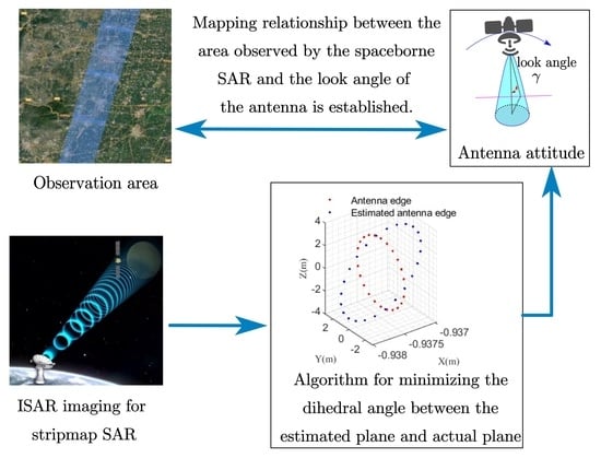
- One-to-one correspondence is established between the time-varying area observed by the spaceborne SAR operating in boresight stripmap mode and the look angle of the spaceborne SAR’s antenna, which provides a new approach to estimating the time-varying area observed by spaceborne SARs operating in boresight stripmap mode.
- (2)
- According to the ISAR imaging model for spaceborne SAR, a concise expression of the ISAR projection matrix is obtained via matrix derivation.
- (3)
- The proposed algorithm has no special constraints on the antenna structure of the spaceborne SAR, and is only based on the coplanarity of the scatterers on the parabolic antenna edge or the panel antenna of the spaceborne SAR. In addition, an objective function to estimate the look angle of the spaceborne SAR operating in boresight stripmap mode is established, according to the principle of minimizing the dihedral angle between the plane containing the ideal estimated scatterers and the plane containing the actual parabolic antenna edge.
- (4)
- Based on the coplanarity of the scatterers on the parabolic antenna edge of a spaceborne SAR, it is easy to obtain an accurate normal vector of the antenna edge datum plane. In addition, using the dihedral angle to construct the objective function, the characteristic is obvious, the performance is stable, and the algorithm has good robustness.
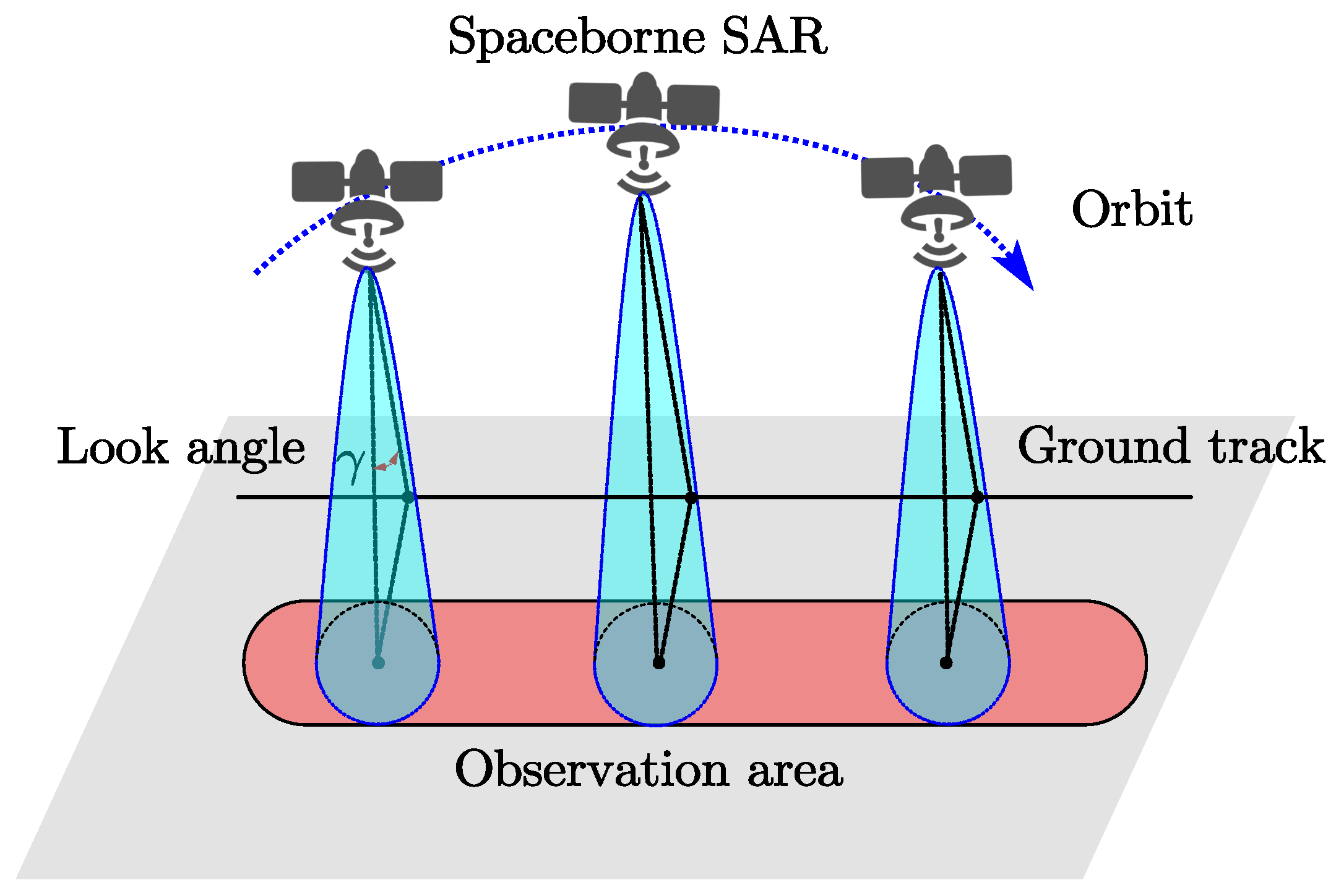
2. Geometry of Stripmap SAR Observation
2.1. Characteristics of Stripmap SAR
2.2. Model of the Stripmap SAR Observation Area
3. ISAR Imaging and Method for Estimating the Stripmap SAR Observation Area
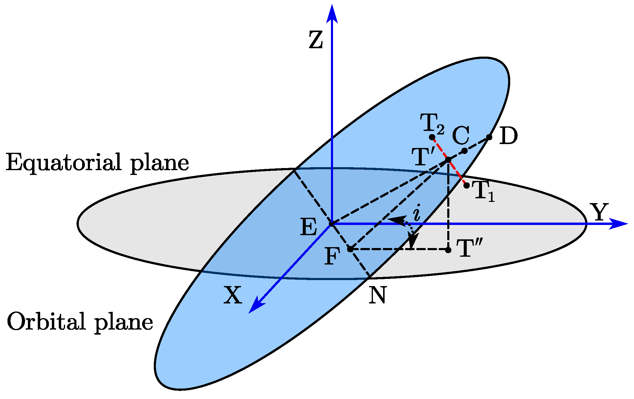
3.1. Coordinate Systems
- (1)
- Component body coordinates (CB): . The component coordinate system and the satellite component are fixedly connected. When the satellite component is not moving, the component body coordinates and the satellite body coordinates coincide with each other. When the spaceborne SAR operating in boresight stripmap mode observes the Earth, it is rotated around the Y-axis to obtain the satellite body coordinates. This coordinate system is used to describe the satellite component attitude relative to the satellite body.
- (2)
- ISAR imaging coordinates system (IMG): . The origin O is the centroid of the space target, the positive X-axis is the same as the radar line-of-sight, the positive Z-axis is the same as the direction of the effective rotation vector of the space target, and the Y-axis and the X- and Z-axes form a right-handed Cartesian coordinate system. This coordinate system is used to describe the variations in the scatterers on the space target relative to the ISAR imaging plane.
- (3)
- Geocentric orbit reference coordinates (REF): . The origin E is the geocenter, the positive X-axis is the direction from the geocenter to the space target centroid at the zenith when the ground-based radar observes the space target, the Y-axis is in the orbital plane and perpendicular to the X-axis along the direction of tangential velocity, and the Z-axis, X-axis, and Y-axis form a Cartesian right-handed coordinate system. This coordinate system is used to describe the space target position.
3.2. ISAR Imaging Principle and Model
3.2.1. ISAR Imaging Principle
3.2.2. ISAR Imaging Model for Spaceborne SAR
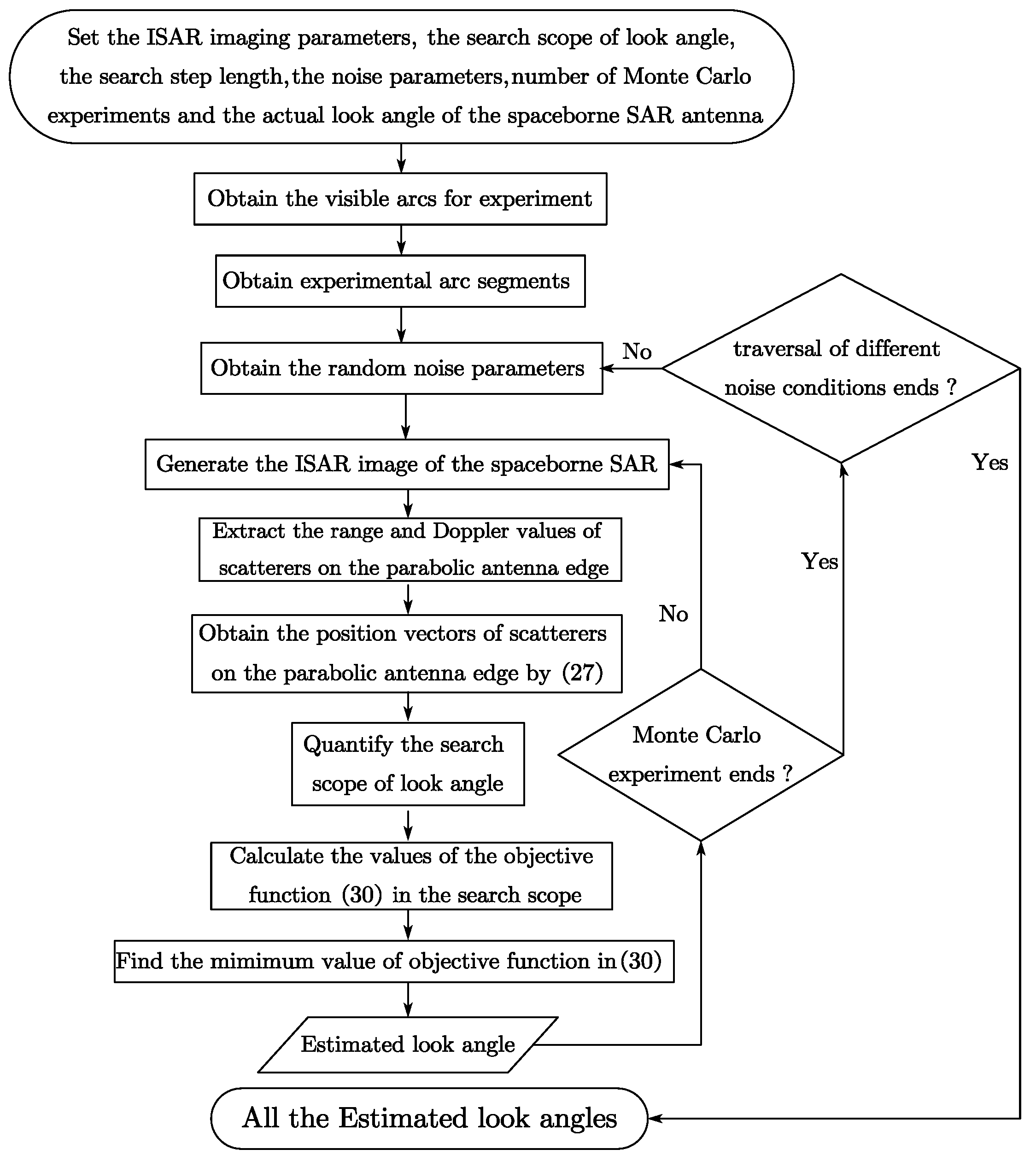
3.3. Method for Estimating the Stripmap SAR Observation Area
4. Simulation Experiments
4.1. Experimental Data Generation
4.2. Feasibility Verification Experimental Methodology
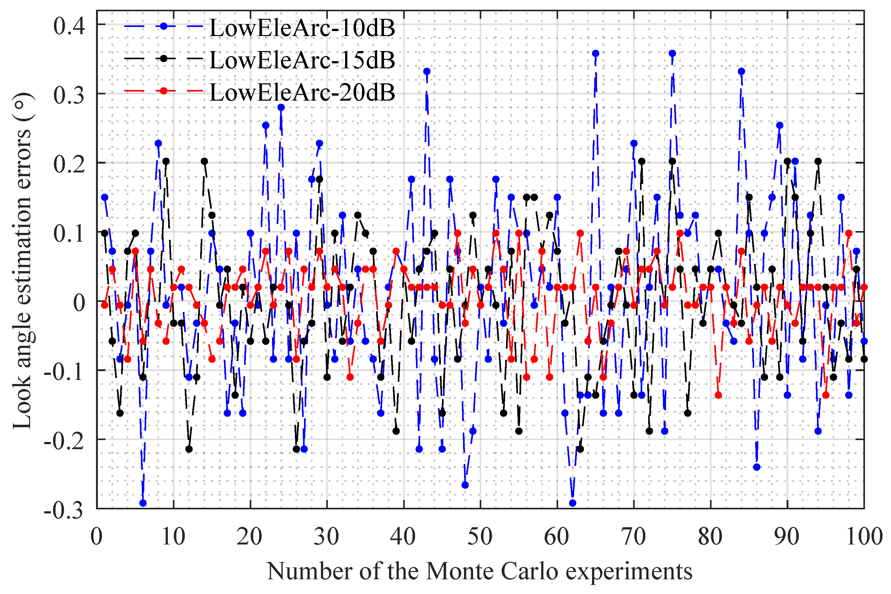
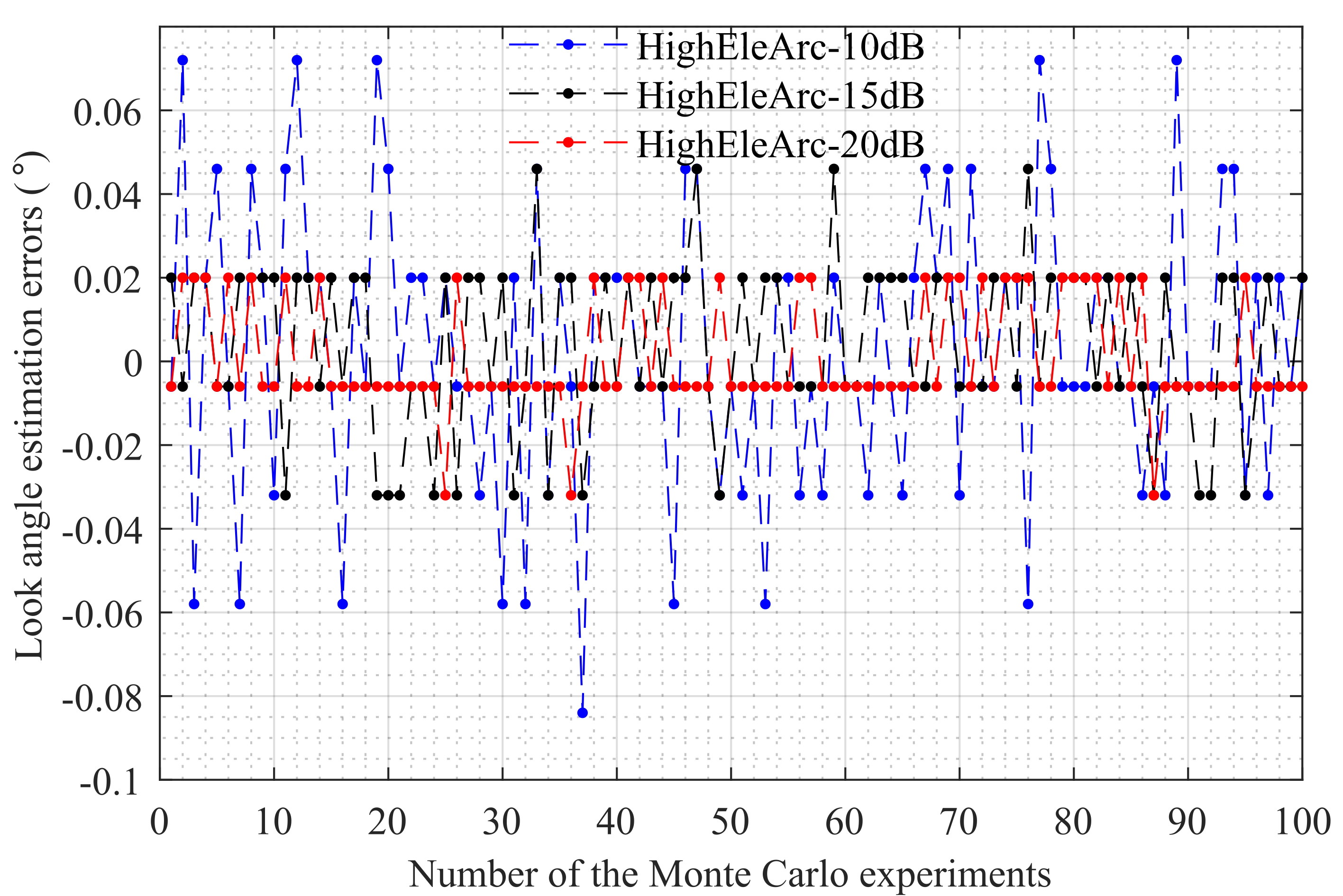
4.3. Robustness Validation Experimental Methodology
5. Experimental Results and Analysis
5.1. Feasibility Results and Analysis of the Algorithm for Minimizing the Dihedral Angle between the Estimated Plane and Actual Plane
5.2. Robustness Results and Analysis of the Algorithm for Minimizing the Dihedral Angle between the Estimated Plane and Actual Plane
6. Conclusions
Author Contributions
Funding
Data Availability Statement
Acknowledgments
Conflicts of Interest
Abbreviations
| SAR | Synthetic aperture radar |
| ISAR | Inverse synthetic aperture radar |
| TIRA | Tracking and imaging radar |
| SFM | Structure from motion |
| SVD | Singular value decomposition |
| InSAR | Interferometric synthetic aperture radar |
| SNR | Signal-to-noise ratio |
References
- Moreira, A.; Prats-Iraola, P.; Younis, M.; Krieger, G.; Hajnsek, I.; Papathanassiou, K.P. A tutorial on synthetic aperture radar. IEEE Geosci. Remote Sens. Mag. 2013, 1, 6–43. [Google Scholar] [CrossRef]
- Franceschetti, G.; Lanari, R. Synthetic Aperture Radar Processing; CRC Press: Boca Raton, FL, USA, 1999. [Google Scholar]
- Ozdemir, C. Inverse Synthetic Aperture Radar Imaging with MATLAB Algorithms; John Wiley & Sons: Hoboken, NJ, USA, 2021. [Google Scholar]
- Ma, Y.; Soatto, S.; Košecká, J.; Sastry, S. An Invitation to 3-d Vision: From Images to Geometric Models; Springer: Berlin/Heidelberg, Germany, 2004; Volume 26. [Google Scholar]
- Hartley, R.; Zisserman, A. Multiple View Geometry in Computer Vision; Cambridge University Press: Cambridge, UK, 2003. [Google Scholar]
- Liu, L.; Zhou, F.; Bai, X.R.; Tao, M.L.; Zhang, Z.J. Joint cross-range scaling and 3D geometry reconstruction of ISAR targets based on factorization method. IEEE Trans. Image Process. 2016, 25, 1740–1750. [Google Scholar] [CrossRef] [PubMed]
- Tomasi, C.; Kanade, T. Shape and motion from image streams: A factorization method. Proc. Natl. Acad. Sci. USA 1993, 90, 9795–9802. [Google Scholar] [CrossRef] [PubMed]
- Morita, T.; Kanade, T. A sequential factorization method for recovering shape and motion from image streams. IEEE Trans. Pattern Anal. Mach. Intell. 1997, 19, 858–867. [Google Scholar] [CrossRef]
- Rong, J.; Wang, Y.; Han, T. Interferometric ISAR imaging of maneuvering targets with arbitrary three-antenna configuration. IEEE Trans. Geosci. Remote Sens. 2019, 58, 1102–1119. [Google Scholar] [CrossRef]
- Zhao, L.; Gao, M.; Martorella, M.; Stagliano, D. Bistatic three-dimensional interferometric ISAR image reconstruction. IEEE Trans. Aerosp. Electron. Syst. 2015, 51, 951–961. [Google Scholar] [CrossRef]
- Zhou, Y.; Zhang, L.; Wang, H.; Qiao, Z.; Hu, M. Attitude estimation of space targets by extracting line features from ISAR image sequences. In Proceedings of the 2017 IEEE International Conference on Signal Processing, Communications and Computing (ICSPCC), Xiamen, China, 22–25 October 2017; pp. 1–4. [Google Scholar]
- Duan, J.; Xie, P.; Zhang, L.; Ma, Y. Space target dynamic identification by exploiting geometrical feature flow from ISAR image sequences. IEEE Sens. J. 2022, 22, 21877–21884. [Google Scholar] [CrossRef]
- Xie, P.; Zhang, L.; Du, C.; Wang, X.; Zhong, W. Space target attitude estimation from ISAR image sequences with key point extraction network. IEEE Signal Process. Lett. 2021, 28, 1041–1045. [Google Scholar] [CrossRef]
- Zhou, Y.; Zhang, L.; Cao, Y.; Wu, Z. Attitude estimation and geometry reconstruction of satellite targets based on ISAR image sequence interpretation. IEEE Trans. Aerosp. Electron. Syst. 2018, 55, 1698–1711. [Google Scholar] [CrossRef]
- Wang, J.; Li, Y.; Song, M.; Xing, M. Joint estimation of absolute attitude and size for satellite targets based on multi-feature fusion of single ISAR image. IEEE Trans. Geosci. Remote Sens. 2022, 60, 1–20. [Google Scholar] [CrossRef]
- Wang, J.; Du, L.; Li, Y.; Lyu, G.; Chen, B. Attitude and size estimation of satellite targets based on ISAR image interpretation. IEEE Trans. Geosci. Remote Sens. 2021, 60, 1–15. [Google Scholar] [CrossRef]
- Afshar, R.; Lu, S. Classification and recognition of space debris and its pose estimation based on deep learning of CNNs. In Proceedings of the HCI International 2020-Posters: 22nd International Conference, HCII 2020, Copenhagen, Denmark, 19–24 July 2020; Proceedings, Part I 22. Springer: Berlin/Heidelberg, Germany, 2020; pp. 605–613. [Google Scholar]
- Arakawa, R.; Matsushita, Y.; Hanada, T.; Yoshimura, Y.; Nagasaki, S. Attitude estimation of space objects using imaging observations and deep learning. In Proceedings of the Advanced Maui Optical and Space Surveillance Technologies Conference, Maui, HI, USA, 17–20 September 2019; p. 21. [Google Scholar]
- Bovik, A.C. Handbook of Image and Video Processing; Academic Press: Cambridge, MA, USA, 2010. [Google Scholar]
- Cumming, I.; Wong, F. Digital Processing of Synthetic Aperture Radar Data: Algorithms and Implementation; Artech House: Norwood, MA, USA, 2005. [Google Scholar]
- Markley, F.; Crassidis, J. Fundamentals of Spacecraft Attitude Determination and Control; Springer: New York, NY, USA, 2014. [Google Scholar]
- Vallado, D.A. Fundamentals of Astrodynamics and Applications; Springer Science & Business Media: Berlin/Heidelberg, Germany, 2001; Volume 12. [Google Scholar]
- Li, G.; Liu, Y.; Wu, L.; Xu, S.; Chen, Z. Three-dimensional reconstruction using ISAR sequences. In Proceedings of the MIPPR 2013: Pattern Recognition and Computer Vision, Wuhan, China, 26–27 October 2013; Volume 8919, pp. 43–49. [Google Scholar]
- Wang, F.; Eibert, T.F.; Jin, Y.Q. Simulation of ISAR imaging for a space target and reconstruction under sparse sampling via compressed sensing. IEEE Trans. Geosci. Remote Sens. 2015, 53, 3432–3441. [Google Scholar] [CrossRef]
- Zhang, Y.; Yang, X.; Jiang, X.R.; Yang, Q.; Deng, B.; Wang, H.Q. Attitude direction estimation of space target parabolic antenna loads using sequential terahertz ISAR images. J. Infrared Millim. Waves 2021, 40, 497–507. [Google Scholar]
- Wertz, J.R. Spacecraft Attitude Determination and Control; Springer Science & Business Media: Berlin/Heidelberg, Germany, 2012; Volume 73. [Google Scholar]
- Shaviv, G.; Shachar, M. TechSAT-1–an earth-pointing, three-axis stabilized microsatellite. Space Technol. 1995, 4, 245–256. [Google Scholar] [CrossRef]
- Sun, G.C.; Liu, Y.; Xiang, J.; Liu, W.; Xing, M.; Chen, J. Spaceborne synthetic aperture radar imaging algorithms: An overview. IEEE Geosci. Remote Sens. Mag. 2021, 10, 161–184. [Google Scholar] [CrossRef]
- Iwata, T.; Yoshizawa, T.; Hoshino, H.; Maeda, K. Precision attitude and orbit control system for the advanced land observing satellite. In Proceedings of the AIAA Guidance, Navigation, and Control Conference and Exhibit, Austin, TX, USA, 11–14 August 2003; p. 5783. [Google Scholar]
- Lee, S.; Park, S.Y.; Kim, J.; Ka, M.H.; Song, Y. Mission Design and Orbit-Attitude Control Algorithms Development of Multistatic SAR Satellites for Very-High-Resolution Stripmap Imaging. Aerospace 2022, 10, 33. [Google Scholar] [CrossRef]


| Orbital Elements | Values |
|---|---|
| Semimajor axis | 6946.615 km |
| Eccentricity | 0.00048 |
| Inclination | 36.93 |
| Right ascension of ascending node | 334.87 |
| Argument of perigee | 63.81 |
| True anomaly | 296.05 |
| Epoch time | 22,191.71487269 |
| Radar Parameters | Values |
|---|---|
| Waveform | LFM |
| Center frequency | 16.8 GHz |
| Bandwidth | 1 GHz |
| Pulse repetition frequency | 50 Hz |
| Sampling frequency | 1.5 GHz |
| Image resolution cells | 15 × 15 cm |
| Location Parameters | Values |
|---|---|
| Latitude | 41 N |
| Longitude | 86.8 E |
| Altitude | 0 km |
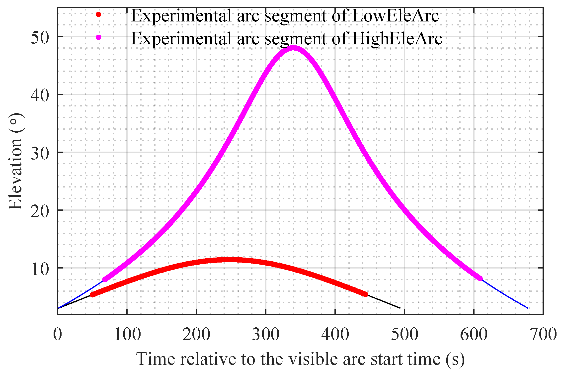
| Visible Arcs | Duration (s) | Maximum Elevation Angle () |
|---|---|---|
| Arc-1 | 501 | 11.70 |
| Arc-2 | 654 | 31.94 |
| Arc-3 | 681 | 48.50 |
| Arc-4 | 662 | 35.20 |
| Arc-5 | 539 | 14.04 |
| Arc Segment | SNR | ||
|---|---|---|---|
| LowEleArc | 10 dB | 0.0156° | 0.1487° |
| 15 dB | 0.0026° | 0.1063° | |
| 20 dB | 0.0057° | 0.0545° | |
| HighEleArc | 10 dB | 0.0031° | 0.0337° |
| 15 dB | 0.0041° | 0.0202° | |
| 20 dB | 0.0008° | 0.0131° |
Disclaimer/Publisher’s Note: The statements, opinions and data contained in all publications are solely those of the individual author(s) and contributor(s) and not of MDPI and/or the editor(s). MDPI and/or the editor(s) disclaim responsibility for any injury to people or property resulting from any ideas, methods, instructions or products referred to in the content. |
© 2023 by the authors. Licensee MDPI, Basel, Switzerland. This article is an open access article distributed under the terms and conditions of the Creative Commons Attribution (CC BY) license (https://creativecommons.org/licenses/by/4.0/).
Share and Cite
Li, B.; Chen, D.; Cao, H.; Wang, J.; Li, H.; Fu, T.; Zhang, S.; Zhao, L. Estimating the Observation Area of a Stripmap SAR via an ISAR Image Sequence. Remote Sens. 2023, 15, 5484. https://doi.org/10.3390/rs15235484
Li B, Chen D, Cao H, Wang J, Li H, Fu T, Zhang S, Zhao L. Estimating the Observation Area of a Stripmap SAR via an ISAR Image Sequence. Remote Sensing. 2023; 15(23):5484. https://doi.org/10.3390/rs15235484
Chicago/Turabian StyleLi, Bo, Defeng Chen, Huawei Cao, Junling Wang, Haiguang Li, Tuo Fu, Shuo Zhang, and Lizhi Zhao. 2023. "Estimating the Observation Area of a Stripmap SAR via an ISAR Image Sequence" Remote Sensing 15, no. 23: 5484. https://doi.org/10.3390/rs15235484
APA StyleLi, B., Chen, D., Cao, H., Wang, J., Li, H., Fu, T., Zhang, S., & Zhao, L. (2023). Estimating the Observation Area of a Stripmap SAR via an ISAR Image Sequence. Remote Sensing, 15(23), 5484. https://doi.org/10.3390/rs15235484