Article

Wheat Yield Prediction Using Unmanned Aerial Vehicle RGB-Imagery-Based Convolutional Neural Network and Limited Training Samples

1
College of Water Resources and Civil Engineering, China Agricultural University, Beijing 100083, China
2
Institute of Environment and Sustainable Development in Agriculture, Chinese Academy of Agricultural Sciences, Beijing 100081, China
3
Dryland Farming Institute, Hebei Academy of Agriculture and Forestry Sciences, Hengshui 053000, China
4
Key Laboratory of Crop Drouht Tolerance Research of Heibei Province, Hengshui 053000, China
*
Author to whom correspondence should be addressed.
These authors contributed equally to this work.
Remote Sens. 2023, 15(23), 5444; https://doi.org/10.3390/rs15235444
Submission received: 26 September 2023 / Revised: 1 November 2023 / Accepted: 8 November 2023 / Published: 21 November 2023
(This article belongs to the Section Remote Sensing in Agriculture and Vegetation)

Abstract

:
Low-cost UAV RGB imagery combined with deep learning models has demonstrated the potential for the development of a feasible tool for field-scale yield prediction. However, collecting sufficient labeled training samples at the field scale remains a considerable challenge, significantly limiting the practical use. In this study, a split-merge framework was proposed to address the issue of limited training samples at the field scale. Based on the split-merge framework, a yield prediction method for winter wheat using the state-of-the-art Efficientnetv2_s (Efficientnetv2_s_spw) and UAV RGB imagery was presented. In order to demonstrate the effectiveness of the split-merge framework, in this study, Efficientnetv2_s_pw was built by directly feeding the plot images to Efficientnetv2_s. The results indicated that the proposed split-merge framework effectively enlarged the training samples, thus enabling improved yield prediction performance. Efficientnetv2_s_spw performed best at the grain-filling stage, with a coefficient of determination of 0.6341 and a mean absolute percentage error of 7.43%. The proposed split-merge framework improved the model ability to extract indicative image features, partially mitigating the saturation issues. Efficientnetv2_s_spw demonstrated excellent adaptability across the water treatments and was recommended at the grain-filling stage. Increasing the ground resolution of input images may further improve the estimation performance. Alternatively, improved performance may be achieved by incorporating additional data sources, such as the canopy height model (CHM). This study indicates that Efficientnetv2_s_spw is a promising tool for field-scale yield prediction of winter wheat, providing a practical solution to field-specific crop management.

1. Introduction

Yield prediction is vital in wheat breeding, precise field management, and decision making [1,2,3,4,5,6]. Field-scale wheat yields can be influenced by many factors, such as genotypes, soil conditions, stress, environments, and field management practices [2,3,7,8]. The sensitivity to these factors varies between cultivars, regions, site conditions, and growth stages [9,10], which causes varying levels of impact on the yield. Therefore, timely and accurate wheat yield prediction at the field scale can help field-specific management be performed [4,11,12,13,14,15,16].
Recently, adopting machine learning (ML) models in conjunction with images of high spatiotemporal resolution captured by unmanned aerial vehicles (UAVs) is the dominant approach for field-scale crop yield prediction [1,9,11,17,18,19]. Many yield prediction studies followed the pipelined procedures of canopy feature extraction and selection and ML model construction [1,9,11,12,20,21,22], proposing the feature-based method, wherein feature selection is essential to the feature-based method [5,9,13,23,24], which aims to select the most relevant features for yield prediction. However, selecting features robust to the variability in field conditions can be challenging since winter wheat canopies are prone to vary due to the changes in environments and field practices [13,25]. In addition, this task is subject to one’s expert domain knowledge [9,13,26]. Consequently, the feature-based method tends to have weak generalization ability.
In order to generalize the yield prediction methods to as much variability as possible in field conditions, the feature selection process should be capable of adaptively selecting features representing the crop canopy. It is reported that convolutional neural networks (CNNs) can perform automatic feature learning from input data [27,28], making it a powerful tool for image analysis. Therefore, studies also adopt CNNs for field-scale crop yield prediction, proposing the imagery-based prediction method [6,8,26,29,30]. UAV-based RGB [8,29,30] and multispectral [6,8,26,30] imagery are the two main image types for imagery-based yield prediction. Although the RGB imagery contains less canopy spectral information than the multispectral imagery, it has better ground resolution and, therefore, more informative canopy spatial features [16,19]. Consequently, CNNs with RGB imagery are not necessarily inferior to those with multispectral imagery on field-scale yield prediction [6,26,29]. In addition, since RGB imagery has only three channels, i.e., red, green, and blue, the processing of the RGB imagery does not require complicated calibrations, for example, radiometric calibration, making it fast and convenient to generate the orthomosaic maps [31,32]. Given the low cost of image collection and the inherent characteristics, UAV RGB-imagery-based CNNs are a promising tool for yield prediction in field conditions. Nevavuori et al. [29] used a simple CNN (containing six convolutional layers) and RGB imagery to predict crop yields, which achieved the best MAPE score of 8.8%. Similarly, the CNN in Yang et al. [30] was also simple (five convolutional layers for the RGB branch), achieving the best MAPE score of 26.61%. The above studies highlight the potential of RGB-imagery-based CNNs in crop yield prediction. However, the influencing factors in field conditions are diverse, making field-scale yield prediction a challenging task that cannot be achieved by using a simple CNN. Consequently, more studies are still needed to improve prediction accuracy by adopting the appropriate networks. Compared with the networks in the above studies [6,26,29,30], the recent state-of-the-art networks tend to have more parameters and deepened network depth, requiring massive training samples. However, collecting sufficient labeled samples at the field scale is challenging [4,13,29,33,34]. Therefore, a practical solution to achieve accurate yield prediction with limited labeled samples should be explored.
Motivated by the issue of limited training samples at the field scale, this study proposed a split-merge framework, which was dedicated to enlarging the training samples. Based on the split-merge framework, a field-scale yield prediction method for winter wheat using the RGB-imagery-based CNN and limited training samples was proposed. The split-merge framework first split the canopy images into sub-images, based on which the construction of the RGB-imagery-based CNN was achieved. Next, the results of the sub-images were merged to obtain the results of the corresponding canopy images. The main objectives of this study were (1) to investigate if the split-merge framework could improve the yield prediction performance under the circumstance of limited training samples, (2) to test whether the proposed yield prediction method can adapt to different irrigation regimes, and (3) to explore the optimal growth stage for yield prediction of winter wheat using the proposed method. The proposed method is expected to achieve accurate wheat yield predictions using low-cost UAV RGB imagery at the field scale and support site-specific field management.

2. Materials and Methods

2.1. Experimental Setup

The experiments were conducted on an experimental field belonging to the Field station of Dryland Farming Institute, Hebei Academy of Agriculture and Forestry Sciences, Hengshui, China (Figure 1a, Lat: 37°54′15.63″N, Long: 115°42′29.32″E). The station is in the temperate continental monsoon climate zone, and the primary soil type is fluvo-aquic soil. The annual average temperature and precipitation are 13.3 °C and 497.1 mm, respectively. During the 2020–2021 growing season, a total precipitation of 43.9 mm was received [21]. The experimental field was approximately 20 m in width and 165m in length, covering a total area of 0.3 ha (Figure 1b). The experiment adopted 11 winter wheat cultivars, i.e., Chang8744, Shimai22, Luyuan47, Shimai15, HengH160, Xinmai28, Jimai41, Shannong28, Nongda212, Heng4399, and Jimai22, which were planted with seven water treatments, including one well-watered treatment (F), one rainfed treatment (N), and five deficit water treatments (D1 to D5). Notably, in order to avoid the influence of the water treatments during irrigation, this study used plastics buried into the ground to a depth of 1.2 m to separate the treatments from each other. Each treatment was applied to three replicates. Accordingly, a total of 231 plots were established, and the size of each plot was 1.5 m × 6 m. Details on the irrigation time and amount are shown in Table 1. The experiment used 750 kg ha−1 of 1:1:1 (15% N, 15% P2O5, 15% K2O) fertilizer, which was applied to the experimental field before sowing. Diseases, insects, and weeds were managed according to the local practice. All the treatments were sown on 15 October 2020, while the harvest date varied according to the winter wheat growth. Specifically, the well-watered treatment was harvested on 11 June 2021, and the other treatments were harvested on 8 June 2021.

2.2. Data Acquisition

2.2.1. Field Data Collection

Destructive sampling was used to measure the wheat grain yield (kg ha−1). For each plot, winter wheat plants covering an area of 3.24 m2 were collected (six rows, each with a length of 3 m and a row space of 0.18 m), based on which the plot-wise wheat grain yield was obtained at a 13% moisture level according to the following calculations.
Y i = y i × 1 m i / 0.87 3.24 × 10000 1000  
where Y i , y i , and m i were the plot-wise wheat grain yield (kg), the sample wheat grain yield (g), and the wheat grain moisture of the i t h plot, respectively. This study used a mini-GAC plus (DICKEY-john, Minneapolis, MN, USA) to measure the wheat grain moisture.

2.2.2. UAV RGB Imagery Collection

The camera for RGB imagery collection was a Zenmuse XT2 camera (DJI Technology Co., Ltd., Shenzhen, China), which has a 1/1.7″ CMOS image sensor with a field of view of 57.12° × 42.44°, thus capturing images of 4000 × 3000-pixel resolution. A drone of DJI M200 (DJI Technology Co., Ltd., Shenzhen, China) with a single gimbal was used to carry the camera. A total of five flights were conducted at an interval of approximately ten days during the experiment, covering the growth stages from jointing to grain-filling. The specific date and the corresponding Zadoks [35] growth stages (GSs) are shown in Table 2. Image collection was conducted under clear-sky conditions. During the flying campaigns, the UAV flew at an altitude of 50 m and a speed of 1.7 m/s. The forward and side overlaps were 80% and 70%, respectively. Twelve ground control points (GCPs) were set up in the experimental field (Figure 1b) using waterproof black marks on the irrigation pipe made of white polyvinyl chloride. The locations of the irrigation pipe were along both sides of the experimental field and remained fixed during the experiment. The dimensions of the GCP were about 10 cm × 10 cm. A handheld BHCNAV LT500 GPS (Huace Navigation Technology Ltd., Shanghai, China) was used to measure the precise geographic coordinates of each GCP.

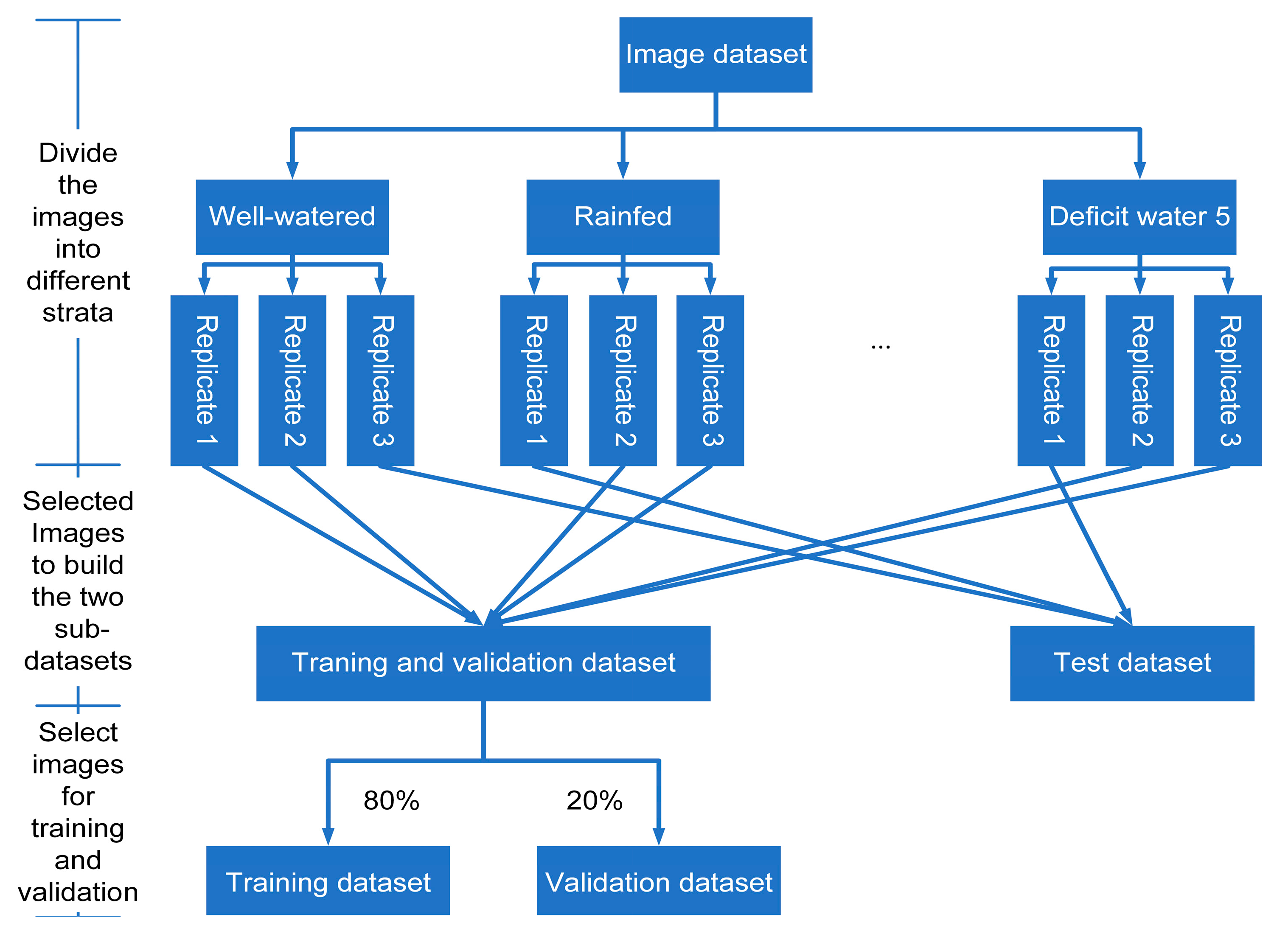
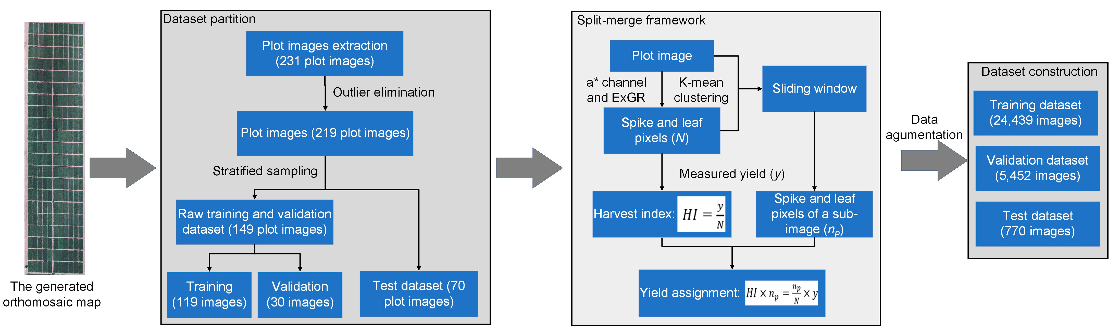
2.2.3. Data Preprocessing

The orthomosaic maps were generated using the Agisoft Metashape v1.7 (Agisoft LLC, St. Petersburg, Russia). In order to build high-quality orthomosaic maps, this study used the geographic coordinates of the GCPs during the workflow for geo-reference. According to the camera and the flying parameters, orthomosaic maps with a ground resolution of around 1.2 cm could be generated. In order to keep the consistency for all orthomosaic maps and avoid the errors caused by the inconsistent pixel size of a plot image in different orthomosaic maps, this study uniformly adjusted the ground resolution of all orthomosaic maps to 1.3 cm.
In order to construct the yield prediction model, plot images were extracted from the orthomosaic maps to build the image dataset. Notably, the plots at the right end of the orthomosaic map did not belong to the experiment of this study (Figure 1b) and were eliminated. Next, outlier elimination was conducted according to the harvest index (HI), which was cultivar-dependent [34] and calculated as the ratio between the grain yield and the above-ground biomass. Specifically, if a plot yield value obviously deviated from the two replicates while the corresponding above-ground biomass value was consistent with the two replicates, it would be considered an outlier. After the outlier elimination, two sub-datasets were built through stratified sampling (Figure 2), i.e., the training and validation dataset and the test dataset. Specifically, the image dataset was first divided into different strata according to the water treatment and the replicate. Next, images were proportionally selected from the different strata to build the two sub-datasets. Notably, the ratio of the training and validation to test stood at 2:1. Consequently, the training and validation dataset was composed of 149 images, and the test dataset was composed of 70 images. Moreover, this study further divided the training and validation dataset into a training dataset comprising 119 images and a validation dataset comprising 30 images.

2.3. The Field-Scale Yield Prediction Method

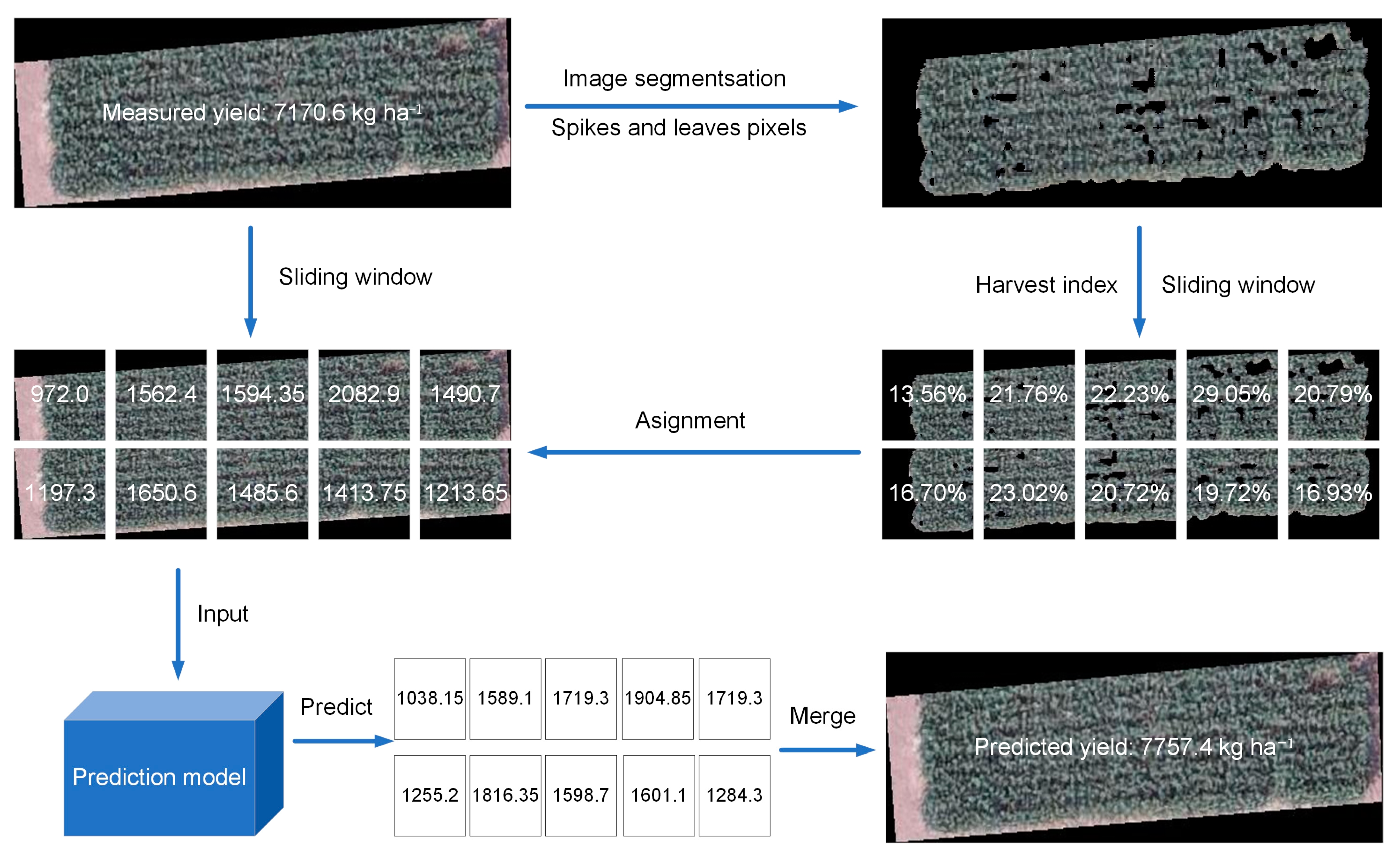
2.3.1. The Split-Merge Framework

In this study, the number of training samples was severely insufficient for training a CNN. Even if data augmentation strategies were used, more training images would still be needed to meet the data demand. To ensure adequate training of the CNNs, this study proposed the split-merge framework to enlarge the training samples. The split-merge framework consisted of two stages (Figure 3), i.e., the split and the merge stages. The split stage aimed to split each canopy image into sub-images using a sliding window. Given the pixel resolution of the plot images, this study adopted a sliding window of 112 × 112-pixel resolution and multiple stride values, aiming to diversify the training samples. In order to achieve the number-of-samples/accuracy trade-off and to retain a reasonable number of training images for limited computing resources, the stride values were 24, 34, 44, 50, 61, 74, 87, 103, and 112. Notably, if a canopy image could not be sampled into 112 × 112 sub-images, due to the mismatch between the image size and a stride value, this study would reduce the stride value at the edges to make the sliding window fit the size of the canopy image. Multiple stride values were only applied to the training and the validation datasets. Unlike the training and the validation datasets, the canopy images in the test dataset were sampled by a sliding window with a stride value of 112 pixels. Based on the above strategies, the training dataset was enlarged to 24,439, and the validation dataset was enlarged to 5452.
An essential part of the split-merge framework was to assign a yield value to the sub-images. This study achieved the yield assignment of sub-images based on the HI. Previous studies [34,36,37] have shown that the number of spike and leaf pixels in a canopy image could represent the above-ground biomass and was, therefore, proportional to the yield. Accordingly, the number of spike and leaf pixels of a sub-image was proportional to the corresponding yield value, which could transfer the yield assignment to the segmentation of spike and leaf pixels. This study used the k-means cluster algorithm with an a* channel of the CIELa*b* color space and excess green minus excess red (ExGR) [38] to segment the spike and leaf pixels. Once the segmentation of spike and leaf pixels of a plot image was completed, the HI could be calculated using (1), and the yield assignment of a sub-image could be obtained using (2). The pipeline procedures for image preprocessing in this study are shown in Figure 4.
H I = y N
y p = H I × n p = n p N × y
where y and N are the wheat grain yield and the number of spike and leaf pixels of a plot image, respectively. n p is the number of spike and leaf pixels of the sub-images and y p is the assigned yield value. The merge stage aimed to merge the prediction results of sub-images to obtain the yield predictions. The values at the overlapping regions were calculated through averaging.

2.3.2. The RGB-Imagery-Based Yield Prediction Model

According to the experimental design, the yield prediction models learned to map images to yield values, which proved feasible in previous studies [27,28]. Unlike the previous studies by Nevavuori et al. [29] and Yang et al. [30], this study chose to adopt the state-of-the-art CNNs rather than propose custom ones to build the yield prediction model since these models have been proven to be powerful in extracting image features. In addition, these models could use the pre-trained weights from the ImageNet [39] to speed up the convergence. Since the yield prediction model would be applied in field conditions, expensive CNNs that have a large number of parameters would not be considered. In a previous study on crop yield prediction using imagery-based CNN [26], ResNet18 [40] achieved accurate yield prediction results using multispectral imagery. Therefore, this study adopted ResNet18 to construct the wheat yield prediction model, exploring if it could yield comparable performance using low-cost UAV RGB imagery. The architecture of the ResNet18 is shown in Appendix A, Table A1. Mobilenetv3_large [41] and Efficientnetv2_s [42], which performed well on model accuracy and efficiency, were also adopted, respectively, aiming to gain the balance between the prediction accuracy and the computing resource. The architectures of Efficientnetv2_s and Mobilenetv3_large are shown in Appendix A, Table A2 and Table A3.
Based on the split-merge framework, yield prediction models (termed as Efficientnetv2_s_spw, Mobilenetv3_large_spw, and ResNet18_spw) could be constructed with limited training samples, which were immune to the overfitting issue. Given that the adopted CNNs were initially proposed for classification tasks, this study modified the network structures to adapt to the goal of yield prediction. Notably, the modifications mainly focused on the head block and the output layer of each architecture, indicating that the core blocks remained unchanged. Therefore, the ImageNet pre-trained weights could be used. In the case of over-shrinkage of the feature maps, the convolutional layer in the head block of Mobilenetv3_large and Efficientnetv2_s was changed to one, and Resnet18 adopted a completely new head block. The new head block consisted of a convolutional layer (number of kernels = 64, kernel size = 3, stride = 2), a batch normalization layer, and an ReLU layer. Lastly, a regression output layer was added to the end of each architecture, and ResNet18 and Efficientnetv2_s adopted a dropout layer (rate = 0.5) before the regression output layer.
This study implemented the yield prediction models using the PyTorch deep learning framework and optimized the network weights using the stochastic gradient descent with momentum (SGDM). The initial learning rate was 1 × 10⁻⁵ and dropped every 100 epochs by a factor of 0.5. In favor of model convergence, this study adopted L2 Regularization with a factor of 0.005. The batch size was 200, and the maximum number of epochs for training was 300. In order to test the model performance, the model, which achieved the minimum validation loss during the training process, was adopted for the model test over the test dataset. The image processing task was implemented using MATLAB 2020b (MathWorks Inc., Natick, MA, USA).

2.4. Performance Evaluation

To investigate if the split-merge framework for model construction could improve the yield prediction performance, this study constructed the yield prediction models (termed as Efficientnetv2_s_pw, Mobilenetv3_large_pw, and ResNet18_pw) by directly feeding canopy images to the CNNs. Apparently, image augmentation was essential to avoid overfitting issues. This study adopted different augmentations, including light adjusting by ±10% and ±20%, vertical and horizontal flips, adding gaussian noise, and randomly merging. The random merge aimed to randomly select and average two samples from the training dataset. The random merge operation was repeated 119 and 30 times for the training and the validation datasets, respectively, generating an augmented dataset. In this study, a total of ten augmented datasets were generated based on the random merge. According to the augmentations, this study generated 25 augmented datasets.
To explore whether the irrigation regimes impacted the wheat grain yield, as well as to investigate the performance and adaptability of the proposed yield prediction method across the water treatments, this study used the one-way analysis of variance (ANOVA) with an honest significant difference (HSD) Tukey test (p < 0.05). The IBM SPSS Statistics 25 software (IBM Inc., Armonk, NY, USA) was adopted for the ANOVA. Performance evaluation of prediction models based on the two different pipelines was conducted using the evaluation metrics of coefficient of determination (R2) and mean absolute percentage error (MAPE), whose calculations were as follows.
M A P E = 1 n i = 1 n y i y i ^ y i
where y i represents the measured wheat grain yield and y i ^ represents the predicted wheat grain yield. n is the number of test samples.

3. Results

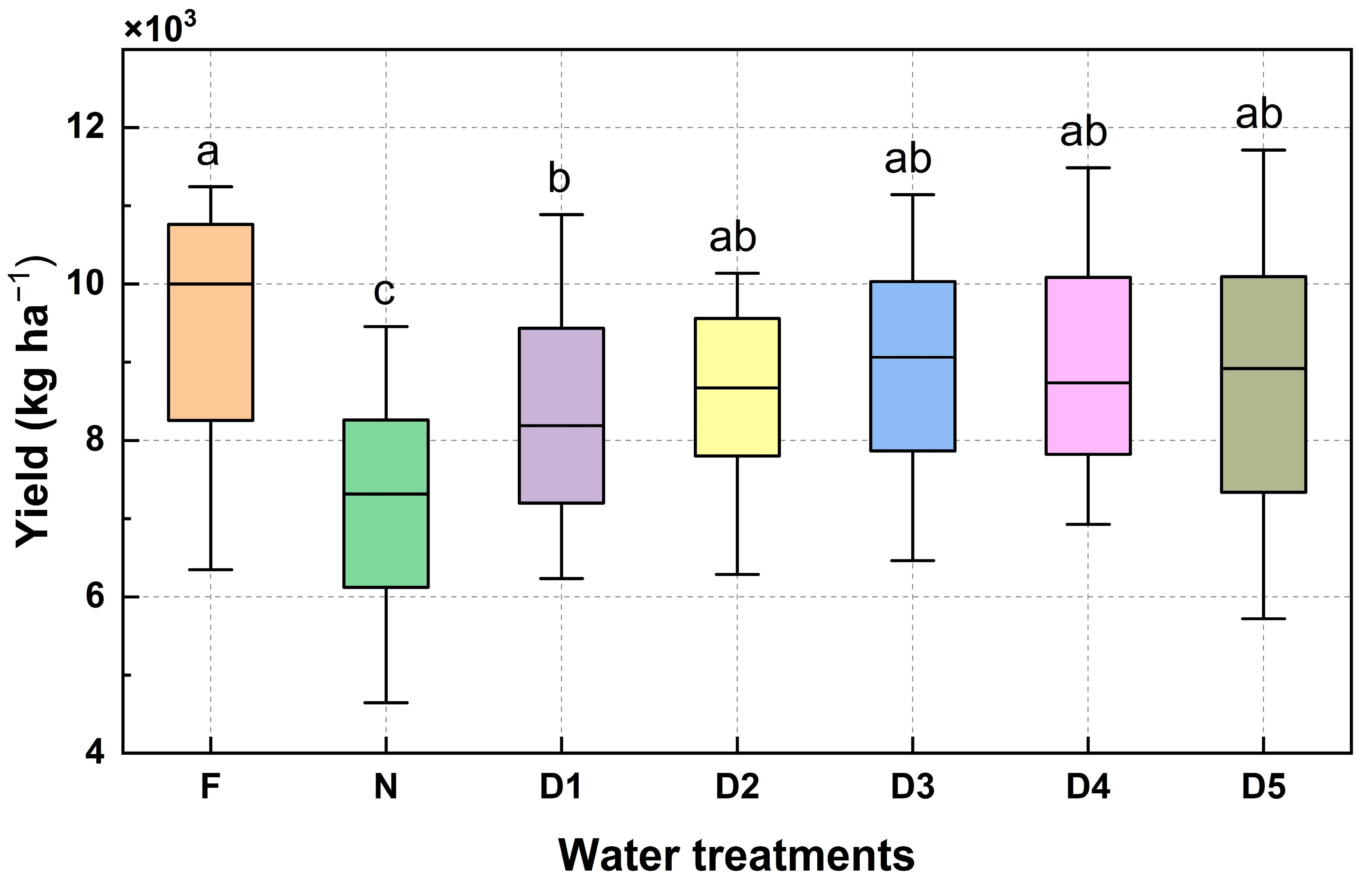
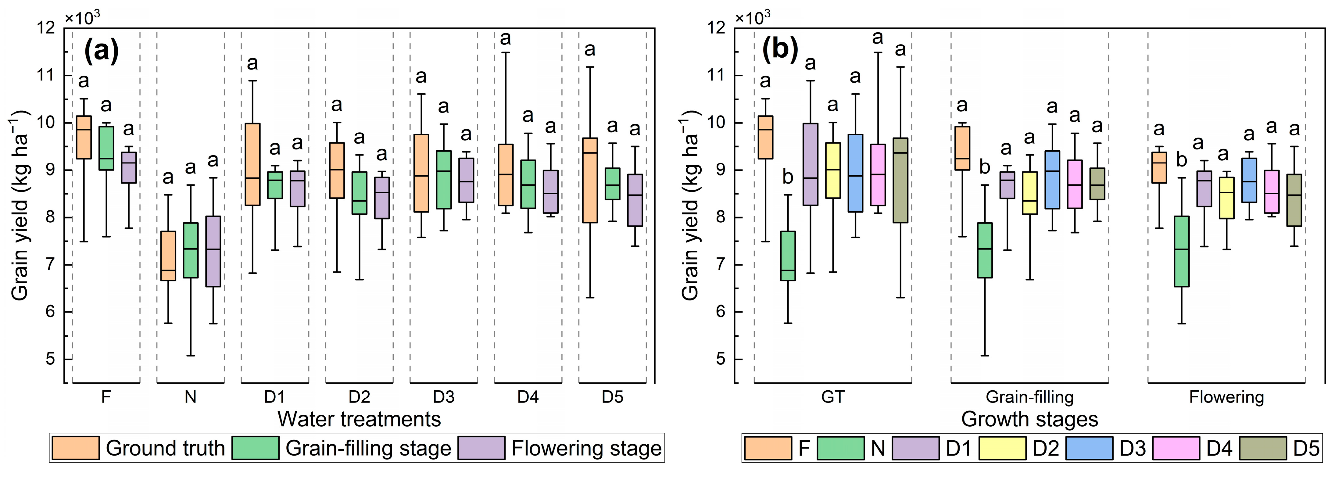
3.1. Impacts of Water Treatments

Grain yield differences across the water treatments are shown in Figure 5. The results indicated significant grain yield differences between the water treatments (p < 0.05). As expected, the well-watered treatment achieved the highest mean yield value (9509.95 kg ha−1), while the rainfed treatment achieved the lowest (7192.52 kg ha−1). The grain yield values among deficit water treatments did not show significant differences, indicating that the time for irrigation would not significantly affect the grain yield of winter wheat. However, it is worth noting that the well-watered treatment achieved a higher mean grain yield than deficit water treatment 1 (8318.62 kg ha−1), suggesting irrigations after over-wintering.

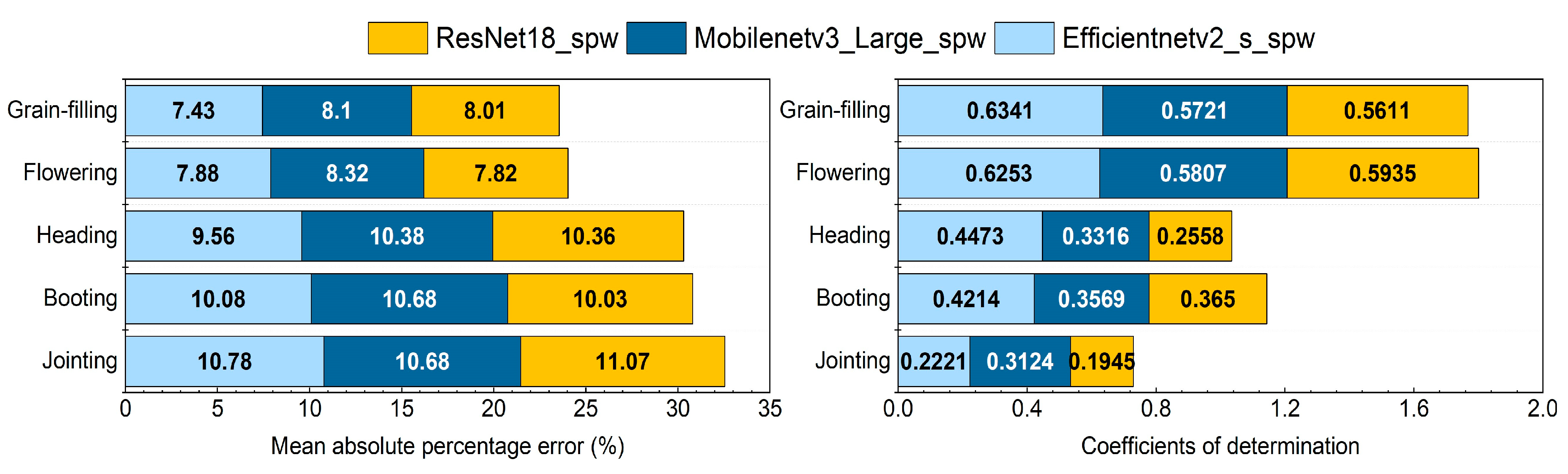
3.2. Prediction Results of the Yield Prediction Models

The results of the yield prediction models based on the split-merge framework are shown in Figure 6. The results showed that all models achieved a consistent trend that model performance improved with the development progress of winter wheat. Among the three models, Efficientnetv2_s_spw achieved the best performance over the test dataset at the graining-filling stage, with an R2 value of 0.6341 and an MAPE value of 7.43%. Regarding the prediction results from the jointing stage to the flowering stage, Efficientnetv2_s_spw consistently outperformed Mobilenetv3_large_spw and ResNet18_spw with the exception of the jointing stage. Mobilenetv3_Large_spw performed best at the jointing stage. From the jointing stage to the booting stage, the performance of Efficientnetv2_s_spw improved obviously, and it continued improving until the grain-filling stage. The performance of Mobilenetv3_large_spw and ResNet18_spw was close over the test dataset. The results showed that the UAV RGB-imagery-based CNNs could accurately predict winter wheat yield at the field scale.
Since Efficientnetv2_s_spw demonstrated excellent prediction capability with low-cost UAV RGB imagery, it was used to investigate the effects of the split-merge framework by comparing with Efficientnetv2_s_pw (Figure 7). It could be seen that Efficientnetv2_s_pw achieved a similar trend to Efficientnetv2_s_spw where model performance improved with the development progress of winter wheat. The best performance of Efficientnetv2_s_pw was achieved at the grain-filling stage, with an R2 value of 0.5415 and an MAPE value of 8.04%. In contrast, the performance of Efficientnetv2_s_pw at the other four growth stages was poor. Compared to Efficientnetv2_s_spw, Efficientnetv2_s_pw consistently presented worse performance from jointing to grain-filling, revealing the superiority of the split-merge framework under the condition of limited training samples. In summary, the results in Figure 6 and Figure 7 showed that Efficientnetv2_s_spw outperformed Efficientnetv2_s_pw from jointing to grain-filling, indicating that the split-merge framework could sufficiently augment the training samples and allowed improved yield prediction performance.

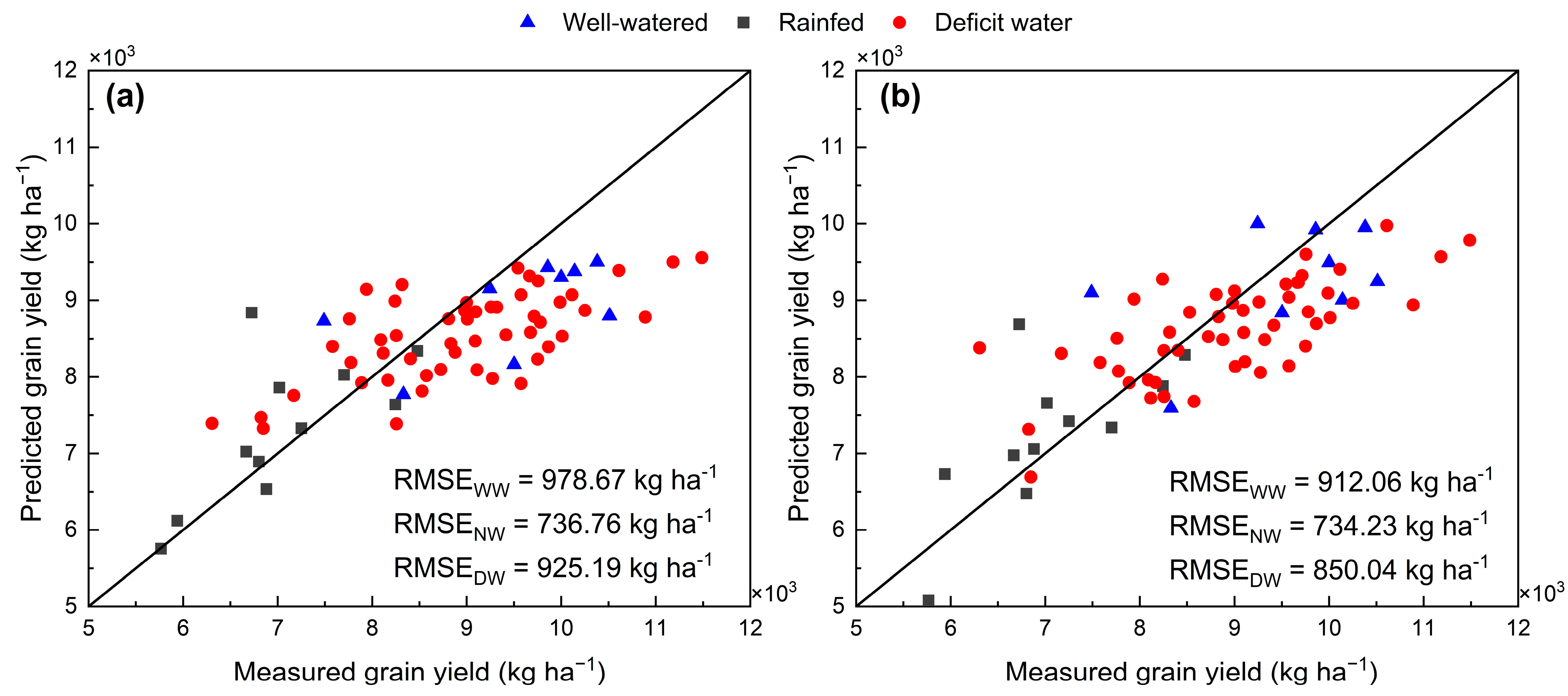
3.3. Performance of the Yield Prediction Model across Water Treatments

This section compares the performance of Efficientnetv2_s_spw across the water treatments. The results (Figure 6) showed that Efficientnetv2_s_spw achieved accurate grain yield predictions at the flowering and grain-filling stages. Therefore, this section mainly focuses on the results at the flowering and grain-filling stages. As shown in Figure 8, there was no significant difference between the ground truth and yield predictions by Efficientnetv2_s_spw across the water treatments (Figure 8a). In addition, predictions by Efficientnetv2_s_spw were consistent with the ground truth (Figure 8b).
The boxplot of the prediction results also revealed that Efficientnetv2_s_spw underestimated the grain yield across the water treatments except for the rainfed treatment (Figure 8a). Especially for the well-watered treatment and deficit water treatments 2–5, Efficientnetv2_s_spw showed more severe underestimations at the flowering stage than at the grain-filling stage. The performance of Efficientnetv2_s_spw across each water treatment is shown in Table 3. It is worth noting that since the difference among the grain yields of the five deficit water treatments was not significant (Figure 5), they were combined as a deficit water treatment for evaluation rather than evaluated separately.
Efficientnetv2_s_spw performed better over the rainfed and the deficit water treatments than the well-watered treatment at both the flowering and the grain-filling stages. At the flowering stage, almost all the predictions over the well-watered treatment were underestimated (Figure 9a, blue triangles, RMSE = 978.67 kg ha−1), while the prediction results of the rainfed treatment (Figure 9a, black rectangles, RMSE = 736.76 kg ha−1) were around the 1:1 line. Although the water stress was less severe, underestimations were still observed from the results of the deficit water treatment (Figure 9a, red circles, RMSE = 925 kg ha−1) when the winter wheat canopy was relatively dense. Compared to the flowering stage, Efficientnetv2_s_spw at the grain-filling stage achieved better error scores over the well-watered (RMSE = 912.06 kg ha−1) and deficit water treatments (RMSE = 850.04 kg ha−1), while Efficientnetv2_s_spw maintained the robustness over the rainfed treatment (RMSE = 734.23 kg ha−1). In the meantime, underestimations for the well-watered and the deficit water treatments (Figure 9b) were mitigated. In summary, Efficientnetv2_s_spw showed good adaptability across the water treatments.

4. Discussion

4.1. Performance of UAV RGB-Imagery-Based CNNs

4.1.1. Potential of the Split-Merge Framework

This study revealed that UAV RGB-imagery-based CNNs could accurately predict the grain yield of winter wheat at the grain-filling stage, agreeing with previous research on crop yield prediction using RGB images [29,30] and RGB-image-based VIs [15,31]. Unlike previous studies, this study proposed the split-merge framework and adopted the state-of-the-art CNN architecture, i.e., Efficientnetv2_s. Consequently, superior prediction results were achieved. The best MAPE score achieved in this study was 7.43%, which outperformed the results of 8.8% reported by Nevavuori et al. [29] and 26.61% by Yang et al. [30]. Collecting sufficient samples at the field scale was challenging [29,33]. Therefore, directly feeding the plot images to a CNN was very likely to suffer from overfitting issues, especially the state-of-the-art architectures with a considerable number of parameters. The proposed split-merge framework was efficient in enlarging the training samples. In this study, the training dataset was significantly enlarged from 119 to 24,439, allowing superior performance of Efficientnetv2_s_spw to Efficientnetv2_s_pw. Therefore, the split-merge framework could improve the yield prediction performance under the case of limited training samples.
Another significant advantage of UAV RGB-imagery-based CNNs lies in the low cost of image data [15,28,29,31]. Nowadays, high-resolution RGB images can be easily obtained due to the development of imaging technology. In addition, UAV RGB imagery processing does not require extensive specialized skills [28,31,32]. Although the spectral information is limited, UAV RGB imagery can still yield comparable results with advanced CNN architectures, making it a promising tool in field applications.

4.1.2. Saturation Issues

RGB images would saturate at the jointing stage of winter wheat [24,43]. During the stem elongation, the dense canopy structure made the RGB images only have access to the upper canopy surface, thus causing saturation issues in the prediction models [12,26,28]. In this study, both Efficientnetv2_s_spw and Efficientnetv2_s_pw suffered from saturation issues (Figure 10). However, the saturation issues of Efficientnetv2_s_spw were partially mitigated after the booting stage. The reasons for the mitigated saturation issues of Efficientnetv2_s_spw were two-fold. The split-merge framework allowed Efficientnetv2_s_spw to extract indicative image features for wheat yield prediction. Since the split-merge framework split a canopy image into sub-images, the pixel resolution of the sub-images was relatively small, which was beneficial for the model to establish global representations of the images. In addition, the leaf area index (LAI) of winter wheat peaked at the booting stage and decreased as the growth cycle progressed [14,44,45]. When wheat ears emerged at the heading stage, the textures of the wheat canopy became richer [46]. In contrast, Efficientnetv2_s_pw did not show a noticeable improvement until the flowering stage, revealing that the model was not sensitive to local variations in winter wheat canopies. In addition, Efficientnetv2_s_pw used input images of relatively high pixel resolution, thus failing to learn adequate image features representing the global information [27]. Therefore, the split-merge framework could improve the model’s ability to extract indicative image features.

4.2. Growth Stages for Grain Yield Prediction

The yield prediction method using UAV RGB imagery performed best at the grain-filling stage, which agrees with the previous studies [15,47,48]. This result could be explained by the canopy textures at the grain-filling stage being more obvious than those at the flowering stage [46]. Given the critical roles of the texture features in CNN object recognition [49,50], both Efficientnetv2_s_spw and Efficientnetv2_s_pw achieved improved performance from the flowering stage to the grain-filling stage. In addition, the improved performance of Efficientnetv2_s_spw was also attributed to the considerable contrasts between wheat ears and leaves [46,48,51]. At the grain-filling stage, the wheat ears were green, while the leaves started to turn from green to yellow, presenting considerable contrasts in color. Given that this study used the k-mean clustering algorithm based on color features, the performance of the vegetation segmentation would be improved. In summary, yield prediction models based on the split-merge framework were recommended at the grain-filling stage.

4.3. Performance of the Yield Prediction Model across Water Treatments

Water deficits could cause local variations in winter wheat canopies [16,45]. In this study, the well-watered treatment had dense canopy structures. Due to shadows and the lack of contrast between wheat ears and leaves, segmenting errors, which were the primary cause of underestimations, were severe at the flowering stage. In contrast, the rainfed treatment suffered from fewer segmentation errors. As proven in previous research [15,16,45,52], water stress induced a premature leaf senescence of wheat plants. Therefore, distinct contrasts could be observed between the green canopy and the yellow leaves, thus benefiting the vegetation segmentation. The case for the deficit water treatment was similar, yet with less severe water stress and more errors. This might explain the results in Table 3 where Efficientnetv2_s_spw performed better over the rainfed and the deficit water treatments than over the well-watered treatment. At the grain-filling stage, wheat ears started to show contrasts to the yellow leaves in the well-watered and the deficit water treatments. Therefore, the model performance improved, which could explain the improved MAPE scores in Table 3 and the mitigated underestimations in Figure 8b. Regarding the degrading MAPE performance over the rainfed treatment, it might be attributed to the unstable performance of the vegetation segmentation in field conditions since RGB images were susceptible to the ambient noise [16,28,29,46].
In future work, enhancing the performance over the well-watered treatment will be explored, which will be twofold. Increasing the pixel resolution of plot images can potentially address the instability of the segmentation method [27]. Given the limited information and the high susceptibility to noise in RGB images, incorporating additional data sources may be a promising approach. As demonstrated by Maimaitijiang et al. [12] and Wan et al. [21], the canopy height model (CHM) can be obtained by removing the digital elevation model (DEM) from the digital surface model (DSM). Consequently, the CHM will be explored to combine with RGB images due to its feasibility. Furthermore, hyperspectral images, characterized by hundreds of narrow spectral bands [23,34,47], have great potential for estimating various plant physiological parameters.

5. Conclusions

In this study, the split-merge framework was proposed to solve the problem of limited training samples at the field scale, based on which the potential of the UAV RGB-imagery-based CNN for wheat yield prediction was investigated. The result showed that the state-of-the-art Efficientnetv2_s that adopted the split-merge framework was a promising tool for wheat yield prediction at the field scale and outperformed the compared models, i.e., ResNet18 and Mobilenetv3_Large. Efficientnetv2_s_spw performed best at the grain-filling stage, achieving an R2 of 0.6341 and an MAPE of 7.43%. In addition, Efficientnetv2_s_spw consistently outperformed Efficientnetv2_s_pw from jointing to grain-filling, indicating that the split-merge framework effectively augmented the training dataset, thus producing tremendous samples for training Efficientnetv2_s_spw. Although image saturation still influenced Efficientnetv2_s_spw, it was partially mitigated after the booting stage since the split-merge framework improved the model’s ability to extract indicative image features. Efficientnetv2_s_spw showed good adaptability across the water treatments. The contrasts between the green canopy and yellow leaves were beneficial to canopy segmentation. Efficientnetv2_s_spw is recommended at the late grain-filling stage.

Author Contributions

Conceptualization: J.M.; Methodology: J.M. and Y.W.; Software: J.M.; Writing—Original Draft: J.M.; Writing—Review and Editing: J.M. and Y.W.; Funding Acquisition: J.M., Y.W., and B.L.; Data Curation: B.L., Z.C., and A.G.; Resources: B.L., W.Z., and Z.C.; Validation: W.Z. and B.W.; Project Administration: W.Z.; Formal Analysis: B.W., G.W., and A.G.; Y.W. and B.L. contributed equally to this work and should be considered corresponding authors. All authors have read and agreed to the published version of the manuscript.

Funding

This research was funded by the Research and Development Program of Hebei Province (20326406D), and the National Natural Science Foundation of China (32371998).

Data Availability Statement

The data that support the findings of this study are available from the corresponding author upon reasonable request.

Conflicts of Interest

The authors declare no conflict of interest.

Appendix A

The architectures of ResNet18, Efficientnetv2_s, and Mobilenetv3_Large are presented in Table A1, Table A2 and Table A3, respectively.
Table A1. Architecture of ResNet18. Out denotes the channels of the output feature maps; S denotes stride, where a value of two indicates that only the stride of the first Bacisblock is two and the others remain at one; L denotes the number of Bacisblocks; NBN denotes no batch normalization. Bacisblock is described in He et al. [40].
InputOperatorOutSL
1122 × 3Conv2d, 3 × 36421
562 × 64Bacisblock, 3 × 36412
562 × 64Bacisblock, 3 × 312822
282 × 128Bacisblock, 3 × 325622
142 × 256Bacisblock, 3 × 351222
72 × 512Avgpool, 7 × 7--1
12 × 512Conv2d, 1 × 1, NBN100011
12 × 1000Conv2d, 1 × 1, NBN, dropout111
Table A2. Architecture of Efficientnetv2_s. Out denotes the channels of the output feature maps of the operator, S denotes stride, L denotes the number of blocks, SE denotes whether there is a Squeeze-And-Excite in that block, NBN denotes no batch normalization. FusedMBConv and MBConv are described in Tan and Le [42]. 🗸 indicated that this block was adopted.
InputOperatorOutSESL
1122 × 3Conv2d, 3 × 324-11
1122 × 24FusedMBConv1, 3 × 324-12
1122 × 24FusedMBConv4, 3 × 348-24
562 × 48FusedMBConv4, 3 × 364-24
282 × 64MBConv4, 3 × 3128🗸26
142 × 128MBConv6, 3 × 3160🗸19
142 × 160MBConv6, 3 × 3256🗸215
72 × 256Conv2d, 1 × 1, NBN1280 -1
72 × 1280Adaptive avgpool--11
12 × 1280Conv2d, 1 × 1, NBN1000-11
12 × 1000Conv2d, 1 × 1, NBN, dropout1-11
Table A3. Architecture of Mobilenetv3_large. Out denotes the channels of the output feature maps of the operator; S denotes stride, where a value of two indicates that only the stride of the first MBConv is two and the others remain at one; L denotes the number of blocks; SE denotes whether there is a Squeeze-And-Excite [53] in that block; Act denotes the type of nonlinearity used; HS denotes h-swish; RE denotes ReLU; NBN denotes no batch normalization. MBConv is described in Howard et al. [41]. 🗸 indicated that this block was adopted.
InputOperatorOutSEActSL
1122 × 3Conv2d, 3 × 316-HS11
1122 × 16MBConv, 3 × 316-RE11
1122 × 16MBConv, 3 × 324-RE22
562 × 24MBConv, 5 × 540🗸RE23
282 × 40MBConv, 3 × 380-HS24
142 × 80MBConv, 3 × 3112🗸HS12
142 × 112MBConv, 5 × 5160🗸HS22
72 × 160Conv2d, 1 × 1960-HS11
72 × 960Adaptive avgpool---11
12 × 960Conv2d, 1 × 1, NBN1280-HS11
12 × 1280Conv2d, 1 × 1, NBN1000--11
12 × 1000Conv2d, 1 × 1, NBN1--11

References

  1. Maestrini, B.; Mimi, G.; Oort, P.A.J.V.; Jindo, K.; Brdar, S. Mixing Process-Based and Data-Driven Approaches in Yield Prediction. Eur. J. Agron. 2022, 139, 126569. [Google Scholar] [CrossRef]
  2. Barbosa, A.; Trevisan, R.; Hovakimyan, N.; Martin, N.F. Modeling Yield Response to Crop Management Using Convolutional Neural Networks. Comput. Electron. Agric. 2020, 170, 105197. [Google Scholar] [CrossRef]
  3. Jones, E.J.; Bishop, T.F.A.; Malone, B.P.; Hulme, P.J.; Whelan, B.M.; Filippi, P. Identifying Causes of Crop Yield Variability with Interpretive Machine Learning. Comput. Electron. Agric. 2022, 192, 106632. [Google Scholar] [CrossRef]
  4. Tang, X.; Liu, H.; Feng, D.; Zhang, W.; Chang, J.; Li, L.; Yang, L. Prediction of Field Winter Wheat Yield Using Fewer Parameters at Middle Growth Stage by Linear Regression and the BP Neural Network Method. Eur. J. Agron. 2022, 141, 126621. [Google Scholar] [CrossRef]
  5. Abbaszadeh, P.; Gavahi, K.; Alipour, A.; Deb, P.; Moradkhani, H. Bayesian Multi-Modeling of Deep Neural Nets for Probabilistic Crop Yield Prediction. Agric. For. Meteorol. 2022, 314, 108773. [Google Scholar] [CrossRef]
  6. Tanabe, R.; Matsui, T.; Tanaka, T.S.T. Winter Wheat Yield Prediction Using Convolutional Neural Networks and UAV-Based Multispectral Imagery. Field Crops Res. 2023, 291, 108786. [Google Scholar] [CrossRef]
  7. Shuai, G.; Basso, B. Subfield Maize Yield Prediction Improves When In-Season Crop Water Deficit Is Included in Remote Sensing Imagery-Based Models. Remote Sens. Environ. 2022, 272, 112938. [Google Scholar] [CrossRef]
  8. Zhou, J.; Zhou, J.; Ye, H.; Ali, M.L.; Chen, P.; Nguyen, H.T. Yield Estimation of Soybean Breeding Lines under Drought Stress Using Unmanned Aerial Vehicle-Based Imagery and Convolutional Neural Network. Biosyst. Eng. 2021, 204, 90–103. [Google Scholar] [CrossRef]
  9. Lischeid, G.; Webber, H.; Sommer, M.; Nendel, C.; Ewert, F. Machine Learning in Crop Yield Modelling: A Powerful Tool, but No Surrogate for Science. Agric. For. Meteorol. 2022, 312, 108698. [Google Scholar] [CrossRef]
  10. Ben-Ari, T.; Adrian, J.; Klein, T.; Calanca, P.; Van Der Velde, M.; Makowski, D. Identifying Indicators for Extreme Wheat and Maize Yield Losses. Agric. For. Meteorol. 2016, 220, 130–140. [Google Scholar] [CrossRef]
  11. van Klompenburg, T.; Kassahun, A.; Catal, C. Crop Yield Prediction Using Machine Learning: A Systematic Literature Review. Comput. Electron. Agric. 2020, 177, 105709. [Google Scholar] [CrossRef]
  12. Maimaitijiang, M.; Sagan, V.; Sidike, P.; Hartling, S.; Esposito, F.; Fritschi, F.B. Soybean Yield Prediction from UAV Using Multimodal Data Fusion and Deep Learning. Remote Sens. Environ. 2020, 237, 111599. [Google Scholar] [CrossRef]
  13. Ziliani, M.G.; Altaf, M.U.; Aragon, B.; Houborg, R.; Franz, T.E.; Lu, Y.; Sheffield, J.; Hoteit, I.; McCabe, M.F. Early Season Prediction of within-Field Crop Yield Variability by Assimilating CubeSat Data into a Crop Model. Agric. For. Meteorol. 2022, 313, 108736. [Google Scholar] [CrossRef]
  14. Babar, M.A.; Reynolds, M.P.; Van Ginkel, M.; Klatt, A.R.; Raun, W.R.; Stone, M.L. Spectral Reflectance Indices as a Potential Indirect Selection Criteria for Wheat Yield under Irrigation. Crop Sci. 2006, 46, 578–588. [Google Scholar] [CrossRef]
  15. Fernandez-Gallego, J.A.; Kefauver, S.C.; Vatter, T.; Aparicio Gutiérrez, N.; Nieto-Taladriz, M.T.; Araus, J.L. Low-Cost Assessment of Grain Yield in Durum Wheat Using RGB Images. Eur. J. Agron. 2019, 105, 146–156. [Google Scholar] [CrossRef]
  16. Ma, J.; Liu, B.; Ji, L.; Zhu, Z.; Wu, Y.; Jiao, W. Field-Scale Yield Prediction of Winter Wheat under Different Irrigation Regimes Based on Dynamic Fusion of Multimodal UAV Imagery. Int. J. Appl. Earth Obs. Geoinf. 2023, 118, 103292. [Google Scholar] [CrossRef]
  17. Leukel, J.; Zimpel, T.; Stumpe, C. Machine Learning Technology for Early Prediction of Grain Yield at the Field Scale: A Systematic Review. Comput. Electron. Agric. 2023, 207, 107721. [Google Scholar] [CrossRef]
  18. Cheng, M.; Penuelas, J.; Mccabe, M.F.; Atzberger, C.; Jiao, X.; Wu, W.; Jin, X. Combining Multi-Indicators with Machine-Learning Algorithms for Maize Yield Early Prediction at the County-Level in China. Agric. For. Meteorol. 2022, 323, 109057. [Google Scholar] [CrossRef]
  19. Fei, S.; Hassan, M.A.; Xiao, Y.; Su, X.; Chen, Z.; Cheng, Q.; Duan, F.; Chen, R.; Ma, Y. UAV-based Multi-sensor Data Fusion and Machine Learning Algorithm for Yield Prediction in Wheat. Precis. Agric. 2022, 27, 187–212. [Google Scholar] [CrossRef]
  20. Ashapure, A.; Jung, J.; Chang, A.; Oh, S.; Yeom, J.; Maeda, M.; Maeda, A.; Dube, N.; Landivar, J.; Hague, S.; et al. Developing a Machine Learning Based Cotton Yield Estimation Framework Using Multi-Temporal UAS Data. ISPRS J. Photogramm. Remote Sens. 2020, 169, 180–194. [Google Scholar] [CrossRef]
  21. Wan, L.; Cen, H.; Zhu, J.; Zhang, J.; Zhu, Y.; Sun, D.; Du, X.; Zhai, L.; Weng, H.; Li, Y.; et al. Grain Yield Prediction of Rice Using Multi-Temporal UAV-Based RGB and Multispectral Images and Model Transfer—A Case Study of Small Farmlands in the South of China. Agric. For. Meteorol. 2020, 291, 108096. [Google Scholar] [CrossRef]
  22. Wang, F.; Yi, Q.; Hu, J.; Xie, L.; Yao, X. Combining Spectral and Textural Information in UAV Hyperspectral Images to Estimate Rice Grain Yield. Int. J. Appl. Earth Obs. Geoinf. 2021, 102, 102397. [Google Scholar] [CrossRef]
  23. Shafiee, S.; Lied, L.M.; Burud, I.; Dieseth, J.A.; Alsheikh, M.; Lillemo, M. Sequential Forward Selection and Support Vector Regression in Comparison to LASSO Regression for Spring Wheat Yield Prediction Based on UAV Imagery. Comput. Electron. Agric. 2021, 183, 106036. [Google Scholar] [CrossRef]
  24. Fei, S.; Li, L.; Han, Z.; Chen, Z.; Xiao, Y. Combining Novel Feature Selection Strategy and Hyperspectral Vegetation Indices to Predict Crop Yield. Plant Methods 2022, 18, 119. [Google Scholar] [CrossRef] [PubMed]
  25. Delmotte, S.; Tittonell, P.; Mouret, J.C.; Hammond, R.; Lopez-Ridaura, S. On Farm Assessment of Rice Yield Variability and Productivity Gaps between Organic and Conventional Cropping Systems under Mediterranean Climate. Eur. J. Agron. 2011, 35, 223–236. [Google Scholar] [CrossRef]
  26. Sagan, V.; Maimaitijiang, M.; Bhadra, S.; Maimaitiyiming, M.; Brown, D.R.; Sidike, P.; Fritschi, F.B. Field-Scale Crop Yield Prediction Using Multi-Temporal WorldView-3 and PlanetScope Satellite Data and Deep Learning. ISPRS J. Photogramm. Remote Sens. 2021, 174, 265–281. [Google Scholar] [CrossRef]
  27. Li, Y.; Liu, H.; Ma, J.; Zhang, L. Estimation of Leaf Area Index for Winter Wheat at Early Stages Based on Convolutional Neural Networks. Comput. Electron. Agric. 2021, 190, 106480. [Google Scholar] [CrossRef]
  28. Ma, J.; Li, Y.; Chen, Y.; Du, K.; Zheng, F.; Zhang, L.; Sun, Z. Estimating above Ground Biomass of Winter Wheat at Early Growth Stages Using Digital Images and Deep Convolutional Neural Network. Eur. J. Agron. 2019, 103, 117–129. [Google Scholar] [CrossRef]
  29. Nevavuori, P.; Narra, N.; Lipping, T. Crop Yield Prediction with Deep Convolutional Neural Networks. Comput. Electron. Agric. 2019, 163, 104859. [Google Scholar] [CrossRef]
  30. Yang, Q.; Shi, L.; Han, J.; Zha, Y.; Zhu, P. Deep Convolutional Neural Networks for Rice Grain Yield Estimation at the Ripening Stage Using UAV-Based Remotely Sensed Images. Field Crops Res. 2019, 235, 142–153. [Google Scholar] [CrossRef]
  31. Zeng, L.; Peng, G.; Meng, R.; Man, J.; Li, W.; Xu, B.; Lv, Z.; Sun, R. Wheat Yield Prediction Based on Unmanned Aerial Vehicles-Collected Red–Green–Blue Imagery. Remote Sens. 2021, 13, 2937. [Google Scholar] [CrossRef]
  32. Castro-Valdecantos, P.; Apolo-Apolo, O.E.; Pérez-Ruiz, M.; Egea, G. Leaf Area Index Estimations by Deep Learning Models Using RGB Images and Data Fusion in Maize. Precis. Agric. 2022, 23, 1949–1966. [Google Scholar] [CrossRef]
  33. Zhang, Y.; Hui, J.; Qin, Q.; Sun, Y.; Zhang, T.; Sun, H.; Li, M. Transfer-Learning-Based Approach for Leaf Chlorophyll Content Estimation of Winter Wheat from Hyperspectral Data. Remote Sens. Environ. 2021, 267, 112724. [Google Scholar] [CrossRef]
  34. Moghimi, A.; Yang, C.; Anderson, J.A. Aerial Hyperspectral Imagery and Deep Neural Networks for High-Throughput Yield Phenotyping in Wheat. Comput. Electron. Agric. 2020, 172, 105299. [Google Scholar] [CrossRef]
  35. Zadoks, J.C.; Chang, T.T.; Konzak, C.F. A Decimal Code for the Growth Stages of Cereals. Weed Res. 1974, 14, 415–421. [Google Scholar] [CrossRef]
  36. Hay, R.K.M. Harvest Index: A Review of Its Use in Plant Breeding and Crop Physiology. Ann. Appl. Biol. 1995, 126, 197–216. [Google Scholar] [CrossRef]
  37. Wheeler, T.R.; Hong, T.D.; Ellis, R.H.; Batts, G.R.; Morison, J.I.L.; Hadley, P. The Duration and Rate of Grain Growth, and Harvest Index, of Wheat (Triticum Aestivum L.) in Response to Temperature and CO2. J. Exp. Bot. 1996, 47, 623–630. [Google Scholar] [CrossRef]
  38. Meyer, G.E.; Neto, J.C. Verification of Color Vegetation Indices for Automated Crop Imaging Applications. Comput. Electron. Agric. 2008, 63, 282–293. [Google Scholar] [CrossRef]
  39. Russakovsky, O.; Deng, J.; Su, H.; Krause, J.; Satheesh, S.; Ma, S.; Huang, Z.; Karpathy, A.; Khosla, A.; Bernstein, M.; et al. ImageNet Large Scale Visual Recognition Challenge. Int. J. Comput. Vis. 2015, 115, 211–252. [Google Scholar] [CrossRef]
  40. He, K.; Zhang, X.; Ren, S.; Sun, J. Deep Residual Learning for Image Recognition. In Proceedings of the IEEE Conference on Computer Vision and Pattern Recognition, Las Vegas, NV, USA, 27–30 June 2016; pp. 770–778. [Google Scholar] [CrossRef]
  41. Howard, A.; Sandler, M.; Chen, B.; Wang, W.; Chen, L.C.; Tan, M.; Chu, G.; Vasudevan, V.; Zhu, Y.; Pang, R.; et al. Searching for mobileNetV3. In Proceedings of the IEEE/CVF International Conference on Computer Vision, Seoul, Republic of Korea, 27 October–2 November 2019; pp. 1314–1324. [Google Scholar] [CrossRef]
  42. Tan, M.; Le, Q.V. EfficientNetV2: Smaller Models and Faster Training. In Proceedings of the International Conference on Machine Learning, Virtual, 18–24 July 2021; pp. 10096–10106. [Google Scholar]
  43. Yue, J.; Yang, G.; Tian, Q.; Feng, H.; Xu, K.; Zhou, C. Estimate of Winter-Wheat above-Ground Biomass Based on UAV Ultrahigh-Ground-Resolution Image Textures and Vegetation Indices. ISPRS J. Photogramm. Remote Sens. 2019, 150, 226–244. [Google Scholar] [CrossRef]
  44. Prasad, B.; Carver, B.F.; Stone, M.L.; Babar, M.A.; Raun, W.R.; Klatt, A.R. Potential Use of Spectral Reflectance Indices as a Selection Tool for Grain Yield in Winter Wheat under Great Plains Conditions. Crop Sci. 2007, 47, 1426–1440. [Google Scholar] [CrossRef]
  45. Behmann, J.; Steinrücken, J.; Plümer, L. Detection of Early Plant Stress Responses in Hyperspectral Images. ISPRS J. Photogramm. Remote Sens. 2014, 93, 98–111. [Google Scholar] [CrossRef]
  46. Ma, J.; Li, Y.; Liu, H.; Wu, Y.; Zhang, L. Towards Improved Accuracy of UAV-Based Wheat Ears Counting: A Transfer Learning Method of the Ground-Based Fully Convolutional Network. Expert Syst. Appl. 2022, 191, 116226. [Google Scholar] [CrossRef]
  47. Fei, S.; Hassan, M.A.; Xiao, Y.; Rasheed, A.; Xia, X.; Ma, Y.; Fu, L.; Chen, Z.; He, Z. Application of Multi-Layer Neural Network and Hyperspectral Reflectance in Genome-Wide Association Study for Grain Yield in Bread Wheat. Field Crops Res. 2022, 289, 108730. [Google Scholar] [CrossRef]
  48. Xu, X.; Li, H.; Yin, F.; Xi, L.; Qiao, H.; Ma, Z.; Shen, S.; Jiang, B.; Ma, X. Wheat Ear Counting Using K-Means Clustering Segmentation and Convolutional Neural Network. Plant Methods 2020, 16, 106. [Google Scholar] [CrossRef]
  49. Geirhos, R.; Rubisch, P.; Michaelis, C.; Bethge, M.; Wichmann, F.A.; Brendel, W. ImageNet-Trained CNNs Are Biased towards Texture; Increasing Shape Bias Improves Accuracy and Robustness. arXiv 2018, arXiv:1811.12231. [Google Scholar]
  50. Ma, J.; Li, Y.; Du, K.; Zheng, F.; Zhang, L.; Gong, Z.; Jiao, W. Segmenting Ears of Winter Wheat at Flowering Stage Using Digital Images and Deep Learning. Comput. Electron. Agric. 2020, 168, 105159. [Google Scholar] [CrossRef]
  51. Fernandez-Gallego, J.A.; Kefauver, S.C.; Gutiérrez, N.A.; Nieto-Taladriz, M.T.; Araus, J.L. Wheat Ear Counting In-Field Conditions: High Throughput and Low-Cost Approach Using RGB Images. Plant Methods 2018, 14, 22. [Google Scholar] [CrossRef]
  52. Becker, E.; Schmidhalter, U. Evaluation of Yield and Drought Using Active and Passive Spectral Sensing Systems at the Reproductive Stage in Wheat. Front. Plant Sci. 2017, 8, 379. [Google Scholar] [CrossRef]
  53. Hu, J.; Shen, L.; Albanie, S.; Sun, G.; Wu, E. Squeeze-and-Excitation Networks. IEEE Trans. Pattern Anal. Mach. Intell. 2020, 42, 2011–2023. [Google Scholar] [CrossRef]
Figure 1. The experimental field location. (a) The location of the experimental field, (b) the experimental field. The locations of the ground control point (GCP) are marked by red circles with x. The blue, red, and yellow rectangles represent the well-watered (two irrigations were conducted during the growing season), the rainfed, and the deficit water (only one irrigation was conducted during the growing season) treatments, respectively. (c) The distribution of the cultivars in the well-watered treatment, which was consistent across all the treatments.
Remotesensing 15 05444 g001
Figure 2. Stratified sampling for dataset construction.
Remotesensing 15 05444 g002
Figure 3. The split-merge framework. The segmentation of spike and leaf pixels was performed using the k-means cluster algorithm based on the a* channel of CIELa*b* color space and excess green minus excess red. The percentage on a sub-image was the ratio of the number of spike and leaf pixels of the sub-image to the total number of spike and leaf pixels of a canopy image. At the merge stage, the values at the overlapping regions were calculated through averaging.
Remotesensing 15 05444 g003
Figure 4. Pipeline procedures for image preprocessing.
Remotesensing 15 05444 g004
Figure 5. Mean measured grain yield of winter wheat across the water treatments. The horizontal line in the box represents the median value, and the whiskers represent the maximum and minimum values. Shared letters indicate no significant difference between the samples, while different letters indicate statistically significant differences between the samples (p < 0.05). F represents the well-watered treatment, N represents the rainfed treatment, and D1–D5 represent the deficit water treatment 1–5.
Remotesensing 15 05444 g005
Figure 6. Prediction results of the yield prediction models based on the split-merge framework.
Remotesensing 15 05444 g006
Figure 7. Prediction results of Efficientnetv2_s_pw. In favor of comparison, the results of Efficientnetv2_s_spw are also presented.
Remotesensing 15 05444 g007
Figure 8. Prediction results of the Efficientnetv2_spw for different water treatments (a) and for different growth stages (b). The horizontal line in the box represents the median value, and the whiskers represent the maximum and minimum values. Shared letters indicate no significant difference between the samples, while different letters indicate statistically significant differences between the samples (p < 0.05). F represents the well-watered treatment, N represents the rainfed treatment, and D1–D5 represent deficit water treatments 1–5.
Remotesensing 15 05444 g008
Figure 9. Scatter plots for measured and predicted grain yield of Efficientnetv2_s_spw at the flowering (a) and the grain-filling (b) stages over the test dataset. Black line indicates the 1:1 line and the root-mean-square error was used for quantitative evaluation.
Remotesensing 15 05444 g009
Figure 10. Prediction results of Efficientnetv2_s_spw and Efficientnetv2_s_pw at the jointing (a), booting (b), heading (c), flowering (d), and grain-filling (e) stages. Black line indicates the 1:1 line and the root-mean-square error was used for quantitative evaluation.
Remotesensing 15 05444 g010
Table 1. Irrigation time and amount at different growth stages.
TreatmentsAbbreviationsIrrigation TimeGrowth StageIrrigation Amount (m3 ha−1)
Well-watered F3 April 2021 and 3 May 2021Jointing and Flowering750 for each irrigation
Rainfed N///
Deficit water 1D129 November 2020Over-wintering750
Deficit water 2D210 March 2021Regreening750
Deficit water 3D33 April 2021Jointing750
Deficit water 4D410 April 2021Jointing750
Deficit water 5D518 April 2021Booting750
Table 2. UAV data collection timeline.
Flight No.DateZadoks Growth StageGeneral Description
No. 18 April 2021GS34Middle stem elongation
No. 218 April 2021GS47Early booting, the flag leaf shealth opened
No. 328 April 2021GS55Middle heading, half of the inflorescence merged
No. 412 May 2021GS65Middle flowering
No. 521 May 2021GS77Middle grain-filling
Table 3. Performance of Efficientnetv2_spw across water treatments.
Evaluation MetricsModelsTreatments
Well-WateredRainfedDeficit Water
R2Flowering0.31000.79970.4460
Grain-filling0.22320.72880.4971
MAPE (%)Flowering9.114.128.40
Grain-filling8.746.027.48
Disclaimer/Publisher’s Note: The statements, opinions and data contained in all publications are solely those of the individual author(s) and contributor(s) and not of MDPI and/or the editor(s). MDPI and/or the editor(s) disclaim responsibility for any injury to people or property resulting from any ideas, methods, instructions or products referred to in the content.

