Modeling the Global Relationship via the Point Cloud Transformer for the Terrain Filtering of Airborne LiDAR Data

Abstract

Due to the irregularity and complexity of ground and non-ground objects, filtering non-ground data from airborne LiDAR point clouds to create Digital Elevation Models (DEMs) remains a longstanding and unresolved challenge. Recent advancements in deep learning have offered effective solutions for understanding three-dimensional semantic scenes. However, existing studies lack the capability to model global semantic relationships and fail to integrate global and local semantic information effectively, which are crucial for the ground filtering of point cloud data, especially for larger objects. This study focuses on ground filtering challenges in large scenes and introduces an elevation offset-attention (E-OA) module, which considers global semantic features and integrates them into existing network frameworks. The performance of this module has been validated on three classic benchmark models (RandLA-Net, point transformer, and PointMeta-L). It was compared with two traditional filtering methods and the advanced CDFormer model. Additionally, the E-OA module was compared with three state-of-the-art attention frameworks. Experiments were conducted on two distinct data sources. The results show that our proposed E-OA module improves the filtering performance of all three benchmark models across both data sources, with a maximum improvement of 6.15%. The performance of models was enhanced with the E-OA module, consistently exceeding that of traditional methods and all competing attention frameworks. The proposed E-OA module can serve as a plug-and-play component, compatible with existing networks featuring local feature extraction capabilities.

1. Introduction

Digital Elevation Models (DEMs) are digital models used to describe the height and shape of a terrain surface and have been widely used in various fields such as surveying, hydrology, meteorology, geological hazards [1,2], soil, engineering construction, and communication [3,4,5]. Airborne LiDAR [6], as one of the main methods for obtaining DEMs [7,8,9], has become irreplaceable in obtaining large-scale and high-precision geographical scene data due to its high efficiency, strong penetration, and other characteristics. However, in LiDAR data, filtering out non-ground points is crucial for building a DEM. Therefore, correctly distinguishing between ground and non-ground information in airborne LiDAR data has become an important and necessary issue.

Filtering methods based on airborne LiDAR data can mainly be categorized as traditional and machine learning methods. Due to the complex spatial structure and diverse morphology of terrains, the main idea of traditional filtering methods is to construct terrain models at different scales and gradually refine the terrain to achieve better representation of terrain features [10,11,12,13]. However, they are often affected by factors such as threshold settings, data transformation losses, and operator errors. Machine learning methods achieve terrain filtering through feature vector construction and spatial distribution features. Classic classifiers include random forests [14,15], support vector machines [16,17,18], and conditional random fields [19,20], but they suffer from drawbacks such as complicated parameter settings, complicated feature selection, and high memory consumption. Recently, deep learning has been applied to point cloud ground filtering tasks for its strong feature learning ability and has shown significant effectiveness [21], but there are still issues when dealing with large-scale airborne LiDAR point cloud scenes, restricting its development in terrain reconstruction work. The following describes the factors limiting the application of deep learning in point cloud terrain filtering:

(1) Limited receptive field for point cloud network. Point clouds are discrete entities [22], and point cloud neural networks require explicit storage of neighborhood information [23] to enable the network to perceive its surrounding environment and perform operations akin to convolution [24]. However, storing excessive neighborhood information can exacerbate the computational complexity of the network’s forward propagation, limiting the layers and depth of the network and consequently leading to a smaller receptive field. When storing less neighborhood information and increasing the network depth, issues such as network gradient vanishing [25] and overfitting [26] may arise. This apparent contradiction is a major factor constraining model development.

(2) Drawbacks of Local Information. Each point in a point cloud is associated with its neighbors, and neglecting global information limits the network’s understanding of the overall structure and higher-level semantic information [27]. Moreover, local information is highly susceptible to occlusion or errors, and ignoring global information may lead to difficulties in identifying local noise [28]. Local information cannot fully reflect the overall shape and properties of the point cloud, resulting in an incomplete representation of information and limiting the stability of model training [29], as illustrated in Figure 1. When processing complex scenes, both local and global information must be taken into account [30].

In this study, we introduce a novel global attention module named Elevation Offset-Attention (E-OA), aimed at addressing the limited receptive field issue in local attention mechanisms. The core concept involves constructing global relationships among point clouds following local information processing within the network, thereby enhancing the network’s long-range perceptual capabilities. Specifically, we have developed a novel attention mechanism based on the transformer [31] and integrated it after each layer of the encoder to establish global modeling relationships. The applicability of the E-OA module was validated on three state-of-the-art baseline models, and it was compared with advanced attention mechanisms. Experiments were conducted and analyzed on two datasets.

In summary, this paper makes the following contributions: (1) We developed the E-OA, a global modeling module specifically tailored for ground filtering of airborne LiDAR point cloud data. It leverages the powerful global modeling capabilities of the transformer to learn semantic relationships in large-scale geospatial scenes. (2) We guide the model beyond its local “comfort zone” by introducing global semantics in addition to local relationship modeling. This approach helps establish connections between different local areas, encouraging the model to learn both intra-class and inter-class relationships. (3) The E-AO module is versatile and can be applied as a plug-and-play component to any point cloud model, adapting to various datasets. The remainder of this paper is organized as follows: Section 2 reviews the related work. Section 3 outlines the methodology. Section 4 presents the experimental datasets and provides both qualitative and quantitative assessments. Section 5 discusses the findings. Section 6 concludes the paper.

2. Related Works

2.1. Point-Based Deep Learning

Point-based deep learning has emerged as a prominent area of research in 3D computer vision and robotics, focusing on the analysis and processing of 3D data represented in point cloud form. Point clouds, acquired through methods such as 3D scanning, LIDAR, or stereo vision, have an unstructured data format that challenges traditional deep learning techniques due to its non-grid nature.

To overcome these challenges, various point-based deep learning approaches have been developed. Notable among these are PointNet [22], PointNet++ [32], DGCNN [33], and RandLA-Net [34]. PointNet stands out as the first neural network capable of processing point clouds of arbitrary sizes, achieving significant results in object classification and semantic segmentation. PointNet++ advanced this technology by enhancing feature learning and hierarchical aggregation, thereby addressing more complex point cloud scenarios. DGCNN introduced edge convolution operations, effectively capturing local geometric structures, and demonstrated robust performance in shape classification and object detection. RandLA-Net further increased the efficiency and accuracy of point-based methods by implementing adaptive sampling and spatial segmentation techniques. PointCNN [23] contributed with an X-Conv to better grasp local spatial correlations. In a similar vein, KPConv [35] introduced a kernel convolution method that employs an arbitrary number of kernel points, making it more flexible than traditional fixed convolutions.

These advancements have showcased the potent capabilities of point cloud deep learning in a variety of tasks, such as object classification using point clouds [36], segmentation [37], and detection [38]. Furthermore, these developments have propelled the progress in 3D perception, opening up vast potential in fields like autonomous driving, augmented reality, and robotics.

2.2. Point Cloud Attention Mechanism

The attention mechanism, central to the transformer architecture, is adept at modeling long-range dependencies. Initially introduced in the field of Natural Language Processing (NLP) to model the interrelationships between words in sentences, the transformer quickly became a dominant algorithm in this domain [31]. This modeling capability was later adapted for image processing, capturing the relationships between pixels with significant outcomes [39].

It is this robust ability to model relationships that positions the attention mechanism as a powerful tool for processing point cloud data [40,41]. Coordinates and features of point clouds can be encoded for model training purposes. Transformers in point cloud applications are categorized into local [42] and global transformers [43]. The point transformer [42] employs local transformers to replace MLP modules in PointNet++, enhancing local feature extraction. LFT-Net [44] utilizes transformers for capturing local fine-grained features, with Trans-pool aggregating local information into a global context for semantic segmentation. However, these methods fall short in their ability to facilitate information exchange between global contexts. The point cloud transformer [45] proposes a global transformer network based on PointNet. It initially maps the input point cloud coordinates to a high-dimensional space, followed by processing through four stacked global transformer networks to learn global semantic relationships. Yet, it lacks the capacity to capture local fine-grained semantics. A recent approach, ref. [46], facilitates interaction between local and global information in point cloud segmentation. It identifies axis representatives in each neighborhood group to interact with information from all other axes, reducing computational costs while enhancing performance. However, its application scenarios are somewhat limited.

3. Methods

In this section, we introduce the methodology. Firstly, we summarize the structure of existing point cloud deep learning frameworks; then, we introduce the E-OA module proposed in this paper. Finally, for a fair comparison, we standardize the training strategies of the models involved in the comparison.

3.1. Overall Network Framework

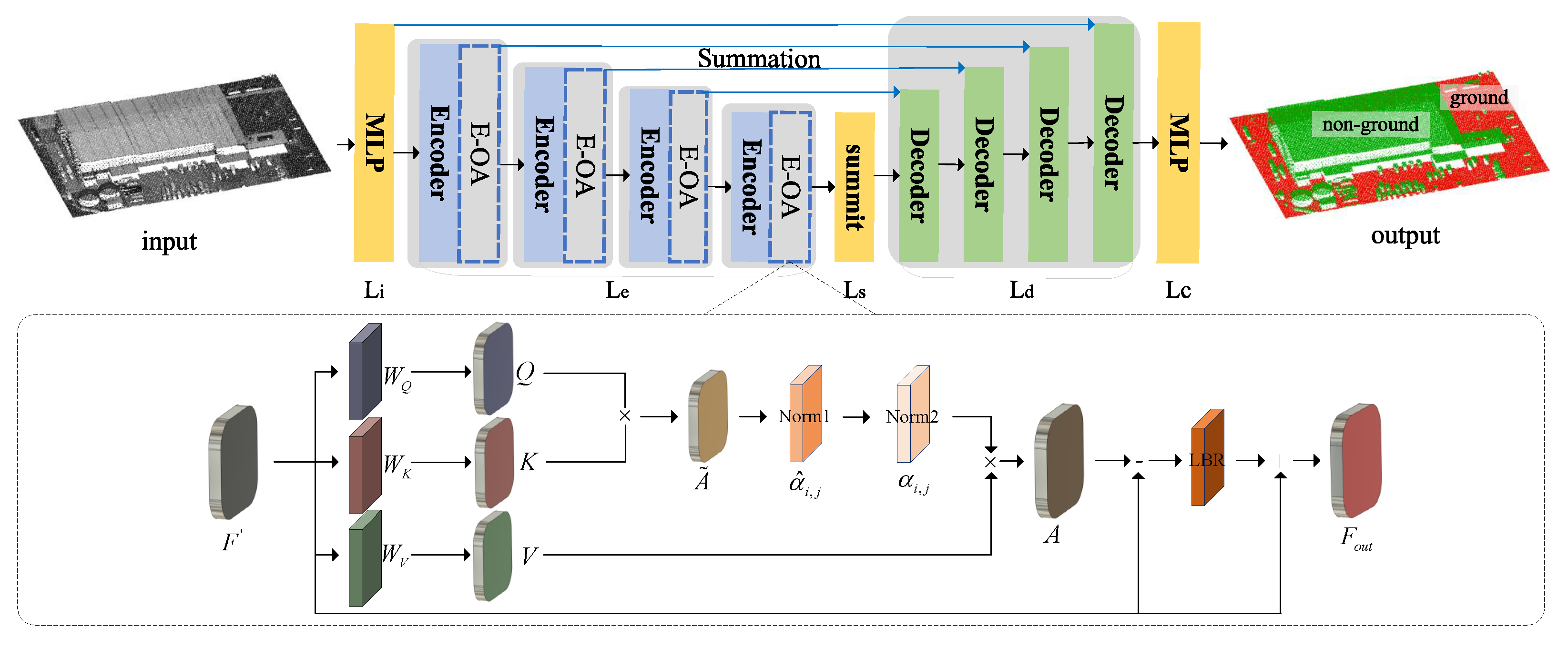
Deep learning frameworks for point clouds encompass five core components as illustrated in Figure 2: input embedding ($L_i$), an encoding layer ($L_e$), a middle layer ($L_s$), a decoding layer ($L_d$), and a classification layer ($L_c$). The type, quantity, and presence of each component can be variably adjusted. Within the input embedding ($L_i$), the features of the input points, denoted as $F\in {\mathbb{R}}^{N\times C}$, are mapped to a high-dimensional space [45]. In the encoding layer ($L_e$), neighborhood searches are performed to identify the K neighbors $\left\{P_i^1,P_i^2,P_i^3,\cdots ,P_i^K\right\}$ for each sampled point $P_i$. The positional relationship between $P_i$ and its neighbors $\left\{P_i^1,P_i^2,P_i^3,\cdots ,P_i^K\right\}$ establishes implicit edges between them [33]. The neighborhood aggregation function $\varphi$ aggregates the neighbor features $F_i=\left\{F_i^1,F_i^2,F_i^3,\cdots ,F_i^K\right\}$ onto the sampled points, represented as $\widehat{F}$. The encoding layer ($L_e$) is constructed by stacking multiple $\varphi$ layers and downsampling layers $\phi$ to reduce the number of points in the point cloud while mapping the features to a higher-dimensional space. The middle layer ($L_s$) is designed to enhance the model’s learning capacity. The decoding layer ($L_d$) upsamples the number of points using the KNN interpolation algorithm [32] and decodes the features. Lastly, the classification layer ($L_c$) decodes the features into a probability distribution representing the number of categories within the point cloud,

$$\mathcal{I}=\phi \left({\varphi }_{k/r}\left(F\in {\mathbb{R}}^{N\times C}\right)\right),$$

(1)

where $\mathcal{I}$ represents the encoding result obtained after stacking a single aggregation layer $\varphi$ and a downsampling layer $\phi$. The final encoding outcome is computed by stacking several layers of $\mathcal{I}$ during the encoding phase. N and C are point clouds and features, respectively.

3.2. Elevation Offset-Attention

Self-Attention Mechanism. The success of attention mechanisms in both the NLP [31,47,48] and image domains [49,50,51] is attributed to their capability to model long-range dependencies. In the context of point cloud data, the attention mechanism has been recognized as an effective method to capture the correlations within unordered point cloud sequences [45]. According to [31], given input features F, we first compute Query, Key, and Value matrices, $Q={\left\{q_i\right\}}_{i=1}^{i=S}$, $K={\left\{k_i\right\}}_{i=1}^{i=S}$, $V={\left\{v_i\right\}}_{i=1}^{i=S}$, as

$$\begin{array}{cc}\hfill & Q=W_Q·F,\hfill \\ \hfill & K=W_K·F,\hfill \\ \hfill & V=W_V·F,\hfill \end{array}$$

(2)

where $W_Q$, $W_K$, $W_V$ are three learnable weight matrices. The self-attention mechanism can be described as

$$\begin{array}{cc}\hfill F_{sa}& ={\left(\alpha \right)}_{i,j}·V\hfill \\ \hfill & =A·V\hfill \\ \hfill & =\delta \tilde{A}·V\hfill \\ \hfill & =\delta (Q·K^T)·V,\hfill \end{array}$$

(3)

where the output from self-attention is denoted as $F_{sa}$. The adjacency weight matrix, $\tilde{A}$, is obtained by calculating the dot product of matrices Q and $K^{\mathrm{T}}$. $\delta$ is employed to normalize $\tilde{A}$. Within $\delta$, $\tilde{A}$ is scaled using ${}^1/\sqrt{d_k}$, where $\sqrt{d_k}$ is determined by the feature dimensions of K. Next, the Softmax is computed, resulting in A as the normalized weight. ${\left(\alpha \right)}_{i,j}$ represents an alternative form of A, indicating the similarity level between the i-th Q and the j-th row of K. By applying A to V, the attention outcome is produced.

The features of $F_{sa}$ are remapped by LBR and the resultant features are added to the input features F, facilitating the direct use of self-attention. The output is denoted as $F_{out}$. LBR refers to the linear, normalization, and activation operations, respectively, as follows:

$$F_{out}=LBR\left(F_{sa}\right)+F.$$

(4)

Elevation Offset-Attention. Differing from Equation (4), the subtraction operation between the input features F and $F_{sa}$ is computed, with the resulting values replacing the original position of $F_{sa}$, denoted as ${\overline{F}}_{sa}$. Consequently, the overall E-OA framework can be described by the following Equation (5):

$$\begin{array}{cc}\hfill F_{out}& =LBR\left({\overline{F}}_{sa}\right)+F\hfill \\ \hfill & =LBR(F-F_{sa})+F.\hfill \end{array}$$

(5)

The normalization operation $\delta$ was modified. As indicated by Equations (1)–(3), the form of the adjacency weight matrix $\tilde{A}$ is $(\ast ,N,N)$. Firstly, Softmax was applied to the column vectors of the $N\times N$ matrix. Following this, the $L_1$ normalization operation was applied to the row vectors of the $N\times N$ matrix, consistent with the procedure in self-attention, as shown in Figure 2. The dual normalization is illustrated as follows:

$$\begin{array}{c}\hfill {\left(\tilde{\alpha }\right)}_{i,j}=Q·K_k^T\end{array}$$

(6)

$$\begin{array}{c}\hfill {\displaystyle {\widehat{\alpha }}_{i,j}=exp\left({\widehat{\alpha }}_{i,j}\right)/\sum _{k}exp\left({\widehat{\alpha }}_{k,j}\right)}\end{array}$$

(7)

$$\begin{array}{c}\hfill {\displaystyle {\alpha }_{i,j}={\widehat{\alpha }}_{i,j}/\sum _k{\widehat{\alpha }}_{i,k}}\end{array}$$

(8)

Regarding the interpretation of F in Equation (5), F encompasses basic spatial coordinates (p) and other attribute features f. In this study, the elevation e is utilized as an independent feature. The feature utilization is detailed as follows:

$$\begin{array}{cc}\hfill F_{out}& =LBR\left(F(p,e,f)\right)-F_{sa})+F(p,e,f),\hfill \end{array}$$

(9)

3.3. Computational Complexity

A schematic representation of the E-OA module’s operation is depicted in Figure 3. It accepts the output features $F^{\prime }$ from each encoding layer $\mathcal{I}$ and establishes relationships for each $F^{\prime }$. Given an input point count of N for $\mathcal{I}$ and a scale factor of S, the corresponding point count for $F^{\prime }$ is $M=N/S$.

Assuming the E-OA module is applied to the input set of N points, the computational complexity is $\mathcal{O}\left(N^2\right)$. This is undoubtedly prohibitive for data batches containing tens of thousands of point clouds. The computational complexity of attention after the first $\mathcal{I}$ layer is $\mathcal{O}\left(M^2\right)$, while for the n-th $\mathcal{I}$ layer, it is $\mathcal{O}\left({(M/(nS\left)\right)}^2\right)$. When directly computed, the complexity is $\mathcal{O}\left(N^2\right)\times n$. Given the high complexity of computing inter-point attention and the significance of the encoder in a model, the E-OA module is employed after $\mathcal{I}$.

3.4. Training Method

In order to compare the impact of E-OA on the performance of different point cloud deep learning frameworks, it is essential to standardize all performance-influencing strategies other than the model framework.

Unified Data Downsampling Strategy. The original data are downsampled using a grid-based downsampling method; during the model training process, the farthest point sampling method is employed for downsampling.

Unified Data Augmentation Strategy. To enhance the effectiveness of the data used [52], we adopted four typical data augmentation methods: (1) Centering. (2) Random rotation around the X-axis or Z-axis within a specified range. This simulates the different observation effects caused by different observation angles. (3) Random scaling, which simulates the different observation effects caused by different distances from the point cloud. (4) Random displacement and drop, which simulates the situation of sensor damage.

4. Results

In this section, the experimental data, evaluation metrics, and experimental results are primarily introduced.

4.1. Train Dataset

To validate the effectiveness of the proposed method, experiments were conducted on two datasets: OpenGF and Navarre. In addition to the coordinates and elevation information, both datasets individually contain intensity and RGB information as input features.

The OpenGF dataset spans four distinct regions situated in four different countries, covering an aggregate area of 47.7 km${}^2$ and encompassing 542.1 MB of point cloud data. It offers a diverse range of terrain scenes, namely urban, suburban, rural, and mountainous. The urban scene is characterized by densely packed large buildings; the suburban terrain presents a mix of undulating and rugged landscapes; rural settings feature sparsely scattered buildings; and the mountainous region is marked by steep slopes and prevalent dense vegetation. The OpenGF data have been meticulously segmented into ground and non-ground classes and were partitioned into tiles measuring 500 × 500 km${}^2$ each. Comprehensive details can be found in [53].

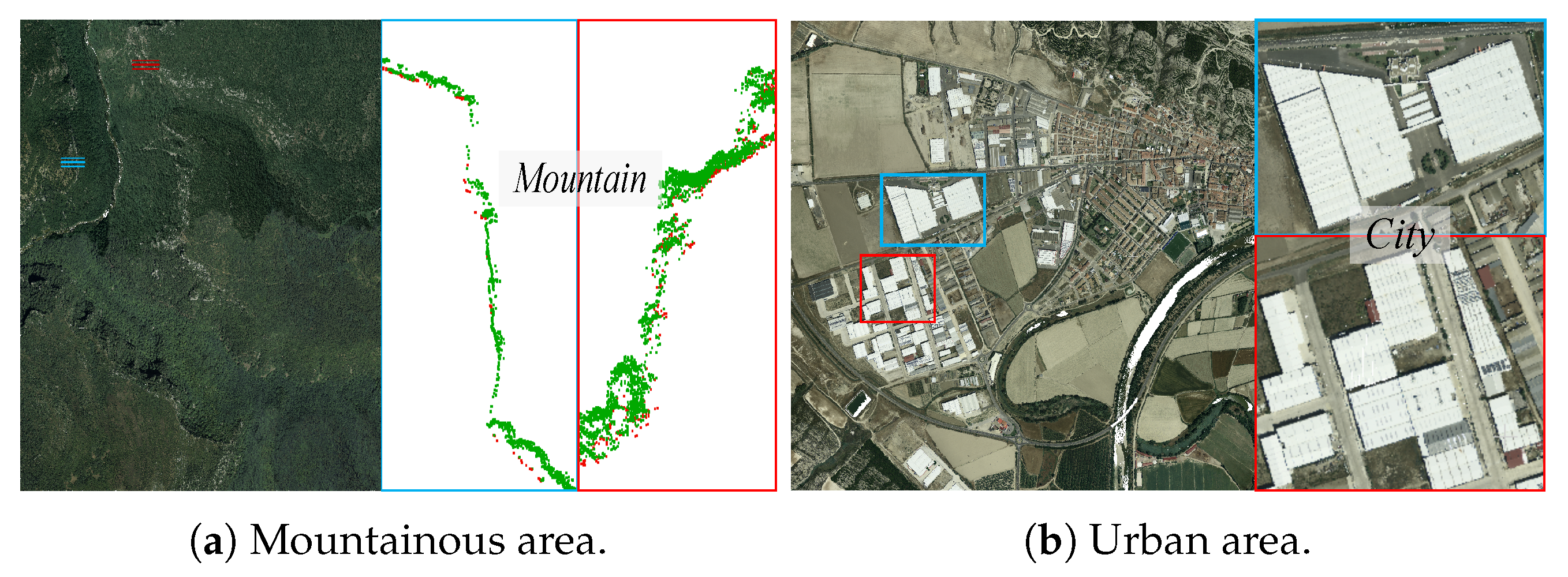
The Navarre dataset, sourced from the Government of Navarra https://cartotecayfototeca.navarra.es/ (accessed on 15 October 2022), utilizes data obtained from the ALS60 linear scan sensors dated between 2011 and 2012 for experimental evaluation. With a point density of 1 point/m${}^2$, the data have been semi-automatically classified and further divided into tiles of 2 × 2 km${}^2$ each. For the study, two distinctive scenes were chosen, leveraging satellite imagery as a reference: (1) urban settings, encompassing buildings of varying dimensions along with expansive factories, and (2) mountainous terrain, characterized by features like mountains, cliffs, valleys, and woodlands. The labels have been restructured, deriving from the official classification, to distinguish between ground and non-ground segments. In total, the curated dataset comprises 71 individual tiles.

4.2. Test Dataset

The OpenGF and Navarre datasets each contain two test sets. Within the OpenGF dataset, Test I encompasses three distinct terrains: a village, a mountainous region, and a smaller urban setting. Test II presents an urban landscape, notably featuring a structure that exceeds 200 m in both length and width. A detailed description of this can be found in [53] and will not be elaborated further here. For the Navarre dataset, two test sets were meticulously designed. Test I captures features such as high-altitude cliffs, profound gorges, and pronounced inclines, as illustrated in Figure 4a. Conversely, Test II showcases an urban environment dominated by a building measuring 265 m in length and 70 m in width, as depicted in Figure 4b. The presence of large-scale structures and canyons poses significant challenges to the performance of the model. A comprehensive breakdown of these test sets is provided in

Table 1. Test set parameters.

Dataset	Coverage	Density (Points/m${}^2$)	Non-Ground (Points)	Ground (Points)
OpenGF Test I	6.6 km${}^2$	6	10,431,224	5,332,664
OpenGF Test II	1.1 km${}^2$	14	962,357	752,242
Navarre Test I	2 km${}^2$	1	7,137,467	976,293
Navarre Test II	2 km${}^2$	1	1,267,144	2,331,908

.

4.3. Experimental Parameters and Evaluation Indicators

Experiments were executed on a consistent server configuration, featuring an Intel(R) Xeon(R) CPU E5-2680 v4 @ 2.40 GHz, 251 GB of RAM, and an NVIDIA RTX 3090 GPU.

Training Parameters. Uniform training parameters were employed across all models. The initial learning rate was fixed at 0.01, and a cosine annealing approach was adopted for learning rate adjustments. The network was trained for 500 epochs using the AdamW optimizer, with a consistent batch size of 4 and each batch comprising $4\times {10}^4$ points.

Evaluation Metrics. In this study, metric evaluations were derived from the union and intersection ratios across all categories, as well as for individual categories. These ratios were denoted as $mIOU$ for overall recognition accuracy, $IO{U}_1$ for non-ground recognition accuracy, and $IO{U}_2$ for ground recognition accuracy. The accuracy was also used to denote the overall recognition accuracy.

$$\begin{array}{cc}\hfill IO{U}_1& =\frac{TP}{(TP+FN+FP)}\hfill \\ \hfill IO{U}_2& =\frac{TN}{(FN+FP+TN)}\hfill \\ \hfill mIOU& =\frac{IO{U}_1+IO{U}_2}{2}\hfill \\ \hfill Accuracy& =\frac{(TP+TN)}{(TP+FN+FP+TN)}\hfill \end{array}$$

(10)

where the variables $TP$, $FN$, $FP$, and $TN$ denote the number of correctly classified non-ground points, the number of ground points erroneously classified as non-ground, the number of non-ground points incorrectly classified as ground, and the number of correctly classified ground points, respectively.

4.4. Validation Analysis on OpenGF Test Set

Experiments were conducted using two traditional methods, PMF [54] and CSF [55]; three conventional point cloud deep learning methods, RandLA-Net [34], point transformer [42], and PointMeta-L [56]; and one pure transformer model, CDFormer [57].

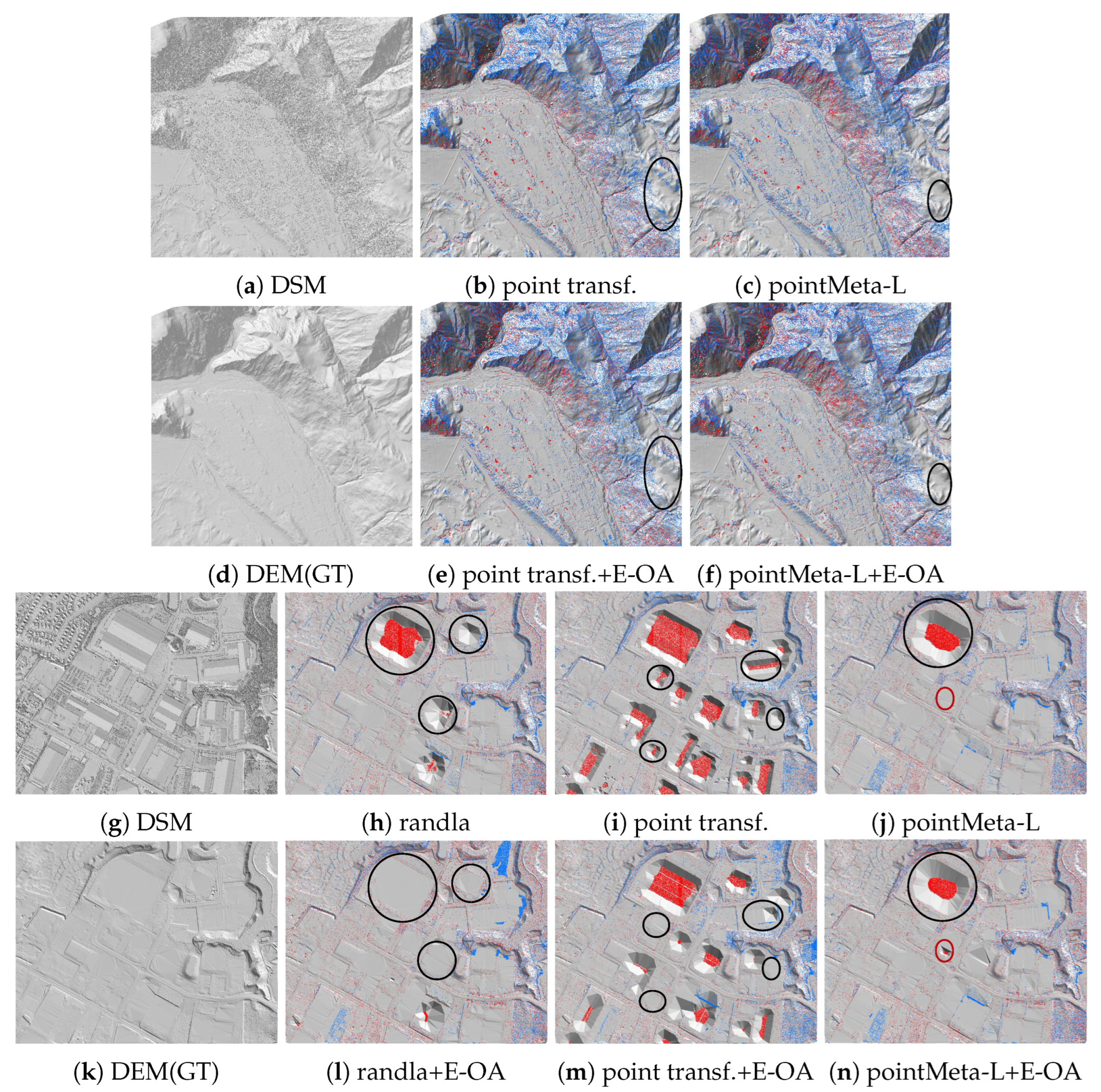
The experiment focused on the ground filtering performance of models, particularly on $IO{U}_2$. The results are displayed in

Table 2. The quantitative evaluation results on the OpenGF test set.

Method	Test I				Test II
	$\mathit{Ac}$	$\mathit{mIOU}$	${\mathit{IoU}}_{\mathbf{1}}$	${\mathit{IoU}}_{\mathbf{2}}$	$\mathit{Ac}$	$\mathit{mIOU}$	${\mathit{IoU}}_{\mathbf{1}}$	${\mathit{IoU}}_{\mathbf{2}}$
PMF	0.9063	0.8242	0.8522	0.7962	0.8656	0.7606	0.7850	0.7361
CSF	0.9306	0.8691	0.8817	0.8564	0.8934	0.8073	0.8108	0.8038
RandLA-Net	0.9766	0.9487	0.9657	0.9318	0.9533	0.9101	0.918	0.9022
RandLA-Net+E-OA	0.9761	0.9485	0.9650	0.9319	0.9596	0.9213	0.9301	0.9126
Point transformer	0.9743	0.9436	0.9625	0.9247	0.9144	0.8468	0.8503	0.8433
Point transformer+E-OA	0.9770	0.9495	0.9662	0.9328	0.9392	0.8845	0.8951	0.8738
PointMeta-L	0.9661	0.9259	0.9510	0.9008	0.9486	0.9010	0.9116	0.8903
PointMeta-L+E-OA	0.9748	0.9448	0.9631	0.9266	0.9578	0.9182	0.9262	0.9102
CDFormer	0.9717	0.9382	0.9586	0.9179	0.9421	0.8897	0.8988	0.8806

. Both traditional methods exhibited a poor ground classification accuracy, indicating inadequate ground filtering results (the results are from [53]). As per Section 3, we integrated the E-OA module into three conventional point cloud frameworks, leading to an overall enhancement in the model performance. In Test I, which covers mountainous areas, the enhanced point transformer demonstrated the best filtering effect, with an $IO{U}_2$ increase of 0.81% compared to the baseline model. The most significant improvement was observed for PointMeta-L, with an increase of 2.58% in the $IO{U}_2$ value; however, improvements in RandLA-Net were not substantial. The corresponding results are depicted in Figure 5b,c,e,f). Due to the only marginal improvement in RandLA-Net, it is not distinctly visible in the figure and is therefore not listed here. In Test II, the enhanced versions of all three conventional point cloud frameworks showed performance improvements, with increases of 1.04%, 3.05%, and 1.83%, respectively. Among these, the RandLA-Net model with the E-OA module excelled in filtering large buildings, as shown in Figure 5h,l. The improved versions of point transformer and PointMeta-L showed slight increases in $IO{U}_2$ values, but a lower filtering effectiveness, possibly due to their framework designs, as seen in Figure 5i,j,m,n). Notably, the filtering ability of RandLA-Net in urban areas with large buildings was discussed in [53], and our experimental outcomes reaffirmed this. CDFormer, an attention-based framework, underperformed compared to the improved baseline models in mountainous regions and was less effective than the enhanced RandLA-Net and PointMeta-L in urban settings. This underscores the necessity of the aim of our experiments: how to better utilize attention mechanisms.

4.5. Validation Analysis on the Navarre Test Set

Table 3. The quantitative evaluation results on the Navarre test set.

Method	Test I				Test II
	$\mathit{Ac}$	$\mathit{mIOU}$	${\mathit{IoU}}_{\mathbf{1}}$	${\mathit{IoU}}_{\mathbf{2}}$	$\mathit{Ac}$	$\mathit{mIOU}$	${\mathit{IoU}}_{\mathbf{1}}$	${\mathit{IoU}}_{\mathbf{2}}$
PMF	0.8512	0.6290	0.8328	0.4253	0.8543	0.6414	0.4729	0.8100
CSF	0.8105	0.5278	0.7970	0.2585	0.8186	0.6549	0.5403	0.7695
RandLA-Net	0.9461	0.7836	0.9408	0.6264	0.9443	0.8899	0.8675	0.9124
RandLA-Net+E-OA	0.9519	0.8170	0.9462	0.6879	0.9504	0.9012	0.8804	0.9220
Point transformer	0.9487	0.8106	0.9425	0.6786	0.951	0.9023	0.8818	0.9227
Point transformer+E-OA	0.9509	0.8147	0.9450	0.6844	0.9489	0.8985	0.8779	0.9191
PointMeta-L	0.9386	0.7765	0.9314	0.6216	0.9293	0.8623	0.8343	0.8903
PointMeta-L+E-OA	0.9408	0.7852	0.9339	0.6365	0.9374	0.8758	0.8487	0.9028
CDFormer	0.9288	0.7518	0.9210	0.5825	0.8903	0.7740	0.6939	0.8540

provides the quantitative assessment results on the Navarre test dataset. The parameters of the two traditional methods were fine-tuned to their optimum settings, yet yielded the poorest filtering performance. In the mountainous region (Test I), the improved versions of the three baseline models exhibited increases in their $IO{U}_2$ values by 6.15%, 0.58%, and 0.91%, respectively. In urban areas (Test II), the enhancements in $IO{U}_2$ values for the improved versions of RandLA-Net and PointMeta-L were 0.96% and 1.25%, respectively, while the enhanced point transformer showed no improvement, mirroring its performance on the OpenGF dataset. Due to the minimal improvement in the point transformer in Test I and its unsatisfactory performance on Test II, only the classification results of RandLA-Net and PointMeta are shown in Figure 6, with areas of significant changes highlighted using black circles or rectangles. It is important to note that due to erroneous annotations in overlapping areas of the Navarre dataset, there are stripe artifacts in the classification results in Figure 6g–l, but these do not affect the comparison of all models’ performances. The advanced CDFormer framework did not exhibit a ground filtering performance comparable to point cloud frameworks equipped with the E-OA attention mechanism in both mountainous and urban areas.

5. Discussion

This section presents ablation studies conducted to evaluate the proposed method. The impact of grid sampling size and global scene size on experimental results is discussed; additionally, comparisons are made with three current global modeling frameworks. Furthermore, the effective receptive field is visualized to fully substantiate the reliability of the method proposed in this paper.

5.1. Impact of Different Grid Subsampling Sizes

To assess the impact of varying grid sampling sizes on point cloud classification outcomes, the RandLA-Net network was selected for comparative experiments on the OpenGF Test II dataset. As verified in Section 4.4, the RandLA-Net network demonstrates a robust classification performance for large buildings. OpenGF Test II, which includes a significant building structure, aptly illustrates the results of these comparative experiments. Four distinct grid sampling sizes were employed, 0.25 m, 0.5 m, 0.75 m, and 1 m, with the experimental outcomes presented in

Table 4. Impact of sampling rate results.

Downsampling (m)	$\mathit{Ac}$	$\mathit{mIOU}$	${\mathit{IoU}}_1$	${\mathit{IoU}}_2$
0.25	0.9281	0.8659	0.8639	0.8678
0.5	0.9415	0.8895	0.8926	0.8863
0.75	0.9522	0.9082	0.9154	0.9010
1.0	0.9596	0.9213	0.9301	0.9126

and Figure 7. It was observed that different grid sampling sizes exert varied impacts on building classification. Specifically, a decrease in grid size led to a reduction in classification accuracy. Notably, the RandLA-Net model, when equipped with global semantic information, consistently maintained effective results in filtering large buildings on the ground at a grid sampling size of 0.5 m. In other words, integrating local and global information within the RandLA-Net model ensures commendable performance, provided the grid size exceeds 0.5 m. Furthermore, we recommend a maximum sampling grid of 1 m, as larger sampling grids would result in the loss of local terrain information.

5.2. Impact of Global Scene Size

When analyzing the impact of the number of points in each global scene on the model’s classification results, it is recognized that loading all point clouds from a tile into the model at once is impractical. In deep learning, batch loading for inference is a feasible method, yet the number of point clouds in a single batch can affect the model’s classification results. Hence, we compared and analyzed cases with point cloud numbers in a single batch at $5\times {10}^3$, $1\times {10}^4$, and $2\times {10}^4$, as illustrated in Figure 8. Experiments were conducted using an improved version of RandLA-Net, with the results presented in

Table 5. Impact of scene size on filtering performance.

Points	$\mathit{Ac}$	$\mathit{mIOU}$	${\mathit{IoU}}_1$	${\mathit{IoU}}_2$
$2\times {10}^4$	0.9610	0.9240	0.9324	0.9156
$1\times {10}^4$	0.9572	0.9170	0.9254	0.9087
$5\times {10}^3$	0.9502	0.9043	0.9128	0.8958

. When the number of points is low, such as $5\times {10}^3$, the model’s classification accuracy is insufficient. With an increase in the point cloud number to $1\times {10}^4$, the classification results still show inadequacies. However, when the point cloud number further rises to $2\times {10}^4$, it is observed that most ground buildings, especially buildings, are effectively filtered out. This analysis indicates that more scene information provides additional background context, aiding the E-OA module in driving the network to learn more semantic information, thereby enhancing the network’s filtering capability.

5.3. Comparison of Different Attention Mechanisms

To further substantiate the superiority of the E-OA module in handling large-scale point cloud data, several state-of-the-art attention mechanisms were compared. External attention [58] utilizes a compact token set (S) as an external memory unit to interact with the input for deriving attention weights, with a computational complexity of $\mathcal{O}\left(SN\right)$. In this study, S was set to 512. APPT [46] is a framework that utilizes proxy points to reduce computational complexity. It initially aggregates information from each group of neighbors to the sampled center, i.e., the proxy point, and subsequently calculates attention weights between the proxy point and all original points, resulting in a complexity of $\mathcal{O}\left(MN\right)$, where M is determined by the downsampling rate. CDFormer [57], another framework seeking to lower computational complexity via proxy points, initially computes attention weights within each set of neighbors and consolidates neighbor information onto proxy points, with a complexity of $\mathcal{O}\left(M{k}^2\right)$. Subsequently, it computes the weights for each group of proxy points with a complexity of $\mathcal{O}\left(M{k}^2\right)$, and finally distributes the proxy point information back to the initial input points with a complexity of $\mathcal{O}\left(N{k}^2\right)$. In comparison, the computational complexity of the E-OA module is less than that of APPT, but greater than the others.

Table 6. Comparison of attention performance.

Method	Test I				Test II
	$\mathit{Ac}$	$\mathit{mIOU}$	${\mathit{IoU}}_{\mathbf{1}}$	${\mathit{IoU}}_{\mathbf{2}}$	$\mathit{Ac}$	$\mathit{mIOU}$	${\mathit{IoU}}_{\mathbf{1}}$	${\mathit{IoU}}_{\mathbf{2}}$
RandLA-Net + External	0.9701	0.9431	0.9582	0.9280	0.9563	0.9169	0.9230	0.9108
RandLA-Net + APPT	0.9696	0.9419	0.9596	0.9242	0.9513	0.9144	0.9233	0.9055
RandLA-Net + CDFormer	0.9534	0.8993	0.9337	0.8648	0.8945	0.8086	0.8192	0.7979
RandLA-Net + E-OA	0.9761	0.9485	0.9650	0.9319	0.9596	0.9213	0.9301	0.9126

below presents the results of embedding the aforementioned attention mechanisms into the RandLA-Net model at the same position as the E-OA module and conducting experiments on OpenGF’s test I and II. The experimental results demonstrate that the E-OA module exhibits clear advantages in processing large spatial point clouds.

5.4. Effective Receptive Field Analysis

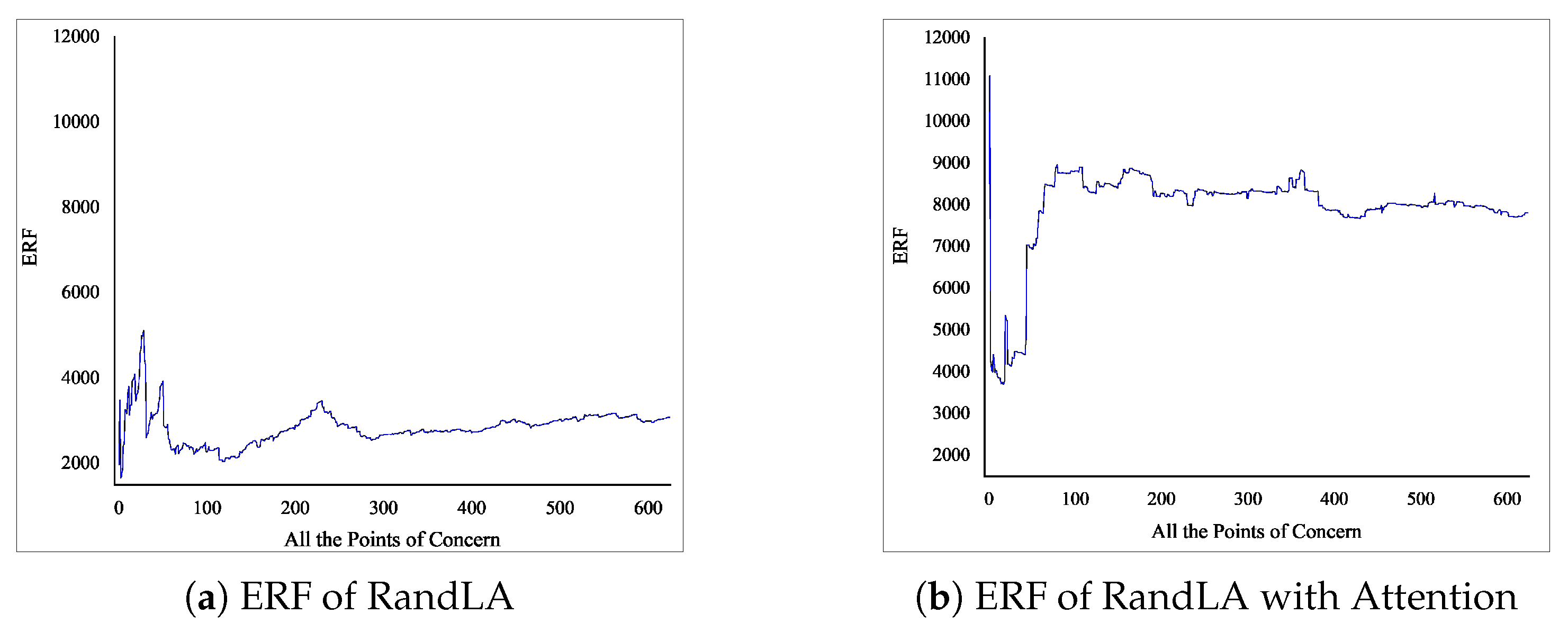
The Effective Receptive Field (ERF) represents the distribution of high-density point clouds contributing to the network model, serving as an efficient means to evaluate the performance of the global module. In this paper, we conduct experiments on OpenGF test I and qualitatively compare the baseline and improved versions of the RandLA-Net, as illustrated in Figure 9 and Figure 10. The baseline RandLA-Net primarily focuses on the local areas of the point cloud, whereas the improved version captures a considerable amount of useful information. To further substantiate the efficacy of our proposed method, we present statistical values of the ERFs for 625 points of interest in Figure 10. We analyze the ERFs of all points in the first decoding layer, as the weights of this layer have been propagated through the transformer layer and encompass an appropriate quantity of point clouds. We quantified the number of ERFs considered effective and discovered that models with global capabilities achieve higher attention coverage on the rooftops of buildings, which further validates the effectiveness of our approach.

6. Conclusions

In this paper, we address the challenges of modeling geographical relationships based on large-scale airborne LiDAR point cloud data. We critically analyzed the limitations of existing traditional and deep-learning-based terrain filtering methods from point clouds, highlighting the significance of constructing remote relationships in airborne point cloud terrain filtering and integrating global and local modeling for experimental analysis. A novel global semantic capture module, E-OA, is introduced, designed to enhance model performance by combining it with existing networks that capture local information. For a fair comparison, we restructured three classic point cloud deep neural networks, standardized training strategies, and incorporated the E-OA module into these frameworks for comparative experiments. These experiments were conducted on two datasets, each characterized by different data features.

Given that each point in a point cloud can be considered as an individual semantic unit, directly inputting tens of thousands of points into the model for global relationship construction proved to be impractical. Hence, we analyzed computational complexities and decided to integrate the E-OA module into the encoding layers of the base frameworks, placing it after each downsampling layer. This approach not only reduced the computational complexity but also ensured that the points involved in the computation carried local information. The experimental results demonstrated that the E-OA module enhanced the performance of the benchmark models to varying degrees across different data sources. For urban areas, the RandLA-Net equipped with the E-OA module excelled, while the point transformer with the E-OA module was superior in mountainous regions. By introducing the E-OA module into the benchmark models, the models were encouraged to move beyond their local “comfort zones”.

In future work, we aim to continue exploring the design principles of different frameworks to elucidate how various forms of global attention impact the network’s terrain filtering performance. Additionally, we plan to further investigate compact global modeling frameworks for integration into airborne devices, enhancing their efficiency and applicability in terrain filtering tasks.

References

1. Du, L.; McCarty, G.W.; Zhang, X.; Lang, M.W.; Vanderhoof, M.K.; Li, X.; Huang, C.; Lee, S.; Zou, Z. Mapping Forested Wetland Inundation in the Delmarva Peninsula, USA Using Deep Convolutional Neural Networks. Remote Sens. 2020, 12, 644. [Google Scholar] [CrossRef]
2. Li, D.; Tang, X.; Tu, Z.; Fang, C.; Ju, Y. Automatic Detection of Forested Landslides: A Case Study in Jiuzhaigou County, China. Remote Sens. 2023, 15, 3850. [Google Scholar] [CrossRef]
3. Chen, Z.; Ye, F.; Fu, W. The influence of DEM spatial resolution on landslide susceptibility mapping in the Baxie River basin, NW China. Nat. Hazards 2020, 101, 853–877. [Google Scholar] [CrossRef]
4. Kakavas, M.P.; Nikolakopoulos, K.G. Digital Elevation Models of Rockfalls and Landslides: A Review and Meta-Analysis. Geosciences 2021, 11, 256. [Google Scholar] [CrossRef]
5. McClean, F.; Dawson, R.; Kilsby, C. Implications of Using Global Digital Elevation Models for Flood Risk Analysis in Cities. Water Resour. Res. 2020, 56, e2020WR028241. [Google Scholar] [CrossRef]
6. Ozendi, M.; Akca, D. A point cloud filtering method based on anisotropic error model. Photogramm. Rec. 2023, 38, 1–38. [Google Scholar] [CrossRef]
7. Gökgöz, T.; Baker, M.K.M. Large Scale Landform Mapping Using Lidar DEM. ISPRS Int. J. Geo-Inf. 2015, 4, 1336–1345. [Google Scholar] [CrossRef]
8. O’Banion, M.S.; Olsen, M.J.; Hollenbeck, J.P.; Wright, W.C. Data Gap Classification for Terrestrial Laser Scanning-Derived Digital Elevation Models. ISPRS Int. J. Geo-Inf. 2020, 9, 749. [Google Scholar] [CrossRef]
9. Buján, S.; González-Ferreiro, E.M.; Cordero, M.; Miranda, D. PpC: A new method to reduce the density of lidar data. Does it affect the DEM accuracy? Photogramm. Rec. 2019, 34, 304–329. [Google Scholar] [CrossRef]
10. Susaki, J. Adaptive Slope Filtering of Airborne LiDAR Data in Urban Areas for Digital Terrain Model (DTM) Generation. Remote Sens. 2012, 4, 1804–1819. [Google Scholar] [CrossRef]
11. Evans, J.S.; Hudak, A.T. A Multiscale Curvature Algorithm for Classifying Discrete Return LiDAR in Forested Environments. IEEE T. Geosci. Remote 2007, 45, 1029–1038. [Google Scholar] [CrossRef]
12. Yan, W.Y. Scan Line Void Filling of Airborne LiDAR Point Clouds for Hydroflattening DEM. IEEE J.-STARS 2021, 14, 6426–6437. [Google Scholar] [CrossRef]
13. Pan, Z.; Tang, J.; Tjahjadi, T.; Wu, Z.; Xiao, X. A Novel Rapid Method for Viewshed Computation on DEM through Max-Pooling and Min-Expected Height. ISPRS Int. J. Geo-Inf. 2020, 9, 633. [Google Scholar] [CrossRef]
14. Medeiros, S.C.; Bobinsky, J.S.; Abdelwahab, K. Locality of Topographic Ground Truth Data for Salt Marsh Lidar DEM Elevation Bias Mitigation. IEEE J-STARS 2022, 15, 5766–5775. [Google Scholar] [CrossRef]
15. Cao, S.; Pan, S.; Guan, H. Random forest-based land-use classification using multispectral LiDAR data. Bull. Surv. Mapp. 2019, 11, 79–84. [Google Scholar] [CrossRef]
16. Wu, J.; Liu, L. Automatic DEM generation from aerial lidar data using multiscale support vector machines. Mippr 2011 Remote Sens. Image Process. Geogr. Inf. Syst. Other Appl. 2011, 8006, 63–69. [Google Scholar] [CrossRef]
17. Lodha, S.; Kreps, E.; Helmbold, D.; Fitzpatrick, D. Aerial LiDAR data classification using support vector machines (SVM). In Proceedings of the Third International Symposium on 3D Data Processing, Visualization, and Transmission, Chapel Hill, NC, USA, 14–16 June 2006; pp. 567–574. [Google Scholar] [CrossRef]
18. Wu, J.; Guo, N.; Liu, R.; Xu, G. Aerial Lidar Data Classification Using Weighted Support Vector Machines. Int. Conf. Digit. Image Process. 2013, 38, 1–5. [Google Scholar]
19. Niemeyer, J.; Wegner, J.D.; Mallet, C.; Rottensteiner, F.; Soergel, U. Conditional Random Fields for Urban Scene Classification with Full Waveform LiDAR Data. Photogramm. Image Anal. ISPRS Conf. 2011, 6952, 233–244. [Google Scholar] [CrossRef]
20. Zheng, Y.; Cao, Z.G. Classification method for aerial LiDAR data based on Markov random field. Electron. Lett. 2011, 47, 934. [Google Scholar] [CrossRef]
21. Luo, W.; Ma, H.; Yuan, J.; Zhang, L.; Ma, H.; Cai, Z.; Zhou, W. High-Accuracy Filtering of Forest Scenes Based on Full-Waveform LiDAR Data and Hyperspectral Images. Remote Sens. 2023, 15, 3499. [Google Scholar] [CrossRef]
22. Charles, R.Q.; Su, H.; Kaichun, M.; Guibas, L.J. PointNet: Deep Learning on Point Sets for 3D Classification and Segmentation. In Proceedings of the IEEE Conference on Computer Vision and Pattern Recognition (CVPR), Honolulu, HI, USA, 21–26 July 2017; pp. 77–85. [Google Scholar] [CrossRef]
23. Li, Y.; Bu, R.; Sun, M.; Wu, W.; Di, X.; Chen, B. PointCNN: Convolution on x-transformed points. In Proceedings of the Advances in Neural Information Processing Systems, Montreal, QC, Canada, 2–8 December 2018; pp. 820–830. [Google Scholar] [CrossRef]
24. Kim, Y. Convolutional Neural Networks for Sentence Classification. In Proceedings of the 2014 Conference on Empirical Methods in Natural Language Processing (EMNLP), Doha, Qatar, 25–29 October 2014; Association for Computational Linguistics: Doha, Qatar, 2014; pp. 1746–1751. [Google Scholar] [CrossRef]
25. Liu, Z.; Sun, M.; Zhou, T.; Huang, G.; Darrell, T. Rethinking the value of network pruning. In Proceedings of the Seventh International Conference on Learning Representations (ICLR), New Orleans, LA, USA, 6–9 May 2019; pp. 2818–2826. [Google Scholar] [CrossRef]
26. Lu, Z.; Xu, C.; Du, B.; Ishida, T.; Zhang, L.; Sugiyama, M. LocalDrop: A Hybrid Regularization for Deep Neural Networks. IEEE T. Pattern Anal. 2021, 44, 3590–3601. [Google Scholar] [CrossRef] [PubMed]
27. Lei, H.; Akhtar, N.; Mian, A. Spherical Convolutional Neural Network for 3D Point Clouds. In Proceedings of the IEEE/CVF Conference on Computer Vision and Pattern Recognition, Long Beach, CA, USA, 15–20 June 2019; pp. 9631–9640. [Google Scholar] [CrossRef]
28. Fu, K.; Liu, S.; Luo, X.; Wang, M. Robust Point Cloud Registration Framework Based on Deep Graph Matching. In Proceedings of the IEEE Conference on Computer Vision and Pattern Recognition, CVPR 2021, Virtual, 19–25 June 2021; IEEE: New York, NY, USA, 2021; pp. 8893–8902. [Google Scholar] [CrossRef]
29. Yan, X.; Zheng, C.; Li, Z.; Wang, S.; Cui, S. PointASNL: Robust Point Clouds Processing Using Nonlocal Neural Networks with Adaptive Sampling. In Proceedings of the IEEE/CVF Conference on Computer Vision and Pattern Recognition, Seattle, WA, USA, 13–19 June 2020; pp. 5588–5597. [Google Scholar] [CrossRef]
30. Pan, X.; Xia, Z.; Song, S.; Li, L.E.; Huang, G. 3d object detection with pointformer. In Proceedings of the IEEE/CVF Conference on Computer Vision and Pattern Recognition, Nashville, TN, USA, 20–25 June 2021; pp. 7463–7472. [Google Scholar] [CrossRef]
31. Vaswani, A.; Shazeer, N.; Parmar, N.; Uszkoreit, J.; Jones, L.; Gomez, A.N.; Kaiser, L.; Polosukhin, I. Attention is All You Need. NIPS 2017, 30, 1–15. [Google Scholar] [CrossRef]
32. Qi, C.R.; Yi, L.; Su, H.; Guibas, L.J. PointNet++: Deep hierarchical feature learning on point sets in a metric space. NIPS 2017, 30, 1–14. [Google Scholar] [CrossRef]
33. Wu, B.; Liu, Y.; Lang, B.; Huang, L. DGCNN: Disordered Graph Convolutional Neural Network Based on the Gaussian Mixture Model. Neurocomputing 2017, 321, 346–356. [Google Scholar] [CrossRef]
34. Hu, Q.; Yang, B.; Xie, L.; Rosa, S.; Guo, Y.; Wang, Z.; Trigoni, N.; Markham, A. RandLA-Net: Efficient Semantic Segmentation of Large-Scale Point Clouds. In Proceedings of the IEEE Conference on Computer Vision and Pattern Recognition (CVPR), Seattle, WA, USA, 13–19 June 2020; pp. 11105–11114. [Google Scholar] [CrossRef]
35. Thomas, H.; Qi, C.R.; Deschaud, J.E.; Marcotegui, B.; Goulette, F.; Guibas, L. KPConv: Flexible and Deformable Convolution for Point Clouds. In Proceedings of the 2019 IEEE/CVF International Conference on Computer Vision (ICCV), Seoul, Republic of Korea, 27 October–2 November 2019; pp. 6410–6419. [Google Scholar] [CrossRef]
36. Su, H.; Jampani, V.; Sun, D.; Maji, S.; Kalogerakis, E.; Yang, M.; Kautz, J. SPLATNet: Sparse Lattice Networks for Point Cloud Processing. In Proceedings of the 2018 IEEE Conference on Computer Vision and Pattern Recognition (CVPR 2018), Salt Lake City, UT, USA, 18–22 June 2018; pp. 2530–2539. [Google Scholar] [CrossRef]
37. You, Y.; Lou, Y.; Liu, Q.; Tai, Y.; Ma, L.; Lu, C.; Wang, W. Pointwise Rotation-Invariant Network with Adaptive Sampling and 3D Spherical Voxel Convolution. CVPR 2019, 34, 12717–12724. [Google Scholar] [CrossRef]
38. Shi, S.; Guo, C.; Jiang, L.; Wang, Z.; Shi, J.; Wang, X.; Li, H. PV-RCNN: Point-Voxel Feature Set Abstraction for 3D Object Detection. In Proceedings of the IEEE/CVF International Conference on Computer Vision (ICCV), Seoul, Republic of Korea, 27 October–2 November 2019; pp. 10529–10538. [Google Scholar] [CrossRef]
39. Parmar, N.; Vaswani, A.; Uszkoreit, J.; Kaiser, L.; Shazeer, N.; Ku, A.; Tran, D. Image transformer. In Proceedings of the International Conference on Machine Learning PMLR, Stockholm, Sweden, 10–15 July 2018; pp. 4055–4064. [Google Scholar] [CrossRef]
40. Huang, S.; Chen, Y.; Jia, J.; Wang, L. Multi-View Transformer for 3D Visual Grounding. In Proceedings of the IEEE/CVF Conference on Computer Vision and Pattern Recognition (CVPR), New Orleans, LA, USA, 18–24 June 2022; pp. 15524–15533. [Google Scholar] [CrossRef]
41. Hui, L.; Wang, L.; Tang, L.; Lan, K.; Xie, J.; Yang, J. 3D Siamese Transformer Network for Single Object Tracking on Point Clouds. ECCV 2022, 13662, 293–310. [Google Scholar] [CrossRef]
42. Zhao, H. Point transformer. In Proceedings of the IEEE/CVF International Conference on Computer Vision, Montreal, QC, Canada, 11–17 October 2021; pp. 16259–16268. [Google Scholar] [CrossRef]
43. Lu, D.; Xie, Q.; Xu, L.; Li, J. 3DCTN: 3D Convolution-Transformer Network for Point Cloud Classification. IEEE T. Intell. Transp. 2022, 23, 24854–24865. [Google Scholar] [CrossRef]
44. Gao, Y.; Liu, X.; Li, J.; Fang, Z.; Jiang, X.; Huq, K.M.S. LFT-Net: Local feature transformer network for point clouds analysis. IEEE Trans. Intell. Transp. Syst. 2022, 24, 2158–2168. [Google Scholar] [CrossRef]
45. Guo, M.; Cai, J.; Liu, Z.; Mu, T.; Martin, R.R.; Hu, S. PCT: Point cloud transformer. Comput. Vis. Media 2021, 7, 187–199. [Google Scholar] [CrossRef]
46. Li, H.; Zheng, T.; Chi, Z.; Yang, Z.; Wang, W.; Wu, B.; Lin, B.; Cai, D. APPT: Asymmetric Parallel Point Transformer for 3D Point Cloud Understanding. arXiv 2023, arXiv:2303.17815. [Google Scholar] [CrossRef]
47. Devlin, J.; Chang, M.W.; Lee, K.; Toutanova, K. BERT: Pre-training of Deep Bidirectional Transformers for Language Understanding. In Proceedings of the Conference of the North American Chapter of the Association for Computational Linguistics: Human Language Technologies, Minneapolis, MN, USA, 2–7 June 2019; pp. 4171–4186. [Google Scholar] [CrossRef]
48. Yang, Z.; Dai, Z.; Yang, Y.; Carbonell, J.; Salakhutdinov, R.; Le, V.Q. XLNet: Generalized Autoregressive Pretraining for Language Understanding. arXiv 2019, arXiv:1906.08237. [CrossRef]. [Google Scholar]
49. Fu, J.; Liu, J.; Jiang, J.; Li, Y.; Bao, Y.; Lu, H. Scene segmentation with dual relation-aware attention network. IEEE Trans. Neural Netw. Learn. Syst. 2020, 32, 2547–2560. [Google Scholar] [CrossRef]
50. Hu, J.; Shen, L.; Sun, G. Squeeze-and-Excitation Networks. In Proceedings of the IEEE Conference on Computer Vision and Pattern Recognition, Salt Lake City, UT, USA, 18–22 June 2018; pp. 7132–7141. [Google Scholar] [CrossRef]
51. Wang, X.; Girshick, R.; Gupta, A.; He, K. Non-local neural networks. In Proceedings of the IEEE Conference on Computer Vision and Pattern Recognition (CVPR), Salt Lake City, UT, USA, 18–22 June 2018; pp. 7794–7803. [Google Scholar] [CrossRef]
52. Xiao, C.; Wachs, J.; Xiao, C.; Wachs, J. Triangle-net: Towards robustness in point cloud learning. In Proceedings of the IEEE/CVF Winter Conference on Applications of Computer Vision, Waikoloa, HI, USA, 3–8 January 2021; pp. 826–835. [Google Scholar] [CrossRef]
53. Qin, N.; Tan, W.; Ma, L.; Zhang, D.; Li, J. OpenGF: An Ultra-Large-Scale Ground Filtering Dataset Built upon Open ALS Point Clouds around the World. In Proceedings of the IEEE Computer Society Conference on Computer Vision and Pattern Recognition Workshops, Nashville, TN, USA, 19–25 June 2021. [Google Scholar] [CrossRef]
54. Zhang, K.; Chen, S.; Whitman, D.; Shyu, M.; Yan, J.; Zhang, C. A progressive morphological filter for removing nonground measurements from airborne LIDAR data. IEEE T. Geosci. Remote 2003, 41, 872–882. [Google Scholar] [CrossRef]
55. Zhang, W.; Qi, J.; Wan, P.; Wang, H.; Xie, D.; Wang, X.; Yan, G. An Easy-to-Use Airborne LiDAR Data Filtering Method Based on Cloth Simulation. Remote Sens. 2016, 8, 501. [Google Scholar] [CrossRef]
56. Lin, H.; Zheng, X.; Li, L.; Chao, F.; Wang, S.; Wang, Y.; Tian, Y.; Ji, R. Meta Architecure for Point Cloud Analysis. In Proceedings of the 2022 IEEE/CVF Conference on Computer Vision and Pattern Recognition (CVPR), New Orleans, LA, USA, 19–23 June 2022; pp. 17682–17691. [Google Scholar] [CrossRef]
57. Qiu, H.; Yu, b.; Tao, D. Collect-and-Distribute Transformer for 3D Point Cloud Analysis. arXiv 2023, arXiv:2306.01257. [Google Scholar] [CrossRef]
58. Guo, M.; Liu, Z.; Mu, T.; Hu, S. Beyond Self-Attention: External Attention Using Two Linear Layers for Visual Tasks. IEEE T. Pattern Anal. 2023, 45, 5436–5447. [Google Scholar] [CrossRef] [PubMed]
Figure 1. Illustration of Local and Global Receptive Fields: Blue points, black points, and red points respectively represent the outline of the letter H, the center of the receptive field, and noise. The circle denotes the two ranges of receptive fields. Expanding the receptive field enables the model to easily eliminate noise by identifying other similar components of the H outline, such as corners and straight edges.
Remotesensing 15 05434 g001
Figure 2. Model Framework Structure.
Remotesensing 15 05434 g002
Figure 3. E-OA module builds associations between points after downsampling.
Remotesensing 15 05434 g003
Figure 4. Navarre test set. Blue boxes and red boxes distinguish different features on the same terrain.
Remotesensing 15 05434 g004
Figure 5. Comparative analysis of three baselines and improvements on OpenGF Test Set. DEM (GT) is the real surface. Red is for NG points wrongly classified and blue is for GR points wrongly classified.
Remotesensing 15 05434 g005
Figure 6. Comparative analysis of three baselines and improvements on the Navarre test set. DEM (GT) is the real surface. Red is for NG points wrongly classified and blue is for GR points wrongly classified.
Remotesensing 15 05434 g006
Figure 7. The impact of three different grid sampling sizes on classification results.
Remotesensing 15 05434 g007
Figure 8. The impact of different point cloud quantities on classification results in global scenes.
Remotesensing 15 05434 g008
Figure 9. Baselines and improved ERF of RandLA. (a) Spatial scene. Yellow circles represent the global scene size in a single batch; asterisks are points of interest, located in the roof depression, whose oblique view is shown in the red circle in (d). (b) ERF of RandLA. (c) ERF of RandLA with attention. Red and bright areas indicate high contributions. (d) Oblique view of building facades.
Remotesensing 15 05434 g009
Figure 10. Summary of the ERF of all feature points in the first decoding layer of statistics.
Remotesensing 15 05434 g010