A Full-Scale Connected CNN–Transformer Network for Remote Sensing Image Change Detection

Abstract

Recent studies have introduced transformer modules into convolutional neural networks (CNNs) to solve the inherent limitations of CNNs in global modeling and have achieved impressive performance. However, some challenges have yet to be addressed: first, networks with simple connections between the CNN and transformer perform poorly in small change areas; second, networks that only use transformer structures are prone to attaining coarse detection results and excessively generalizing feature boundaries. In addition, the methods of fusing the CNN and transformer have the issue of a unilateral flow of feature information and inter-scale communication, leading to a loss of change information across different scales. To mitigate these problems, this study proposes a full-scale connected CNN–Transformer network, which incorporates the Siamese structure, Unet3+, and transformer structure, used for change detection in remote sensing images, namely SUT. A progressive attention module (PAM) is adopted in SUT to deeply integrate the features extracted from both the CNN and the transformer, resulting in improved global modeling, small target detection capacities, and clearer feature boundaries. Furthermore, SUT adopts a full-scale skip connection to realize multi-directional information flow from the encoder to decoder, enhancing the ability to extract multi-scale features. Experimental results demonstrate that the method we designed performs best on the CDD, LEVIR-CD, and WHU-CD datasets with its concise structure. In particular, based on the WHU-CD dataset, SUT upgrades the F1-score by more than 4% and the intersection over union (IOU) by more than 7% compared with the second-best method.

1. Introduction

Change detection (CD) is a hot issue in the applications of remote sensing images, allowing for the detection of ground change features by contrasting images of the same area at different periods [1,2]. Due to the speedy advancement of remote sensing technologies, remote sensing image CD methods have been broadly applied in land use planning [3,4], illegal building investigation and handling [5], disaster assessments [6,7], etc.

In the early stages of CD exploration, some handcrafted methods were proposed to solve various problems in CD. Through image differentiation [8], change vector analysis [9], imaging and regression analysis [10], principal component analysis [11], and others, they design and adjust super parameters manually and have achieved good results based on low-resolution data [12,13]. Nevertheless, these methods suffer from manual operations, which perform poorly when dealing with complex scenes.

In recent years, with the development of artificial intelligence technology, deep learning-based CD methods have demonstrated the advantages of being efficient, convenient, and highly automated. Currently, some CD methods employ a Siamese structure combined with semantic segmentation neural networks. CNNs possess strong capability for pixel-level feature extraction, such as Unet [14] and ResNet [15], the most representative semantic segmentation networks [16,17]. CNNs used for CD are progressing rapidly and have achieved excellent results [18,19,20]. However, due to the influence of intra-class differences in ground objects, lighting conditions, seasonal changes, complex scenes, and other factors, the content in remote sensing images is diverse, making it difficult to capture crucial information solely through convolution in CNNs [21]. Therefore, some other modules have been introduced to improve the feature distinction of CNNs, including deeper CNNs [22], dilated convolution [23], multi-scale feature fusion [24], etc.

Despite the above methods achieving good results, they still fail to break away from the inherent limitations of the convolutional receptive field, they still struggle to model explicit long-range relations in space–time [25], and the issue of internal holes in detection results often exists. On the contrary, transformers perform pretty well in handling global information and long-range input problems, suppressing the occurrence of internal holes in CD. Therefore, recent research has proposed introducing transformer structures into the CNN to improve the above problems, as the transformer can realize global modeling and reduce the occurrence of holes in change targets [25,26,27,28].

A common way to adopt the transformer structure in CNNs is to connect them [25]. Many studies have fed shallow features extracted by the CNN into the transformer for global modeling, which could better solve the problem of internal holes in the results. But it ignores the deeper feature extraction capabilities of CNN, particularly when it comes to issues with extracting a small change target and the complete target boundaries. In addition, it has been proposed to utilize the transformer alone for feature extraction [27,28], using the transformer to divide the image into small image sequences for fine segmentation and suppression of omission and misdetection. Nevertheless, this method leads to coarse segmentation problems and has weak ability to capture local detail information, because only the transformer is used for feature extraction [29]. In particular, when the features in the remote sensing image vary greatly in size and shape, such as buildings, roads, etc., the problems of the above methods will be magnified, weakening the integrity of the change information. Considering the respective characteristics of the CNN and transformer, when extracting features, combining the two would be an effective way to solve the above problems [30]. The current methods combining the CNN and transformer mainly include superposition, full connection, etc., which have significant improvements in coarse segmentation and small target extraction problems. However, this kind of method rarely focuses on the relationship between different levels of change features, which means they need to be strengthened in the extraction of linear targets and boundary integrity.

To improve the feature extraction ability, while combining CNN and transformer structures, and strengthen the feature connections between different levels, this study proposes a full-scale connected CNN–Transformer network for the CD, which is named SUT. Considering the pros and cons of convolution and transformers and the computation volume, the proposed network consists of a one-layer CNN and three-layers integrating the CNN and transformer. Specifically, PAM [31] is adopted to integrate the features extracted from the CNN and transformer, which uses global average pooling to reduce computational costs and can improve the capacity of the network in small target detection and boundary detection. In addition, SUT introduces full-scale skip connections from the encoder to decoder [32,33] to achieve the multi-directional flow of feature information and the fusion of multi-scale features, which enhances the ability to detect linear targets and complete boundaries. Finally, the change maps obtained from the decoder are aggregated through deep supervision to achieve feature fusion at a multi-level. The main contributions of the method in this article are as follows:

(1)

A full-scale connected CNN–Transformer network (named SUT) for remote sensing images change detection is proposed, which has a strong ability to extract changed features and achieves excellent results on publicly available change datasets while maintaining concise architecture.

(2)

The PAMCT proposed in SUT fuses the feature generated from the CNN and transformer, which not only retains the ability of the CNN to extract detailed features but also strengthens the global modeling ability of the transformer.

(3)

The full-scale skip layer connection from the encoder to decoder is adopted to facilitate the multi-directional flow of features between various levels, enabling the network to fuse feature details at different scales, thus being conducive to detecting changed objects at different scales.

The remainder of this study is arranged as follows. Section 2 introduces the relevant research studies. The method we designed in this article is detailed in Section 3. Section 4 displays the relative experiments and discussion. At last, we provide the conclusion of this study in Section 5.

2. Related Work

In recent research, the CD method based on deep learning has gradually deepened, and many achievements have been made. In this section, according to the composition and structure of the network, we classify the current CD methods based on deep learning into CNN-based and transformer-based methods, and we will review them briefly.

2.1. CNN-Based CD Methods

The CNN utilizes convolutional operations to extract features, typically used for various types of networks in remote sensing image change detection [34,35]. Specifically, in 2015, a CNN was first applied in the remote sensing image change detection [36] and has achieved impressive results, confirming its feasibility and efficiency in CD. Subsequently, a number of CNN-based CD methods emerged, especially the Siamese CNN [37], which converts CD tasks into image segmentation tasks through weight sharing. The Siamese network architecture includes two or more identical subnets sharing bi-temporal weights and the same network parameters, which can be updated jointly on both subnets [38]. Two types of Siamese structures that use concatenation and subtraction weight-sharing strategies, respectively, in fully convolutional networks are widely used in CD [39]. On this basis, semantic segmentation networks, such as Unet, are gradually being applied to CD [33]. The skip connection used in Unet effectively connects the encoder and decoder, and it has been adopted by many CD networks [40,41,42,43,44].

The diversity and variability of remote sensing images have brought certain difficulties to CD. In order to enhance the feature extraction capacity of CNNs, many researchers have introduced some new modules. Zhang et al. [21] used a deep Siamese CNN structure to generate a multi-scale feature directly from dual-temporal images and to enhance inter-class distinguishability by learning semantic relationships. Zhang et al. [45] used an attention module to reconstruct the change map and fused the multi-scale depth features of the initial image with the image difference features to enhance the boundary information of the detected change areas. Fang et al. [46] fused features from different semantic levels using an ensemble channel attention module (ECAM) to realize classification.

However, all of the above solutions are ideas that add modules to the infrastructure of CNN feature extraction and do not really address the limitations of CNNs. CNNs have a strong ability to capture local information, but are weak at global modeling, and the convolutional receptive field still has limitations, which can lead to the appearance of internal gaps in the features. Relatively, transformer modules are proposed for use in CD, which are highly effective in modeling global information and can solve the above problems [25,26,27,28].

2.2. Transformer-Based CD Methods

The transformer was initially proposed by Vaswani et al. [47] as an attention mechanism structure, its unique design enabling it to deal with indefinitely long inputs, catch the long-range dependencies, and possess sequence-to-sequence features. The huge success achieved by the transformer in the field of natural language processing [48] has led to further applications in computer vision. The vision transformer [49] was the first research that used the transformer for computer vision. Subsequently, the transformer has been applied to semantic segmentation tasks [50,51], demonstrating its powerful ability to extract and process global features, making up for the lack of CNN networks constrained by the receptive field, making transformers increasingly popular.

As for CD studies, Chen et al. proposed Bit, which used the transformer structure for the remote sensing image change detection [25]. Based on the features generated from the CNN structure, Bit adopts the transformer to learn more context information of bi-temporal images, demonstrating the transformer’s excellent ability in the CD tasks. Afterward, CD networks, such as SwinSUNet [52], MSTDSNet [26], and TransUNetCD [53], emerged, and research on transformer-based CD methods gradually deepened. So far, transformer-based CD networks can be divided into three forms of structure: networks connecting the CNN with a transformer, networks only based on a transformer, and networks fusing the CNN with a transformer.

Networks that connect the CNN and transformers have achieved good results. A case in point is a multi-scale transformer model [54], which extracts features at different scales by combining the convolutional blocks with an attention module. However, since CNNs do not engage in deep-level feature extraction, deep features lack local detailed information in this type of method. And difficulties are encountered in detecting changes in small areas, manifested as the inability to distinguish between small targets and background or linear targets and background. It is necessary to combine this with additional modules, such as multi-scale and attention mechanisms, to enhance detection work.

Bandara et al. [27] just used a transformer structure and, with the help of a lightweight multi-layer perception (MLP) decoder, proved that CNNs can be replaced with a transformer. Similarly, the TUNetCD [55] consists of multiple layers of the Swin-Transformer to extract multi-level change maps and uses the feature difference processing block of the Swin-Transformer to further enhance these multi-level features. Nevertheless, methods based purely on transformers do not use CNN structures, resulting in a lack of local detail features, and they are prone to unclear boundaries.

In response to the existing issues in networks that connect CNNs with the transformer and networks based purely on the transformer, research has considered the characteristics of the CNN and transformer and proposed a network that integrates both of them [30,56]. This method obtains better performance than the previous two types of networks and suppresses the problem of the misdetection and omission of small changing targets by combining the local detection ability of the CNN and the global modeling capability of the transformer. However, most of these methods use full connections, etc., to fuse the features detected by the CNN and transformer, which not only puts a burden on computation, but also tends to lose spatial information. Moreover, these approaches suffer from one-way information flow, leading to some issues with detecting complete boundaries, and the information extraction between different scales needs to be improved.

To realize efficient fusion of the CNN and transformer structures and solve the problems of unidirectional information flow with the loss of features at different scales in current methods, we proposed the SUT method. Specifically, PAM can reduce computational complexity by directly connecting feature maps obtained from the CNN and transformer and utilizes the attention mechanism to optimize local and global features. And we notice that in the research of semantic segmentation tasks, the full-scale skip connection has shown outstanding performance in strengthening the connections between different levels of information. Therefore, we adopt it to effectively improve unidirectional information flow issues in change detection, which is useful for the generation of complete boundary information.

3. Methodology

A detailed principle and process details of the method are provided in this section. The overall architecture of SUT is introduced firstly. Then, detailed explanations of the various parts of network are provided. Besides, the loss function is provided.

3.1. Network Architecture

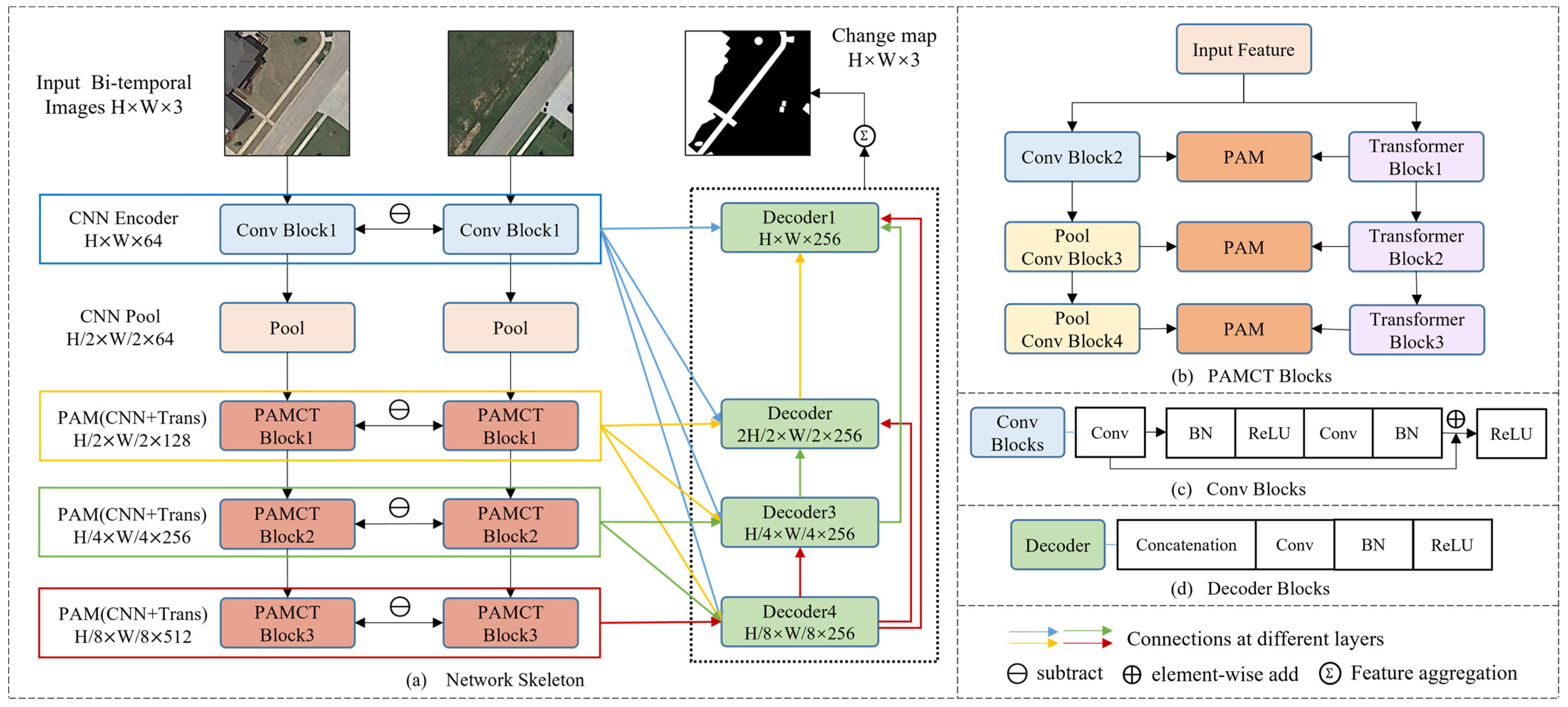
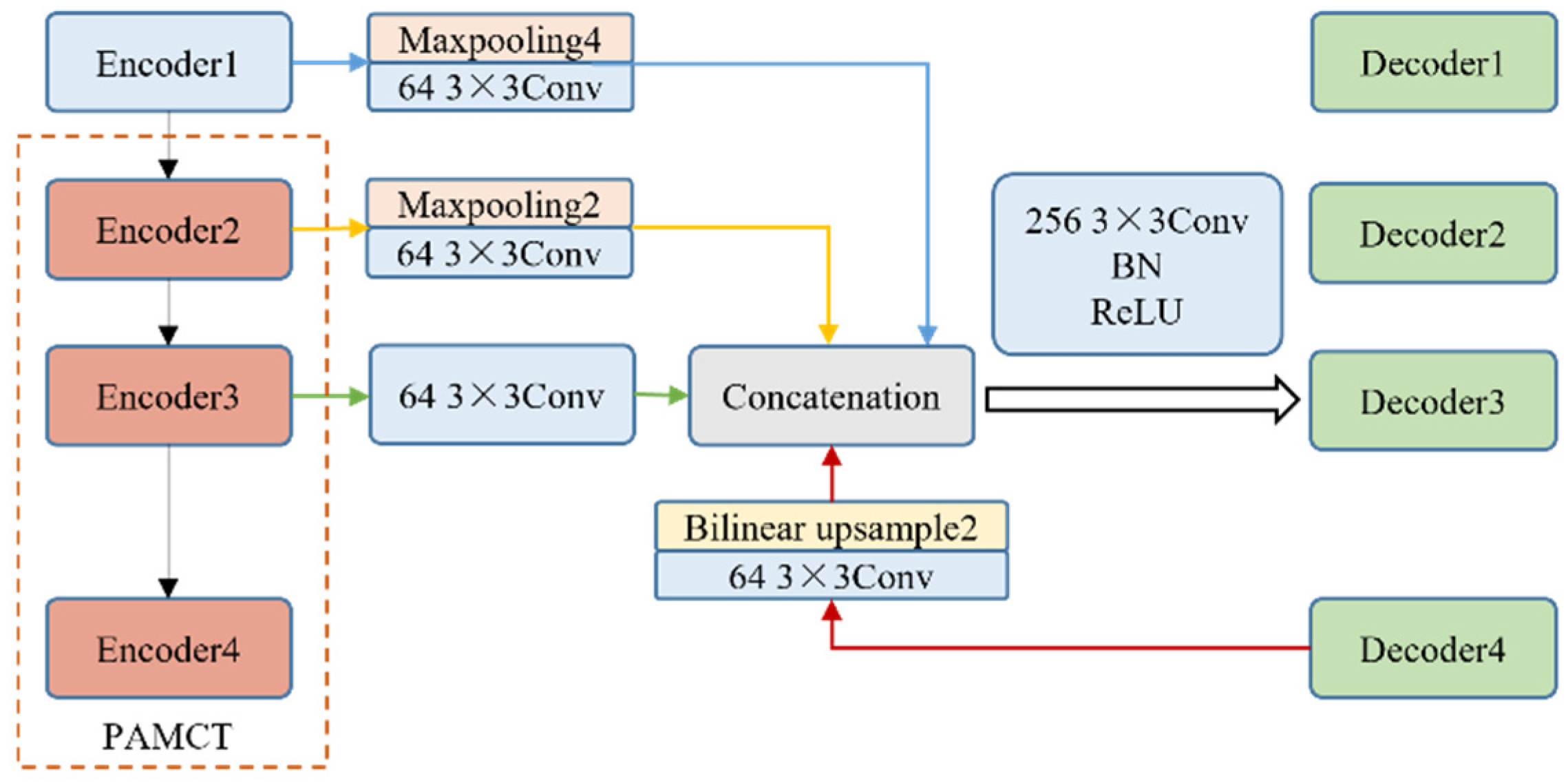
SUT is a standard U-shaped network using a Siamese structure as the encoder. The overall architecture of SUT consists of four symmetric encoders and decoders, as displayed in Figure 1. It takes dual temporal images as inputs to the Siamese network and shares parameters to enable the dual branch encoder to focus on the same area during feature extraction. The input images are first subjected to a convolutional block and then down-sampled once, as displayed in Figure 1c, which preserves the shallow information extracted using the CNN and reduces computational complexity. The subsequent three layers of encoders use PAM to fuse features generated from the CNN and transformer structures, fully leveraging the advantages of both structures and complementing each other, denoted as PAMCT. Here, the subtraction method is directly used to extract change maps between two Siamese branches, and the weight values are shared and connected to the decoder.

For the decoder, the inputs for each layer are four features generated in different scales. Considering the unidirectionality of information flow in the encoding process, full-scale skip connections are used to connect different levels of change maps to the decoder, which achieves multi-directional information flow and multi-scale feature fusion. Finally, SUT aggregates and classifies the outputs of each decoder layer to obtain the ultimate change features.

3.2. Encoder

Considering the computational complexity and feature extraction capability, the encoder is designed as a combination of a one-layer CNN and three-layer CNN–Transformer, as shown in Figure 2.

There are basic blocks, such as pooling operations, up-sample, conv blocks, transformer blocks, and PAMCT, in the encoder. The pool is the maximum pooling operation, and the up-sample blocks are designed to scale the feature images extracted using the CNN and transformer blocks to the same size during computation.

In Figure 1c, the calculation of conv blocks could be represented using Equation (1).

$$C_{ti}^k=\rho \left(BN\right(v_3\left(\rho \right(BN\left({v_3(F}_{ti}^k\right)\left)\right)\left)\right)+{v_3(F}_{ti}^k\left)\right)$$

(1)

where $F_{ti}^k$ represents the input feature map of layer $k (k=\mathrm{1,\; 2},\mathrm{3,\; 4})$ and the time phase $ti (i=\mathrm{1,2})$, $v_3$ represents $3\times 3$ convolution operations, $BN$ represents batch normalization, and $\rho$ represents the ReLU activation function.

3.3. Transformer Blocks

The output of the first CNN layer passes through the pooling and is inputted into the last three layers of the encoder. In the structure of the integrated CNN and transformer, the CNN also uses the conv blocks mentioned above, and the detailed transformer structure we used is displayed in Figure 3.

Before encoding with the transformer, the input images must proceed through patch embedding to be expanded into image sequences with tokens of shape $HW\times C$. Here, we set $T_l$ as the tokens after passing through the patch embedding, and these are calculated using Equation (2).

$$T_l=reshape\left(Flatten\right(x·W^D\left)\right)$$

(2)

where $x$ means the input images, $Flatten(·)$ represents a dimensionality reduction function, $W^D$ represents the weight matrixes of the deep convolution operation, and $reshape(·)$ represents the data reconstruction operation. Equation (2) actually represents data transformation in code and can be described as $(B,C,H,W)\to (B,HW,C)$, where $H$ and $W$ represent the image size, $C$ is the number of channels, and $B$ is the batch size during training.

The next module in the transformer is the self-attention module. When inputted into the self-attention module, tokens must first go through layer normalization [57]. Then, each layer uses a linear projection to produce three vectors Q, K, and V, which can be expressed using Equation (3).

$$\left\{\begin{array}{c}Q=T_l·W_l^q\\ K=T_l·W_l^k\\ V=T_l·W_l^v\end{array}\right.$$

(3)

where $T_l$ represents the tokens of the layer, $W_l^q$, $W_l^k$, and $W_l^v$ represent learnable parameters. Besides, $Q$, $K$, and $V$ of the same layer have the identical $HW\times C$ dimension. After obtaining the Q, K, and V vectors, self-attention can be described using Equation (4) [47].

$$Attention\left(Q,K,V\right)=softmax\left(\frac{Q{K}^T}{\sqrt{d_{head}}}\right)V$$

(4)

where $softmax(·)$ is a softmax function along the channel dimension and $d_{head}$ is the channel dimension of the head in the $Q/K/V$ vector.

Furthermore, the core structure of the transformer is multi-head self-attention (MSA). MSA divides Q, K, and V vectors into multiple separate heads, computes the attention coefficient of each head, and then concatenates their values. This process can be described using Equations (5) and (6).

$${\mathrm{h}\mathrm{e}\mathrm{a}\mathrm{d}}_j\left(T_l\right)=Attention(T_l·W_l^q,T_l·W_l^k,T_l·W_l^v)$$

(5)

$$MSA\left(T_l\right)=Concat\left({\mathrm{h}\mathrm{e}\mathrm{a}\mathrm{d}}_1\right(T_l),\cdots ,{\mathrm{h}\mathrm{e}\mathrm{a}\mathrm{d}}_n(T_l\left)\right)W^o$$

(6)

where ${\mathrm{h}\mathrm{e}\mathrm{a}\mathrm{d}}_j(·)$ is the multiple independent heads, with $j$ taking values between 1 and n, $Concat(·)$ represents a concatenation operation, $W^o$ means a matrix for linear projection, and $n$ is the number of heads.

We perform layer normalization on the output of MSA and compute it through MLP to obtain the output features of the transformer. The MLP in the transformer mainly comprises two linear projection layers, with one of the projection transformations using the GELU activation function [58]. The implementation of MLP is expressed in Equation (7).

$$MLP\left(T_l\right)=GELU\left(T_l·W^1\right)·W^2$$

(7)

where $W^1$ and $W^2$ represent learnable linear projection matrices that can expand and compress the channel dimensions of tokens.

After the process shown in Figure 3, we can obtain the 2D feature maps $F_{ti}^{global}$ containing rich global contextual information, and it is also necessary to convert $F_{ti}^{global}$ into images that match the shape of the input images, which is the process $(B, HW, C) \to (B, C, H, W)$, in order to facilitate subsequent feature fusion between the CNN and transformer.

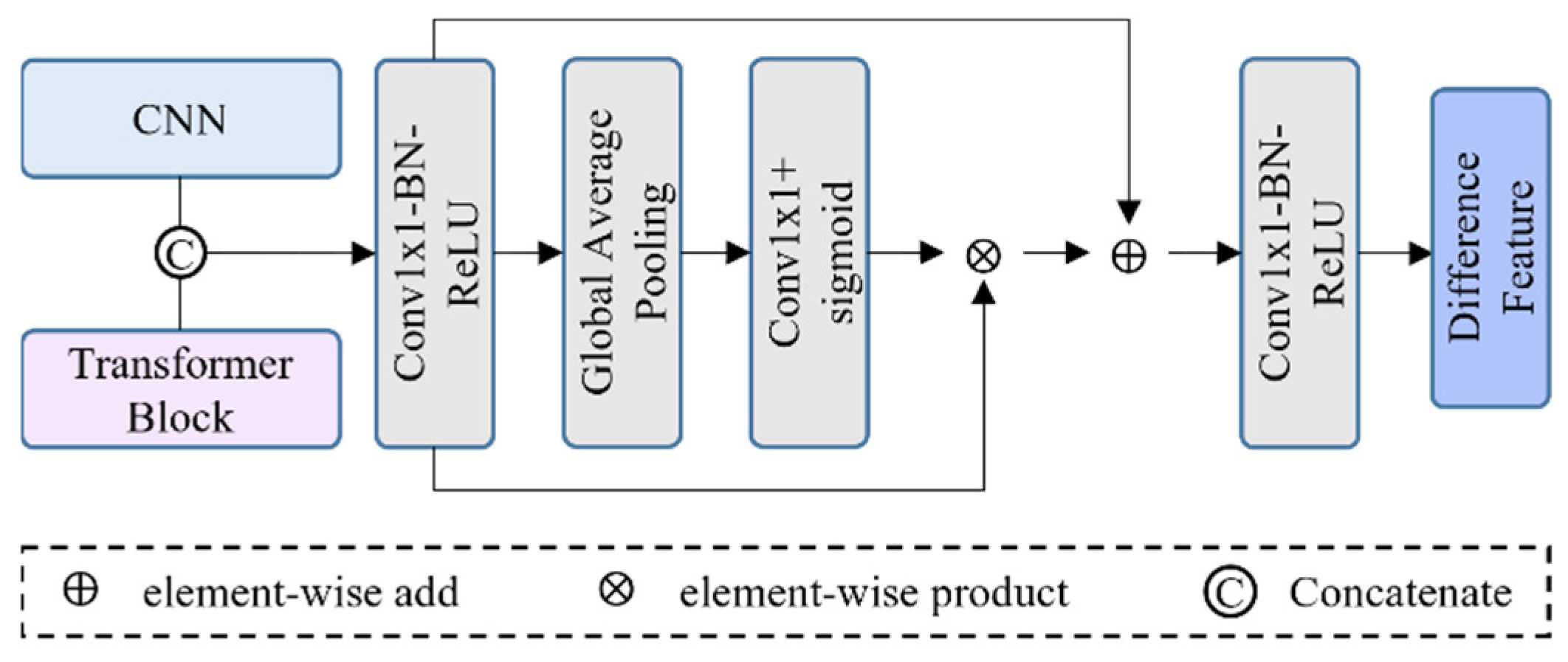
3.4. PAMCT Blocks and PAM Module

The composition of PAMCT is displayed in Figure 1b, which is designed to fuse feature maps extracted from the CNN and transformer using the PAM [31,59]. The calculation process of the PAM is shown in Figure 4.

The PAM takes the features generated from the CNN and transformer as inputs, concatenates them, and enhances the change features through channel attention. As displayed in Figure 4, the feature maps undergo global average pooling after convolution and are activated with sigmoid, while introducing residual connections to improve performance. Finally, the PAM adopts a $1\times 1$ convolution to obtain the output feature. The mathematical expression of the calculation process of the PAM is shown in Equations (8) and (9).

$$A_{ti}^k=\rho \left(BN\right(v_1\left(Concat\right(C_{ti}^k,T_{ti}^k\left)\right)\left)\right)$$

(8)

$$F_{ti}^k=A_{ti}^k\ast \sigma \left(v_1\right(GAP\left(A_{ti}^k\right)\left)\right)+A_{ti}^k$$

(9)

where $C_{ti}^k$ and $T_{ti}^k$, respectively, denote the features extracted using the k-th $(k=\mathrm{2,\; 3},4)$ layer of the CNN and transformer at time $ti(i=\mathrm{1,\; 2})$, $Concat(·)$ denotes the concatenation operation, $v_1$ denotes $1\times 1$ convolution, $BN$ denotes batch normalization, $\rho$ denotes the ReLU activation function, $GAP(·)$ denotes the global average pooling, $\sigma$ denotes a sigmoid function, and the output feature of PAM is $F_{ti}^k$.

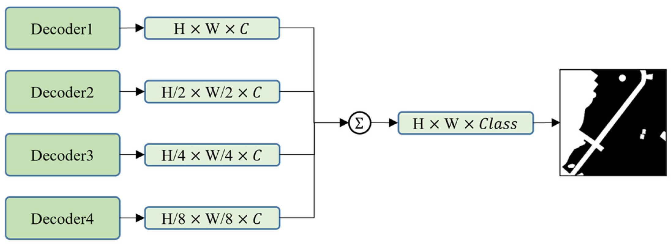
3.5. Decoder with Full-Scale Skip Connection

Currently, transformer-based networks connect the encoder and decoder layer-by-layer for inter-scale communication, resulting in unidirectional information flow and the easy loss of feature information. In response to this issue, this study was inspired by [32,33] and adopted full-scale skip connections to achieve multi-scale information flow in multiple directions while maintaining high-resolution and fine-grain feature representations. Considering the encoder structure and computational limitations, we adopt a four-layer decoder to achieve full-scale skip connections. The structure of the third layer decoder is taken as an example, as displayed in Figure 5.

This process can be described as the maximum pooling of the change maps in Encoder1 and Encoder2 to the size of the change map in Encoder3, then up-sampling the output features of Decoder4 to the size of the change map in Encoder3, concatenating the above features with the change map in Encoder3, and finally fusing them through convolution to attain the output feature of Decoder3. This process can be described using Equations (10)–(12).

$${En}^k=abs(F_{t1}^k-F_{t2}^k)$$

(10)

$$F^3=Concat\left(v_3\right(M_4\left({En}^1\right),M_2\left({En}^2\right),{En}^3,U_2\left({De}^4\right)\left)\right)$$

(11)

$${De}^3=\rho \left(BN\right(v_3\left(F^3\right)\left)\right)$$

(12)

where $F_{t1}^k$ and $F_{t2}^k$ are the bi-temporal features of the k-th layer $(k=\mathrm{1,\; 2},\mathrm{3,\; 4})$, ${En}^k$ is the output change map of each encoder layer, and $abs(·)$ is the absolute value difference. $Concat(·)$ means the concatenating operation, $M_2$ and $M_4$ denote maximum pooling with coefficients of $\mathrm{½}$ and $1/4$, $U_2$ represents up-sampling to twice the size, $v_3$ represent convolution with a $3\times 3$ kernel, $BN$ means batch normalization, and $\rho$ represents the ReLU activation function.

Other layers of decoders can be obtained using similar calculations. Last, the outputs of the decoder at different scales are fused after being deep supervised, and the final feature maps are what we need, as shown in Figure 6.

3.6. Loss Function

In the remote sensing image change detection, the quantity of pixels that have not changed is much greater than the quantity of pixels that have changed. In this study, we adopt a mixed weighted loss function to alleviate the problem of sample imbalance. Here, we consider the mixed method of weighted cross-entropy loss [46] and dice loss [60], so the loss function can be expressed using Equation (13).

$$L=L_{wce}+L_{dice}$$

(13)

where $L_{wce}$ represents the weighted cross-entropy loss, $L_{dice}$ represents the dice loss, and $L$ is the loss function we used.

Cross-entropy can be defined as Equation (14). Here, we set $P$ as the real probability distribution, $Q$ is the predicted probability distribution, and $x_i$ refers to the probability of image pixel distribution.

$$H\left(P,Q\right)=-\sum _{i=1}^{n}P\left(x_i\right)\times \log \left(Q\right(x_i\left)\right)$$

(14)

When the sample label is binary {0, 1}, $P$ is taken as 0 or 1, $Q$ is taken as $\left(\mathrm{0,1}\right]$ after softmax, and if we define $R$ as the probability of correct the prediction, the cross-entropy can be optimized using Equation (15).

$$H\left(P,Q\right)=-\log \left(R\right(x_i\left)\right)$$

(15)

Moreover, $L_{wce}$ can use the coefficient ${\alpha }_t$ to show the importance of the sample in the loss, strengthening the contribution of changed pixels and reducing the contribution of unchanged pixels to the loss function, thus to some extent alleviating the sample imbalance problem, as shown in Equation (16). The coefficient ${\alpha }_t$ can be defined using Equation (17) [46].

$$L_{wce}=-{\alpha }_t\log \left(R\right(x_i\left)\right))$$

(16)

$${\alpha }_t=\frac{1}{H\times W}\sum _{k=1}^{H\times W}weight\left[class\right]$$

(17)

where the value of $class$ is 0 or 1, which indicates non-changed or changed pixels, and H and W means the size of the change maps.

Dice loss is a metric function used to evaluate the similarity between samples. It can curb the problem of positive and negative samples being strongly imbalanced. The range of dice loss is [0, 1], and the larger the value, the more similar the samples. The calculation of dice loss can be defined using Equation (18).

$$L_{dice}=1-\frac{\left|P\right(x_i)\bigcap softmax(Q\left(x_i\right)\left)\right|}{\left|P\left(x_i\right)\right|+\left|softmax\right(Q\left(x_i\right)\left)\right|}$$

(18)

4. Experimental Results and Analysis

In this section, we introduce the datasets, experimental settings, and evaluation metrics, then in detail, show the performance of SUT based on three public datasets, and compare it with the state-of-the-art methods to demonstrate its efficiency. Moreover, an ablation experiment is designed to verify the effectiveness of the blocks used in SUT.

4.1. Datasets

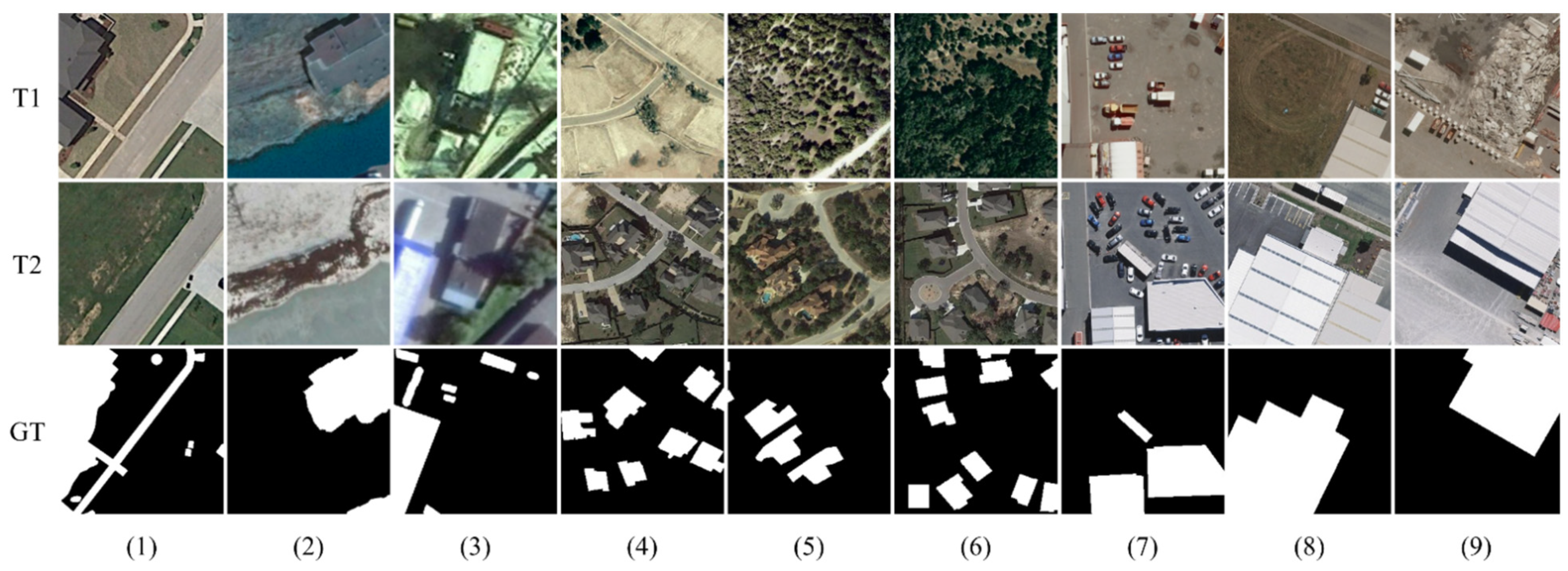
Three remote sensing image datasets that we used, namely CDD [43], LEVIR-CD [24], and WHU-CD [61], are adopted to verify the performance of the proposed network, as shown in Figure 7.

CDD dataset: a remote sensing image set with significant seasonal changes and various sizes of changed classes, such as buildings, roads, cars, etc. The images in this dataset are RGB images with a spatial resolution from 3 to 10 cm per pixel. And there are 16,000 pairs of dual temporal non-overlapping images of 256 × 256 pixels in size. The quantity of training, validation, and testing sets in CDD are 10,000, 3000, and 3000 pairs, respectively.

LEVIR-CD dataset: a building CD dataset collected from Texas, USA. It is an RGB image dataset with a spatial resolution of 0.5 cm per pixel. The size of the images in LEVIR-CD is $1024\times 1024$ pixels. There are a total of 637 pairs of images in it. The training, validation, and testing datasets are 445 pairs, 64 pairs, and 128 pairs of images, respectively. Since the image size is large, and if the image pairs are used directly for training, it would lead to excessive memory consumption. Therefore, they need to be cropped into non-overlapping image pairs of $256\times 256$ pixels in advance, and correspondingly the training, validation, and test datasets are 7120, 1024, and 2048 image pairs, respectively.

WHU-CD dataset: a city-building CD dataset with bi-temporal high-resolution (0.075 m/pixel) remote sensing images collected from the Christchurch, New Zealand, region by Wuhan University. Similarly, considering the required memory, the images in WHU-CD are cropped into non-overlapping image pairs of $256\times 256$ pixels in size, and the training, validation, and test datasets consist of 6096, 762, and 762 image pairs, respectively.

4.2. Implementation Details

All experiments in this study were carried out using the Ubuntu 22.04 operating system, with the deep learning framework of Pytorch, coded in Python, and trained, verified, and tested on the server equipped with multiple NVIDIA GeForce RTX 4090 graphics cards. In terms of the model architecture, SUT adopts a four-layer encoder, with the last three layers using a fusion structure of the CNN and transformer. And on the Siamese structure, we use subtraction to connect the dual temporal phase diagram. In addition, the sampling strategy is 1/2 of the last-layer image size in the transformer settings. In the training process based on the three datasets, the SUT network adopts Adam as the optimizer and employs a cosine annealing learning rate as the adjustment strategy, which sets the initial learning rate to 1 × 10⁻⁴ and the minimum learning rate to 1 × 10⁻⁶. In addition, all experiments set the batch size to 8, and 200 epochs are trained for each dataset.

4.3. Evaluation Metrics

The aim of CD is to detect changing and non-changing pixels, which is a binary classification problem in essence. Therefore, the following classification evaluation indicators can be used for the accuracy evaluation: Precision, Recall, F1-score, IOU, and overall accuracy (OA). The calculation for these indicators can be described using Equations (19)–(23), where TP means true positive, TN means true negative, FN means false negative, and FP means false positive.

$$Precision=\frac{TP}{TP+FP}$$

(19)

$$Recall=\frac{TP}{TP+FN}$$

(20)

$$F1=\frac{2\times Precision\times Recall}{Precision+Recall}$$

(21)

$$IOU=\frac{TP}{TP+FP+FN}$$

(22)

$$OA=\frac{TP+TN}{TP+TN+FP+FN}$$

(23)

4.4. Comparative Methods

To verify the superior performance of our method SUT, we contrast it with some state-of-the-art methods as follows:

(1)

FC-Siam-Diff [39]: The network architecture is Siamese Unet. And it is a CNN-based network that uses the feature difference to generate change information from dual temporal images.

(2)

RDPnet [62]: It is a CNN-based network that uses an efficient training strategy to make CNNs learn from easy to hard and proposes an edge-constrained loss function to enhance the extraction of boundary details.

(3)

Bit [25]: It is a transformer-based network. It first extracts semantic features through CNN, then proceeds to global modeling with a transformer, strengthening the contextual information of the change features.

(4)

ChangeFormer [27]: The network only adopts the transformer structure and achieves CD tasks through a Siamese transformer encoder and an MLP decoder.

(5)

SiUnet3+-CD [33]: It is a CNN-based network using a full-scale connected Siamese Unet3+ network to extract features.

(6)

SNUnet-CD [46]: It uses a densely connected Siamese Unet++ network to extract change features and fuses four levels of features of different sizes using the ECAM.

(7)

MCTnet [30]: It considers the characteristics of the CNN and transformer and adopts the Siamese Unet structure to fuse the features extracted using the CNN and transformer through an attention mechanism.

The parameters of the above method were set based on the results of the original research. If the parameters of any method are not mentioned in the original study, we optimized them as much as possible. In addition, because the code of MCTnet and SiUnet3+-CD are not publicly available, we reproduced them ourselves.

4.5. Results and Analysis

We have trained the proposed SUT and the comparative methods based on the CDD, LEVIR-CD, and WHU-CD datasets, with their respective best results obtained from multiple training sessions being compared, and multiple cross-validation experiments were conducted based on hyperparameter settings to protect against overfitting. To highlight the importance of change information and the weakened impact of non-change information, all methods only evaluate the accuracy of change information based on the test set.

Table 1. Quantitative results of various methods based on the CDD dataset. The best results are bolded and underlined, while the second-best results are bolded.

Methods/Channel	Pre (%)	Rec (%)	F1 (%)	IOU (%)	OA (%)
FE-Siam-diff/32 (2018)	82.96	62.11	71.04	55.08	93.84
RDPnet/- (2022)	96.45	89.39	92.78	86.54	98.31
Bit/- (2021)	95.74	88.03	91.72	84.72	98.07
ChangeFormer/- (2022)	95.87	90.27	92.99	86.90	98.34
SiUnet3+-CD/64 (2022)	97.23	89.64	93.28	87.41	98.43
SNUnet-CD/64 (2021)	96.71	92.01	94.30	89.21	98.71
MCTnet/64 (2022)	97.85	91.02	94.31	89.23	98.78
SUT/64 (ours)	97.98	91.67	94.71	89.95	98.93

displays the quantitative results of all methods based on the CDD dataset. The SUT method we proposed performs excellently, realizes the best results in precision (97.98%), F1 (94.71%), IOU (89.95%), and OA (98.93%). The worst performance is achieved using the FE-Siam-diff network, which only adopts a simple Siamese Unet with an all-convolutional structure. It has poor feature extraction capability, making it difficult to capture the features associated with large seasonal changes. RDPnet, due to its efficient sampling strategy and edge-loss, has made strides in detecting edge features, yet it has issues with smoothing linear changing features. SNUnet-CD fully used the advantages of dense connection and the ECAM, achieving the highest recall rate, but it was not detailed enough in detecting boundary and linear targets. The SiUnet3+-CD network performs well with good quantitative indicators, demonstrating the effectiveness of full-scale skip layer connections. However, its overly complex calculations have led to missed detections based on small targets and boundary features. Although Bit and ChangeFormer have good global modeling capabilities, there are problems with the excessive smoothing of boundaries and corners. As for MCTnet lacking in linear change feature detection, it is slightly lower than SUT based on multiple evaluation indicators, and its concise structure of combining a CNN and transformer confirms the powerful performance of CNNs fused with transformers. 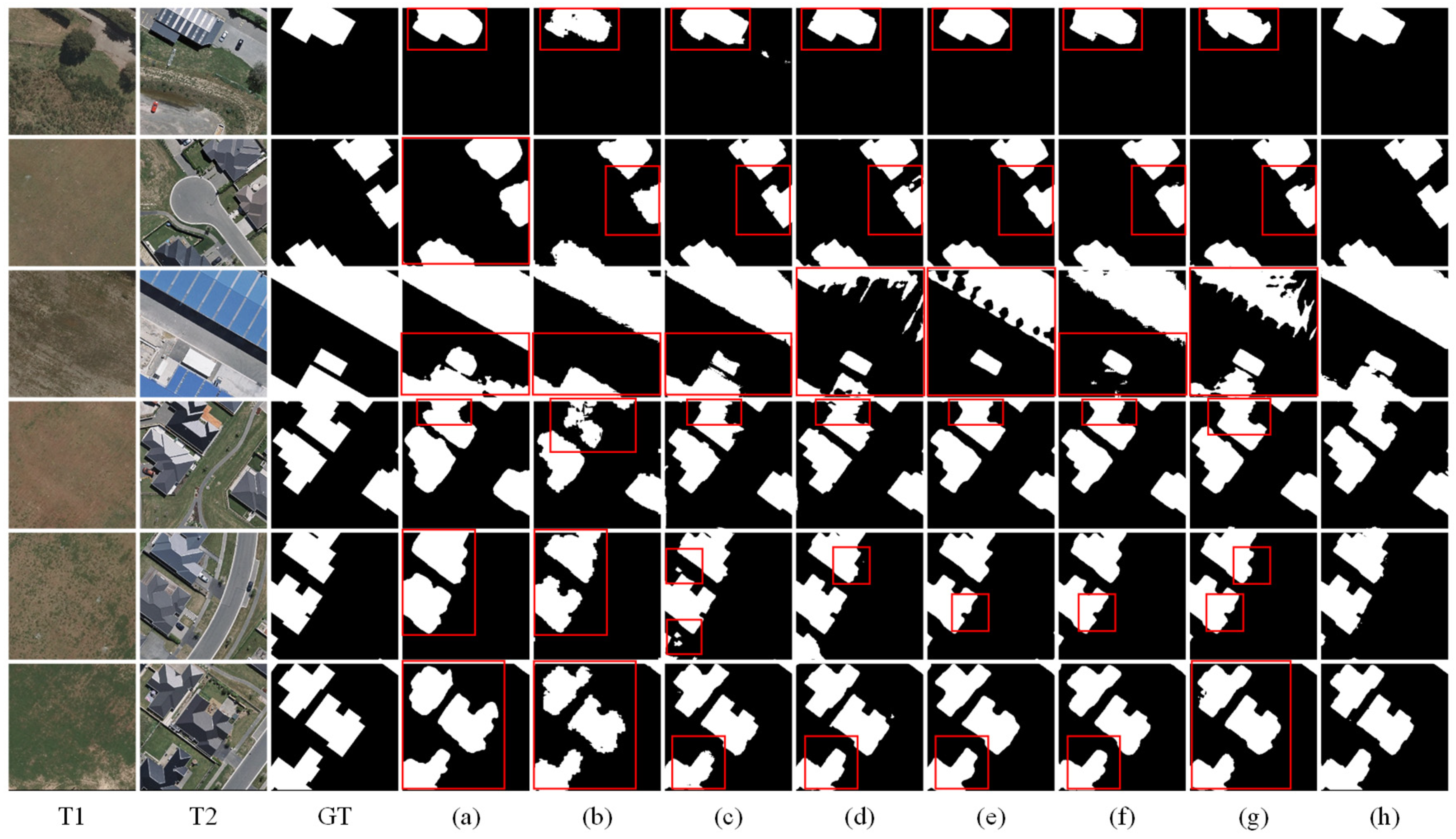Figure 8 displays the visualization results of the CD on the CDD dataset as a sample. Compared with other methods, SUT performs the best in detecting contour integrity and accuracy and can effectively weaken the effects of factors, such as lighting and seasonal changes.

Table 2. Quantitative results of various methods based on the LEVIR-CD dataset. The best results are bolded and underlined, while the second-best results are bolded.

Methods/Channel	Pre (%)	Rec (%)	F1 (%)	IOU (%)	OA (%)
FE-Siam-diff/32 (2018)	87.91	85.31	86.59	76.35	98.65
RDPnet/- (2022)	89.29	86.59	87.92	78.44	98.79
Bit/- (2021)	91.70	89.72	90.70	82.98	99.06
ChangeFormer/- (2022)	92.21	88.77	90.46	82.58	99.05
SiUnet3+-CD/64 (2022)	92.37	89.58	90.95	83.41	99.09
SNUnet-CD/64 (2021)	91.99	90.46	91.22	83.86	99.11
MCTnet/64 (2022)	92.70	89.13	90.88	83.28	99.08
SUT/64 (ours)	92.82	90.25	91.52	84.36	99.14

shows the performance of various methods based on the LEVIR-CD dataset. SUT performs well, achieving the best results in Precision (92.82%), F1 (91.52%), IOU (84.36%), and OA (99.14%). The accuracy of FE-Siam-diff is slightly poor, and its test results often feature cavities. RDPnet still has troubles with missed and false detections, and the feature boundaries are not smooth. Due to their dense connections, SNUnet-CD and SiUnet3+-CD have quite good quantitative indicators and complete contours, but there are many small target misdetections. In addition, Bit suffers from the missed and false detection of small targets and has overly smooth contours. ChangeFormer has fewer instances of false positives but performs poorly based on edge information, making it prone to unevenness and blurriness. MCTnet performs mediocrely in building CDs, with frequent occurrences of false positives and edge blurring. Figure 9 shows a sample of the visualization results for CD in the LEVIR-CD dataset. Upon comparing SUT with the other networks, it is not difficult to confirm that SUT can better suppress false and missed detections. It is outstanding in extracting the contour of change features, which is especially suitable for detecting regular ground change features, such as buildings.

Among the three datasets, the WHU-CD has the smallest number of samples, and the training effect is relatively unstable. After multiple training sessions, the result with a minimum loss during the iteration is used for the quantitative comparison in this experiment. As shown in

Table 3. Quantitative results of various methods based on the WHU-CD dataset. The best results are bolded and underlined, while the second-best results are bolded.

Methods/Channel	Pre (%)	Rec (%)	F1 (%)	IOU (%)	OA (%)
FE-Siam-diff/32 (2018)	63.49	88.29	73.86	58.56	97.44
RDPnet/- (2022)	93.78	77.23	84.70	73.46	98.86
Bit/- (2021)	95.84	77.38	85.63	74.87	98.94
ChangeFormer/- (2022)	93.51	80.15	86.31	75.92	98.96
SiUnet3+-CD/64 (2022)	92.82	77.53	84.49	73.14	98.83
SNUnet-CD/64 (2021)	89.04	80.70	84.67	73.41	98.81
MCTnet/64 (2022)	93.41	79.53	85.91	75.30	98.94
SUT/64 (ours)	93.83	88.07	90.84	82.83	99.29

, SUT still obtains the best results in F1 (90.61%), IOU (82.83%), and OA (99.26%), which has the best comprehensive performance. The best Precision (95.84%) is obtained by Bit, which uses CNN to simply connect the transformer, making the edges smoother. However, when detecting changes in buildings with larger targets, holes are prone to occur in Bit, similar to ChangeFormer. The best Recall (88.29%) is achieved by FE-Siam-diff, which performs well based on simple datasets with a weak seasonal effect, but with a rudimentary structure; its detection performance is not satisfactory, leading to problems of false detection. For RDPnet, it performs well in detecting large targets, but there is a problem with irregular boundaries for small targets. The calculation of SiUnet3+-CD is too complex, often missing portions when detecting large target changes in buildings. SNUnet-CD rarely misses detections, but it lacks global modeling capabilities and is prone to issues, such as false detections of small targets in the WHU-CD dataset. MCTnet may perform poorly in contour extraction due to an insufficient connection between the CNN and transformer at different scales. As shown in Figure 10, SUT has better detection ability based on change targets of different sizes than the above methods and has smooth boundaries and regular contours.

From the experiments, it can be seen that SUT achieves the best performance based on the three datasets. The extracted results of SUT based on boundaries, linear targets, and small targets are more detailed than other methods. In addition, as the number of samples in the dataset decreases, the abovementioned advantages of SUT become more apparent.

4.6. Channel Hyperparameter Adjustment

This study takes channel dimensions in the feature map of the network as an adjustable hyperparameter. The comparative experiments mentioned above are conducted by setting the adjustable channel dimensions to 64n $(n=\mathrm{1,\; 2},\mathrm{3,\; 4}\dots )$ while retaining the original network parameters. Therefore, in order to verify that SUT can maintain its excellent performance even with a smaller channel dimension, a comparative experiment with 32 channels was conducted.

As shown in

Table 4. Accuracy results of channel hyperparameter comparison experiment. The best results are bolded and underlined, while the second-best results are bolded.

Method/Channel	F1 (%)	IOU (%)	OA (%)
	CDD
FE-Siam-diff/32 (2018)	71.04	55.08	93.84
RDPnet/- (2022)	92.78	86.54	98.31
Bit/- (2021)	91.72	84.72	98.07
ChangeFormer/- (2022)	92.99	86.90	98.34
SiUnet3+-CD/64 (2022)	93.28	87.41	98.43
SNUnet-CD /32 (2021)	92.65	86.60	98.32
MCTnet/32 (2022)	93.24	87.34	98.41
SUT/32 (our)	93.57	87.91	98.49
	LEVIR-CD
FE-Siam-diff/32 (2018)	86.59	76.35	98.65
RDPnet/- (2022)	87.92	78.44	98.79
Bit/- (2021)	90.70	82.98	99.06
ChangeFormer/- (2022)	90.46	82.58	99.05
SiUnet3+-CD/64 (2022)	90.95	83.41	99.09
SNUnet-CD /32 (2021)	90.97	83.44	99.09
MCTnet/32 (2022)	90.16	82.09	99.02
SUT/32 (our)	91.05	83.57	99.11
	WHU-CD
FE-Siam-diff/32 (2018)	73.86	58.56	97.44
RDPnet/- (2022)	84.70	73.46	98.86
Bit/- (2021)	85.63	74.87	98.94
ChangeFormer/- (2022)	86.31	75.92	98.96
SiUnet3+-CD/64 (2022)	84.49	73.14	98.83
SNUnet-CD /32 (2021)	81.12	68.24	98.60
MCTnet/32 (2022)	83.23	71.28	98.78
SUT/32 (our)	87.23	77.35	99.01

, from the accuracy perspective, SUT also has the best comprehensive performance when using 32 channels, achieving the best F1, IOU, and OA results based on all three datasets. Significantly, SUT with 32 channels is already superior to FE-Siam-diff, Bit, ChangeFormer, and SiUnet3+-CD with their optimal settings from the corresponding publications. In addition, SNUnet-CD and MCTnet are indeed better at 64 channels than SUT at 32 channels. However, when both are set to the same channel dimension, SUT performs better than SNUnet-CD and MCTnet. In summary, SUT definitely maintains good CD ability even with 32 channels and performs best among the compared networks.

4.7. Efficiency Evaluation

Furthermore, the efficiency of models also needs to be considered. Efficiency represents the computational complexity and memory cost during model training and prediction, and there is a bounded relationship between efficiency and accuracy in deep learning methods. Therefore, we compared the Parameters, Flops, and Time of the above methods, based on the input datasets using image sizes of 256 × 256 pixels and training parameter settings, shown in

Table 5. Comparison of Parameters, Flops, and Time of different methods under the same settings.

Method/Channel	Parameters (M)	Flops (G)	Time (MS)
FE-Siam-diff/32	5.39	18.66	11.23
RDPnet/-	1.69	27.12	23.32
SNUnet-CD/32	10.20	44.38	13.09
SNUnet-CD/64	40.77	176.33	22.42
SiUnet3+-CD/64	27.23	217.61	33.68
Bit/-	3.04	9.88	23.56
ChangeFormer/-	41.03	202.79	51.72
MCTnet/32	10.12	22.51	47.58
MCTnet/64	40.24	88.94	48.35
SUT/32 (ours)	9.87	40.43	42.31
SUT/64 (ours)	39.18	159.62	47.43

. Parameters refer to the quantity of parameters used in the model, Flops refers to the calculation amount of the model, and Time means the reaction time cost of the model to deal with a single image. Apparently, SUT performs well in terms of Parameters and Flops while achieving the best overall results, and the Time is also within the reasonable range. When the channel number reaches 64, despite the performance degradation based on parameters and Flops, the effect of CD in SUT is further improved.

4.8. Ablation Studies

To demonstrate the effectiveness of the PAM fusion based on the CNN and transformer in SUT, as well as the effect of deep supervision and the Unet3+ structure, we conducted ablation experiments based on the CDD, LEVIR-CD, and WHU-CD datasets. For the sake of the comparison, we refer to the network that does not use deep supervision and the PAM as SUT-base, the network that only uses deep supervision without the PAM as SUT-sup, the network that only uses the PAM without deep supervision as SUT-PAM, the network that uses both the PAM and deep supervision as SUT-PAM-sup, and the network that uses the Unet structure with the transformer, PAM, and deep supervision as UnetT-PAM-sup.

Table 6. Ablation experiments based on the CDD dataset. The best results are highlighted in bold font.

Method	Pre (%)	Rec (%)	F1 (%)	IOU (%)	OA (%)
SUT-base	96.74	89.74	93.11	87.11	98.39
SUT-sup	95.63	89.09	92.24	85.61	98.18
SUT-PAM	97.24	91.22	94.13	89.19	98.76
SUT-PAM-sup	97.98	91.67	94.71	89.95	98.93
UnetT-PAM-sup	97.04	90.33	93.56	87.91	98.49

,

Table 7. Ablation experiments based on the LEVIR-CD dataset. The best results are highlighted in bold font.

Method	Pre (%)	Rec (%)	F1 (%)	IOU (%)	OA (%)
SUT-base	92.64	89.17	90.87	83.27	99.07
SUT-sup	92.59	89.34	90.93	83.37	99.08
SUT-PAM	92.90	89.85	91.35	84.08	99.13
SUT-PAM-sup	92.82	90.25	91.52	84.36	99.14
UnetT-PAM-sup	92.45	87.88	90.11	83.11	98.89

and

Table 8. Ablation experiments based on the WHU-CD dataset. The best results are highlighted in bold font.

Method	Pre (%)	Rec (%)	F1 (%)	IOU (%)	OA (%)
SUT-base	85.37	85.85	85.61	74.84	98.82
SUT-sup	91.16	88.73	89.93	81.70	99.19
SUT-PAM	86.65	88.33	87.48	77.75	98.97
SUT-PAM-sup	93.30	88.07	90.61	82.83	99.26
UnetT-PAM-sup	92.51	84.33	88.23	81.12	98.97

display the quantitative results of these ablation experiments based on the CDD, LEVIR-CD, and WHU-CD datasets. From these tables, we can find that the best results are all achieved in SUT-PAM-sup. the results obtained by the networks with the PAM are obviously better than those of the networks without the PAM, which indicates that the PAM has a significant impact on the integration of CNN and transformer structures. In addition, the results of the networks with deep supervision show that as the number of samples in the dataset decreases, the effectiveness of deep supervision gradually improves. Moreover, when we change the backbone of the SUT from Unet3+ to Unet, it is obvious that the CD effect is not as good as the original structure.

Some example outputs of the ablation studies based on the three datasets are displayed in Figure 11(a1–e1). Specifically, in SUT, deep supervision can suppress the occurrence of falsely detected small targets, as shown in Figure 11(5) and (7), and reduce the problem of concave holes at the boundary of changed targets, as shown in Figure 11(1), (8) and (9). The methods with the PAM have better performance based on linear targets and contour optimization, as shown in Figure 11(2), (3) and (9). Furthermore, regarding corner details, the results of networks with the PAM are closer to the GT than those without the PAM. It is demonstrated that the PAM contributes to the fusion of the CNN and transformer. As shown in Figure 11(e1) for the SUT method under the Unet architecture, comparing the results of the Unet3+ and Unet structures, it can be seen that the advantages of Unet3+ are specifically in the linear target integrity and the suppression of the misdetection of small targets. We also utilized a heatmap to visualize the results of the above ablation experiments, as shown in Figure 11(a2–e2). Based on a thermal comparison, it can be found that SUT significantly improved feature extraction while using the PAM, Unet3+ structure, and deep supervision. We can compare Figure 11(a2,b2) and Figure 11(c2,d2) and find that deep supervision does have a role in optimizing the boundaries and enhances the detection of changing targets to some extent in the heat map. And when comparing Figure 11(a2,c2) and Figure 11(b2,d2), we can find that the results of detecting the linearly changing targets are related to whether or not the PAM structure is used, and in general, it seems that the network fusing the CNN and the transformer by the PAM performs better. As for the backbone network of Unet3+ and Unet, it is easy to see that Unet3+ has a huge advantage in detecting the changing target integrity from the heat map.

5. Conclusions

In this study, we propose a full-scale connected CNN–Transformer network named SUT for the CD of remote sensing images. The network encoder comprises a one-layer CNN and a three-layer integrated CNN and transformer. In response to the lack of global modeling abilities of CNNs, the boundary generalization of pure transformer networks, and the problem of potentially omitting small targets when CNNs are connected to transformers, this study adopts the PAM to effectively fuse CNN and transformers. Furthermore, to address the problem of detail feature loss due to inter-scale communication and one-way information flow in the existing networks that fuse CNNs and transformers, we apply full-scale skip connections for the encoder and decoder. The comparative experiments based on public datasets demonstrate the effectiveness of the proposed SUT. Specifically, it performs well in restoring the shape of changed targets, with clear and complete detailed features, such as contours, corners, and linear targets. However, the change detection effect of SUT training based on fewer samples is unsatisfactory. One of our possible future works is to adopt the weakly supervised learning to address this problem.

References

1. Singh, A. Review article digital change detection techniques using remotely-sensed data. Int. J. Remote Sens. 1989, 10, 989–1003. [Google Scholar] [CrossRef]
2. Weng, Q. Land use change analysis in the Zhujiang Delta of China using satellite remote sensing, GIS and stochastic modelling. J. Environ. Manag. 2002, 64, 273–284. [Google Scholar] [CrossRef] [PubMed]
3. Peng, D.; Zhai, C.; Zhang, Y.; Guan, H. High-resolution optical remote sensing image change detection based on dense connection and attention feature fusion network. Photogramm. Rec. 2023, 11, 40–59. [Google Scholar] [CrossRef]
4. Zerrouki, N.; Harrou, F.; Sun, Y.; Hocini, L. A machine learning-based approach for land cover change detection using remote sensing and radiometric measurements. IEEE Sens. J. 2019, 19, 5843–5850. [Google Scholar] [CrossRef]
5. Liu, M.; Shi, Q.; Chai, Z.; Li, J. PA-Former: Learning prior-aware transformer for remote sensing building change detection. IEEE Geosci. Remote Sens. Lett. 2022, 19, 6515305. [Google Scholar] [CrossRef]
6. Adams, J.; Chandler, J. Evaluation of LIDAR and medium scale photogrammetry for detecting soft-cliff coastal change. Photogramm. Rec. 2002, 17, 405–418. [Google Scholar] [CrossRef]
7. Esposito, G.; Salvini, R.; Matano, F.; Sacchi, M.; Danzi, M.; Somma, R.; Troise, C. Multitemporal monitoring of a coastal landslide through SfM-derived point cloud comparison. Photogramm. Rec. 2017, 32, 459–479. [Google Scholar] [CrossRef]
8. Deng, G.; Pinoli, J.C. Differentiation-based edge detection using the logarithmic image processing model. J. Math. Imaging Vis. 1998, 8, 161–180. [Google Scholar] [CrossRef]
9. Malila, W.A. Change Vector Analysis: An Approach for Detecting Forest Changes with Landsat; Purdue University: West Lafayette, IN, USA, 1980; p. 385. [Google Scholar]
10. Ludeke, A.K.; Maggio, R.C.; Reid, L.M. An analysis of anthropogenic deforestation using logistic regression and GIS. J. Environ. Manag. 1990, 31, 247–259. [Google Scholar] [CrossRef]
11. Celik, T. Unsupervised change detection in satellite images using principal component analysis and k-means clustering. IEEE Geosci. Remote Sens. Lett. 2009, 6, 772–776. [Google Scholar] [CrossRef]
12. Chen, L.C.; Lin, L.J. Detection of building changes from aerial images and light detection and ranging (LIDAR) data. J. Appl. Remote Sens. 2010, 4, 041870. [Google Scholar]
13. Kesikoğlu, M.H.; Atasever, Ü.H.; Özkan, C.O. Unsupervised change detection in satellite images using fuzzy c-means clustering and principal component analysis. ISPRS Arch. 2013, 40, 129–132. [Google Scholar] [CrossRef]
14. Ronneberger, O.; Fischer, P.; Brox, T. U-net: Convolutional networks for biomedical image segmentation. In Medical Image Computing and Computer-Assisted Intervention–MICCAI 2015, Proceedings of the 18th International Conference, Munich, Germany, 5–9 October 2015; Navab, N., Hornegger, J., Wells, W.M., Frangi, A.F., Eds.; Springer: Berlin/Heidelberg, Germany, 2015; pp. 234–241. [Google Scholar]
15. He, K.; Zhang, X.; Ren, S.; Sun, J. Deep residual learning for image recognition. In Proceedings of the IEEE Conference on Computer Vision and Pattern Recognition, Las Vegas, NV, USA, 27–30 June 2016; pp. 770–778. [Google Scholar]
16. Alahmari, F.; Naim, A.; Alqahtani, H. E-Learning Modeling Technique and Convolution Neural Networks in Online Education. In IoT-enabled Convolutional Neural Networks: Techniques and Applications; River Publishers: Aalborg, Denmark, 2023; pp. 261–295. [Google Scholar]
17. Krichen, M. Convolutional neural networks: A survey. Computers 2023, 12, 151. [Google Scholar] [CrossRef]
18. Rahman, F.; Vasu, B.; Van, C.J.; Kerekes, J.; Savakis, A. Siamese network with multi-level features for patch-based change detection in satellite imagery. In Proceedings of the 2018 IEEE Global Conference on Signal and Information Processing (GlobalSIP), Anaheim, CA, USA, 26 November 2018; pp. 958–962. [Google Scholar]
19. Zhang, M.; Shi, W. A feature difference convolutional neural network-based change detection method. IEEE Trans. Geosci. Remote Sens. 2020, 58, 7232–7246. [Google Scholar] [CrossRef]
20. Liu, M.; Shi, Q.; Marinoni, A.; He, D.; Liu, X.; Zhang, L. Super-resolution-based change detection network with stacked attention module for images with different resolutions. IEEE Trans. Geosci. Remote Sens. 2021, 60, 4403718. [Google Scholar] [CrossRef]
21. Xu, X.; Li, J.; Chen, Z. TCIANet: Transformer-Based Context Information Aggregation Network for Remote Sensing Image Change Detection. IEEE J. Sel. Top. Appl. Earth Obs. Remote Sens. 2023, 16, 1951–1971. [Google Scholar] [CrossRef]
22. Zhang, M.; Xu, G.; Chen, K.; Yan, M.; Sun, X. Triplet-based semantic relation learning for aerial remote sensing image change detection. IEEE Geosci. Remote Sens. Lett. 2018, 16, 266–270. [Google Scholar] [CrossRef]
23. Venugopal, N. Sample selection based change detection with dilated network learning in remote sensing images. Sens. Imaging 2019, 20, 31. [Google Scholar] [CrossRef]
24. Chen, H.; Wu, C.; Du, B.; Zhang, L. Change detection in multi-temporal vhr images based on deep siamese multi-scale convolutional networks. arXiv 2019, arXiv:1906.11479. [Google Scholar]
25. Chen, H.; Qi, Z.; Shi, Z. Remote sensing image change detection with transformers. IEEE Trans. Geosci. Remote Sens. 2021, 60, 5607514. [Google Scholar] [CrossRef]
26. Song, F.; Zhang, S.; Lei, T.; Song, Y.; Peng, Z. MSTDSNet-CD: Multiscale swin transformer and deeply supervised network for change detection of the fast-growing urban regions. IEEE Geosci. Remote Sens. Lett. 2022, 19, 6508505. [Google Scholar] [CrossRef]
27. Bandara, W.G.; Patel, V.M. A transformer-based siamese network for change detection. In Proceedings of the IGARSS 2022–2022 IEEE International Geoscience and Remote Sensing Symposium, Kuala Lumpur, Malaysia, 17 July 2022; pp. 207–210. [Google Scholar]
28. Ding, J.; Li, X.; Zhao, L. CDFormer: A Hyperspectral Image Change Detection Method Based on Transformer Encoders. IEEE Geosci. Remote Sens. Lett. 2022, 19, 6015405. [Google Scholar] [CrossRef]
29. Chen, J.; Lu, Y.; Yu, Q.; Luo, X.; Adeli, E.; Wang, Y.; Lu, L.; Yuille, A.L.; Zhou, Y. Transunet: Transformers make strong encoders for medical image segmentation. arXiv 2021, arXiv:2102.04306. [Google Scholar]
30. Li, W.; Xue, L.; Wang, X.; Li, G. MCTNet: A Multi-Scale CNN-Transformer Network for Change Detection in Optical Remote Sensing Images. arXiv 2022, arXiv:2210.07601. [Google Scholar]
31. Yan, T.; Wan, Z.; Zhang, P. Fully transformer network for change detection of remote sensing images. In Proceedings of the Asian Conference on Computer Vision, Macao, China, 4 December 2022; pp. 1691–1708. [Google Scholar]
32. Huang, H.; Lin, L.; Tong, R.; Hu, H.; Zhang, Q.; Iwamoto, Y.; Han, X.; Chen, Y.W.; Wu, J. Unet 3+: A full-scale connected unet for medical image segmentation. In Proceedings of the ICASSP 2020-2020 IEEE International Conference on Acoustics, Speech and Signal Processing (ICASSP), Barcelona, Spain, 4 May 2020; pp. 1055–1059. [Google Scholar]
33. Zhao, B.; Tang, P.; Luo, X.; Li, L.; Bai, S. SiUNet3+-CD: A full-scale connected Siamese network for change detection of VHR images. Eur. J. Remote Sens. 2022, 55, 232–250. [Google Scholar] [CrossRef]
34. Liu, T.; Li, Y.; Cao, Y.; Shen, Q. Change detection in multitemporal synthetic aperture radar images using dual-channel convolutional neural network. J. Appl. Remote Sens. 2017, 11, 042615. [Google Scholar] [CrossRef]
35. Wiratama, W.; Lee, J.; Park, S.E.; Sim, D. Dual-dense convolution network for change detection of high-resolution panchromatic imagery. Appl. Sci. 2018, 8, 1785. [Google Scholar] [CrossRef]
36. Gong, M.; Zhao, J.; Liu, J.; Miao, Q.; Jiao, L. Change detection in synthetic aperture radar images based on deep neural networks. IEEE Trans. Neural Netw. Learn. Syst. 2015, 27, 125–138. [Google Scholar] [CrossRef]
37. Zhan, Y.; Fu, K.; Yan, M.; Sun, X.; Wang, H.; Qiu, X. Change detection based on deep siamese convolutional network for optical aerial images. IEEE Geosci. Remote Sens. Lett. 2017, 14, 1845–1849. [Google Scholar] [CrossRef]
38. Koch, G.; Zemel, R.; Salakhutdinov, R. Siamese neural networks for one-shot image recognition. In Proceedings of the ICML Deep Learning Workshop, Lille, France, 10 July 2015; Volume 2. [Google Scholar]
39. Daudt, R.C.; Le Saux, B.; Boulch, A. Fully convolutional siamese networks for change detection. In Proceedings of the 25th IEEE International Conference on Image Processing (ICIP), Athens, Greece, 7 October 2018; pp. 4063–4067. [Google Scholar]
40. Papadomanolaki, M.; Verma, S.; Vakalopoulou, M.; Gupta, S.; Karantzalos, K. Detecting urban changes with recurrent neural networks from multitemporal Sentinel-2 data. In Proceedings of the IGARSS 2019-2019 IEEE International Geoscience and Remote Sensing Symposium, Yokohama, Japan, 18 July 2019; pp. 214–217. [Google Scholar]
41. Zhang, H.; Lin, M.; Yang, G.; Zhang, L. ESCNet: An end-to-end superpixel-enhanced change detection network for very-high-resolution remote sensing images. IEEE Trans. Neural Netw. Learn. Syst. 2021, 34, 28–42. [Google Scholar] [CrossRef]
42. Sun, H.; Li, C.; Liu, B.; Liu, Z.; Wang, M.; Zheng, H.; Feng, D.D.; Wang, S. AUNet: Attention-guided dense-upsampling networks for breast mass segmentation in whole mammograms. Phys. Med. Biol. 2020, 65, 055005. [Google Scholar] [CrossRef] [PubMed]
43. Lebedev, M.A.; Vizilter, Y.V.; Vygolov, O.V.; Knyaz, V.A.; Rubis, A.Y. Change detection in remote sensing images using con-ditional adversarial networks. ISPRS Arch. 2018, 42, 565–571. [Google Scholar]
44. Yang, M.; Jiao, L.; Liu, F.; Hou, B.; Yang, S. Transferred deep learning-based change detection in remote sensing images. IEEE Trans. Geosci. Remote Sens. 2019, 57, 6960–6973. [Google Scholar] [CrossRef]
45. Zhang, C.; Yue, P.; Tapete, D.; Jiang, L.; Shangguan, B.; Huang, L.; Liu, G. A deeply supervised image fusion network for change detection in high resolution bi-temporal remote sensing images. ISPRS J. Photogramm. Remote Sens. 2020, 166, 183–200. [Google Scholar] [CrossRef]
46. Fang, S.; Li, K.; Shao, J.; Li, Z. SNUNet-CD: A densely connected Siamese network for change detection of VHR images. IEEE Geosci. Remote Sens. Lett. 2021, 19, 8007805. [Google Scholar] [CrossRef]
47. Vaswani, A.; Shazeer, N.; Parmar, N.; Uszkoreit, J.; Jones, L.; Gomez, A.N.; Kaiser, Ł.; Polosukhin, I. Attention is all you need. Adv. Neural Inf. Process Syst. 2017, 30. [Google Scholar]
48. Brown, T.; Mann, B.; Ryder, N.; Subbiah, M.; Kaplan, J.D.; Dhariwal, P.; Neelakantan, A.; Shyam, P.; Sastry, G.; Askell, A.; et al. Language models are few-shot learners. Adv. Neural Inf. Process Syst. 2020, 33, 1877–1901. [Google Scholar]
49. Dosovitskiy, A.; Beyer, L.; Kolesnikov, A.; Weissenborn, D.; Zhai, X.; Unterthiner, T.; Dehghani, M.; Minderer, M.; Heigold, G.; Gelly, S.; et al. An image is worth 16x16 words: Transformers for image recognition at scale. arXiv 2020, arXiv:2010.11929. [Google Scholar]
50. Zheng, S.; Lu, J.; Zhao, H.; Zhu, X.; Luo, Z.; Wang, Y.; Fu, Y.; Feng, J.; Xiang, T.; Torr, P.H.; et al. Rethinking semantic segmentation from a sequence-to-sequence perspective with transformers. In Proceedings of the IEEE/CVF Conference on Computer Vision and Pattern Recognition, Nashville, TN, USA, 20–25 June 2021; pp. 6881–6890. [Google Scholar]
51. Xie, E.; Wang, W.; Yu, Z.; Anandkumar, A.; Alvarez, J.M.; Luo, P. SegFormer: Simple and efficient design for semantic seg-mentation with transformers. Adv. Neural Inf. Process Syst. 2021, 34, 12077–12090. [Google Scholar]
52. Zhang, C.; Wang, L.; Cheng, S.; Li, Y. SwinSUNet: Pure transformer network for remote sensing image change detection. IEEE Trans. Geosci. Remote Sens. 2022, 60, 5224713. [Google Scholar] [CrossRef]
53. Li, Q.; Zhong, R.; Du, X.; Du, Y. TransUNetCD: A hybrid transformer network for change detection in optical remote-sensing images. IEEE Trans. Geosci. Remote Sens. 2022, 60, 5622519. [Google Scholar] [CrossRef]
54. Wang, W.; Tan, X.; Zhang, P.; Wang, X. A CBAM based multiscale transformer fusion approach for remote sensing image change detection. IEEE J. Sel. Top. Appl. Earth Obs. Remote Sens. 2022, 15, 6817–6825. [Google Scholar] [CrossRef]
55. Ailimujiang, G.; Jiaermuhamaiti, Y.; Jumahong, H.; Wang, H.; Zhu, S.; Nurmamaiti, P. A Transformer-Based Network for Change Detection in Remote Sensing Using Multiscale Difference-Enhancement. Comput. Intell. Neurosci. 2022, 2022, 2189176. [Google Scholar] [CrossRef] [PubMed]
56. Chu, S.; Li, P.; Xia, M.; Lin, H.; Qian, M.; Zhang, Y. DBFGAN: Dual Branch Feature Guided Aggregation Network for remote sensing image. Int. J. Appl. Earth Obs. Geoinf. 2023, 116, 103141. [Google Scholar] [CrossRef]
57. Ba, J.L.; Kiros, J.R.; Hinton, G.E. Layer normalization. arXiv 2016, arXiv:1607.06450. [Google Scholar]
58. Hendrycks, D.; Gimpel, K. Gaussian error linear units (gelus). arXiv 2016, arXiv:1606.08415. [Google Scholar]
59. Lin, T.Y.; Dollár, P.; Girshick, R.; He, K.; Hariharan, B.; Belongie, S. Feature pyramid networks for object detection. In Proceedings of the IEEE Conference on Computer Vision and Pattern Recognition, Honolulu, HI, USA, 21–26 July 2017; pp. 2117–2125. [Google Scholar]
60. Milletari, F.; Navab, N.; Ahmadi, S.A. V-net: Fully convolutional neural networks for volumetric medical image segmentation. In Proceedings of the IEEE 2016 Fourth International Conference on 3D vision (3DV), Stanford, CA, USA, 25 October 2016; pp. 565–571. [Google Scholar]
61. Ji, S.; Wei, S.; Lu, M. Fully convolutional networks for multisource building extraction from an open aerial and satellite imagery data set. IEEE Trans. Geosci. Remote Sens. 2018, 57, 574–586. [Google Scholar] [CrossRef]
62. Chen, H.; Pu, F.; Yang, R.; Tang, R.; Xu, X. Rdp-net: Region detail preserving network for change detection. IEEE Trans. Geosci. Remote Sens. 2022, 60, 5635010. [Google Scholar] [CrossRef]
Figure 1. The overall framework of our method, SUT. (a) Network Skeleton. (b) PAMCT blocks. (c) The calculation process of convolutional blocks. (d) Steps for the decoder.
Remotesensing 15 05383 g001
Figure 2. Composition of encoder in the network.
Remotesensing 15 05383 g002
Figure 3. Composition of transformer blocks.
Remotesensing 15 05383 g003
Figure 4. Calculation process of the PAM.
Remotesensing 15 05383 g004
Figure 5. Full-scale skip connection of Decoder3. Encoder1 and Encoder2 require down-sampling, while Decoder4 requires up-sampling before concatenation.
Remotesensing 15 05383 g005
Figure 6. Deep supervision and output of the decoders, which samples all four levels of features to the size of H × W × C and fuses them.
Remotesensing 15 05383 g006
Figure 7. Dataset display. T1 and T2 represent remote sensing images of bi-temporal phases. GT represents ground truth. (13) are examples of the CDD dataset; (46) are examples of the LEVIR-CD dataset; (79) are examples of the WHU-CD dataset.
Remotesensing 15 05383 g007
Figure 8. Visualization CD results based on CDD. T1 and T2 represent remote sensing images of bi-temporal phases. GT represents ground truth. (a) FE-Siam-diff. (b) RDPnet. (c) SNUnet-CD. (d) SiUnet3+-CD. (e) Bit. (f) ChangeFormer. (g) MCTnet. (h) Ours. The red rectangular boxes mark the areas in the detection results that are greatly different from the GT.
Remotesensing 15 05383 g008
Figure 9. Visualization CD results based on LEVIR-CD. T1 and T2 represent remote sensing images of bi-temporal phases. GT represents ground truth. (a) FE-Siam-diff. (b) RDPnet. (c) SNUnet-CD. (d) SiUnet3+-CD. (e) Bit. (f) ChangeFormer. (g) MCTnet. (h) Ours. The red rectangular boxes mark the areas in the detection results that are greatly different from the GT.
Remotesensing 15 05383 g009
Figure 10. Visualization CD results based on WHU-CD. T1 and T2 represent remote sensing images of bi-temporal phases. GT represents ground truth. (a) FE-Siam-diff. (b) RDPnet. (c) SNUnet-CD. (d) SiUnet3+-CD. (e) Bit. (f) ChangeFormer. (g) MCTnet. (h) Ours. The red rectangular boxes mark the areas in the detection results that are greatly different from the GT.
Remotesensing 15 05383 g010
Figure 11. Example output of ablation studies based on the CDD, LEVIR-CD, and WHU-CD datasets; (13) for CDD. (46) for LEVRI-CD. (79) for WHU-CD. T1 and T2 represent bi-temporal remote sensing images. GT represents the ground truth. (a1e1) is a binary map, and (a2e2) is the corresponding heat map. (a1,a2) SUT-base. (b1,b2) SUT-sup. (c1,c2) SUT-PAM. (d1,d2) SUT-PAM-sup. (e1,e2) UnetT-PAM-sup. The red rectangular boxes mark the areas in the detection results that are greatly different from the GT.
Remotesensing 15 05383 g011