Clutter Covariance Matrix Estimation for Radar Adaptive Detection Based on a Complex-Valued Convolutional Neural Network

Abstract

In this paper, we address the problem of covariance matrix estimation for radar adaptive detection under non-Gaussian clutter. Traditional model-based estimators may suffer from performance loss due to the mismatch between real data and assumed models. Therefore, we resort to a data-driven deep-learning method and propose a covariance matrix estimation method based on a complex-valued convolutional neural network (CV-CNN). Moreover, a real-valued (RV) network with the same framework as the proposed CV network is also constructed to serve as a natural competitor. The obtained clutter covariance matrix estimation based on the network is applied to the adaptive normalized matched filter (ANMF) detector for performance assessment. The detection results via both simulated and real sea clutter illustrate that the estimator based on CV-CNN outperforms other traditional model-based estimators as well as its RV competitor in terms of probability of detection (PD).

1. Introduction

Adaptive detection is a branch of vital importance in radar signal processing, which has been widely used in ground-based radar systems [1,2] and airborne radar systems [3,4]. One of the important tasks for adaptive detection is to detect targets under complex environments, including noise, clutter, jamming, and so on. The clutter tends to be intractable, especially for sea exploration, as the moving sea waves may cause the spread of clutter in the Doppler frequency domain. Therefore, it is essential for adaptive detection to research the clutter covariance matrix.

A classical estimator is called the sample covariance matrix (SCM), which is the maximum likelihood estimation (MLE) for Gaussian distributed clutter [5,6]. The well-known Kelly’s generalized likelihood ratio test (KGLRT) and adaptive matched filtering (AMF) detectors are all based on SCM to realize the target detection under Gaussian clutter [7,8]. However, there are often cases in the real world with clutter of non-Gaussianity. The compound Gaussian (CG) distribution was then proposed to depict non-Gaussian clutter [9,10,11], with both the normalized SCM (NSCM) [12] and the approximate maximum likelihood estimator (AML) [11,13] being able to provide the suitable clutter covariance matrix estimation. Substituting the NSCM or AML to the adaptive normalized matched filter (ANMF) detector yields good detection results under compound Gaussian clutter [14]. However, the detection performance may drop sharply when secondary data are not adequately sufficient. Then, the shrinkage fix point estimator (SFPE) was proposed in [15,16,17] to handle this problem, using the unit matrix as the regularization. The color-loaded estimation method is another scheme for clutter covariance matrix estimation with insufficient secondary data, using prior covariance matrix as the regularization to raise the detection performance [18,19,20,21].

Please note that the above clutter covariance matrix estimators are under the assumption of specific mathematical models. Once the measured data mismatch with the assumed model, performance loss must be born. Recently, deep learning has been introduced to the field of radar signal processing. It is a kind of method driven by large amounts of training data, which can provide robust performance under model mismatch.

The convolutional neural network (CNN) is a deep-learning network structure that has been widely applied to image processing and computer vision [22,23]. Due to its powerful ability to fit and extract features, CNN is also qualified for signal processing. In [24], the authors exploited a two-dimensional CNN to estimate the clutter’s angle-Doppler spectrum for space and time processing (STAP). In [25], the radar target detection in sea clutter was carried out depending on CNN with dual-perspective attention. In [26], multitarget detection with correlated heavy-tailed clutter is processed in the Range-Doppler map. More detection schemes based on CNN or deep learning can be referred to in [27,28,29,30,31]. However, only real-valued (RV) networks were used in the mentioned studies.

It should be emphasized that complex-valued (CV) data involving the phase information are of great value for radar signal processing. For example, the motion features of targets are contained in the phase information, which is essential for moving target detection (MTD) processing. Moreover, complex multiplication is the key function for phase rotation [32]. It enforced the signal transformations in terms of the physical characteristics of data, which can help to reduce the computational complexity as well as the degree of freedom in learning or self-organization [33]. All the abovementioned inspire us to explore the CV networks for detection performance improvement.

In this paper, we deal with the clutter covariance matrix estimation based on CV-CNN for radar adaptive detection under non-Gaussian clutter. The main novelty and contributions are listed below:

• A CV covariance matrix estimation network (CVCENet) is proposed to estimate the clutter covariance matrix. Moreover, an RV natural competitor named RVCENet is constructed with the same framework as the CVCENet.
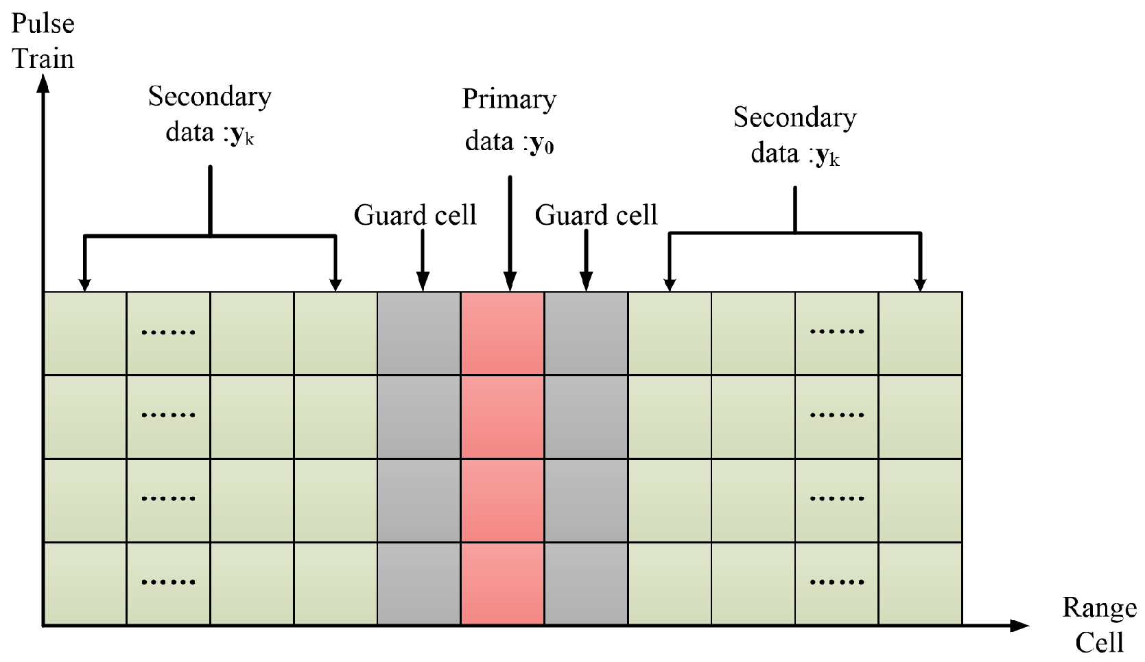
• Multiple data resources are exploited from three input channels in the network, including the primary data, secondary data, and regularization data, to raise the estimation accuracy of the clutter covariance matrix. The obtained estimation of the clutter covariance matrix is applied to the ANMF detector for target detection.
• Performance assessment is gained via both simulated and real sea clutter, illustrating the effectiveness and advancement of the estimator via CVCENet, compared with RVCENet and traditional model-based covariance matrix estimators.

The remainder of the paper is arranged as follows. A description of adaptive detection and the detection model are given in Section 2. Section 3 provides a detailed design process of the proposed network. Section 4 is devoted to the performance assessment via both simulated and real data. Section 5 concludes the paper.

2. Problem Formulation

In this section, we introduce the detection model and explain the importance of covariance matrix estimation.

A train of echo data is received from a radar system containing potential targets and environmental clutter. We take sea exploration, for example, shown in Figure 1. After pulse compression, the received echo data can be shown in Figure 2, with N pulses being in a coherent processing interval. ${\mathbf{y}}_0$ is an N-dimensional vector containing the potential target in the cell under test (CUT), named the primary data. Separated from ${\mathbf{y}}_0$ by guard cells, ${\mathbf{y}}_k,k=1,\cdots ,K$ is the N-dimensional signal-free vector called the secondary data. There is only clutter or noise in ${\mathbf{y}}_k,k=1,\cdots ,K$, which is used for clutter covariance matrix estimation, with K being the number of range cells ($K\ge N$). The detection problem can be formulated according to the following binary hypothesis test [34]

$$\left\{\begin{array}{cccc}\hfill {\mathrm{H}}_0:& {\mathbf{y}}_0={\mathbf{c}}_0,\hfill & {\mathbf{y}}_k={\mathbf{c}}_k,\hfill & k=1,\cdots ,K\hfill \\ \hfill {\mathrm{H}}_1:& {\mathbf{y}}_0=a\mathbf{s}+{\mathbf{c}}_0,\hfill & {\mathbf{y}}_k={\mathbf{c}}_k,\hfill & k=1,\cdots ,K\hfill \end{array},\right.$$

(1)

where $\mathbf{s}=\frac{1}{\sqrt{N}}{\left[1,exp\left(j2\pi f_d\right),\cdots exp\left(j2\pi \left(N-1\right)f_d\right)\right]}^T$ is the signal steering vector. $f_d$ is the normalized Doppler frequency, space frequency, or space–time frequency, depending on the type of radar system. a denotes the amplitude, which is accounted for both the target and the channel effects. ${\mathbf{c}}_k\in {\mathbb{C}}^{N\times 1},k=0,1,\cdots K$ denotes the N-dimensional clutter data.

A detector aims to detect a target under an unknown environment, which is designed to maximize the probability of detection (PD) under constant false alarm probability (CFAR). There are many detectors fit for various scenarios and conditions [35], which can be generally formulated as

$$f\left({\mathbf{y}}_0,\mathbf{Y},\mathbf{s}\right)\underset{{\mathrm{H}}_0}{\stackrel{{\mathrm{H}}_1}{\gtrless }}\eta ,$$

(2)

where $f\left(·\right)$ denotes the mapping function, $\mathbf{Y}=\left[{\mathbf{y}}_1,{\mathbf{y}}_2,\dots {\mathbf{y}}_K\right]$ is the secondary data matrix and $\eta$ is the detection threshold determined by the false alarm probability (PFA). The compound Gaussian clutter is a common type in the real world, whose optimum radar detector is named the NMF [14], i.e.,

$$\frac{{\left|{\mathbf{s}}^H{\mathbf{R}}^{-\mathbf{1}}{\mathbf{y}}_{\mathbf{0}}\right|}^2}{\left({\mathbf{s}}^H{\mathbf{R}}^{-1}\mathbf{s}\right)\left({{\mathbf{y}}_0}^H{\mathbf{R}}^{-1}{\mathbf{y}}_0\right)}\underset{{\mathrm{H}}_0}{\stackrel{{\mathrm{H}}_1}{\gtrless }}{\eta }_{\mathrm{NMF}},$$

(3)

where $\mathbf{R}$ is the true clutter covariance matrix and ${\eta }_{\mathrm{NMF}}$ is the threshold of NMF. In practice, $\mathbf{R}$ is usually unknown so that an estimation of the clutter covariance matrix $\widehat{\mathbf{R}}$ is necessary to take place $\mathbf{R}$ in (3), gaining the ANMF detector as [14],

$$\frac{{\left|{\mathbf{s}}^H{\widehat{\mathbf{R}}}^{-\mathbf{1}}{\mathbf{y}}_{\mathbf{0}}\right|}^2}{\left({\mathbf{s}}^H{\widehat{\mathbf{R}}}^{-1}\mathbf{s}\right)\left({{\mathbf{y}}_0}^H{\widehat{\mathbf{R}}}^{-1}{\mathbf{y}}_0\right)}\underset{{\mathrm{H}}_0}{\stackrel{{\mathrm{H}}_1}{\gtrless }}{\eta }_{\mathrm{ANMF}},$$

(4)

where $\widehat{\mathbf{R}}$ denotes the estimated clutter covariance matrix, and ${\eta }_{\mathrm{ANMF}}$ is the threshold of ANMF. Therefore, the estimation quality of the clutter covariance matrix is crucial to adaptive detection.

3. Covariance Matrix Estimation Network

This section gives the designing process of covariance matrix estimation based on CV-CNN. First, we introduce a classical covariance matrix estimation mathematical model, i.e., the general linear model. Next, we construct our proposed CVCENet. Then, we give the training process of the CVCENet.

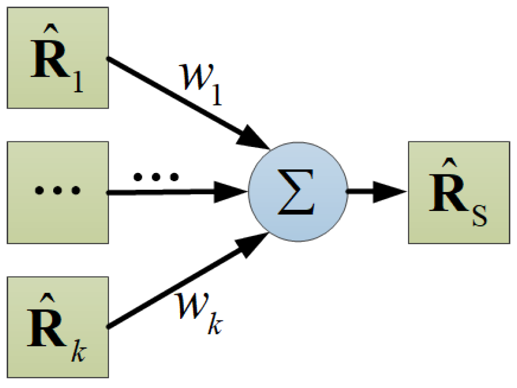
3.1. Linear Covariance Matrix Estimator

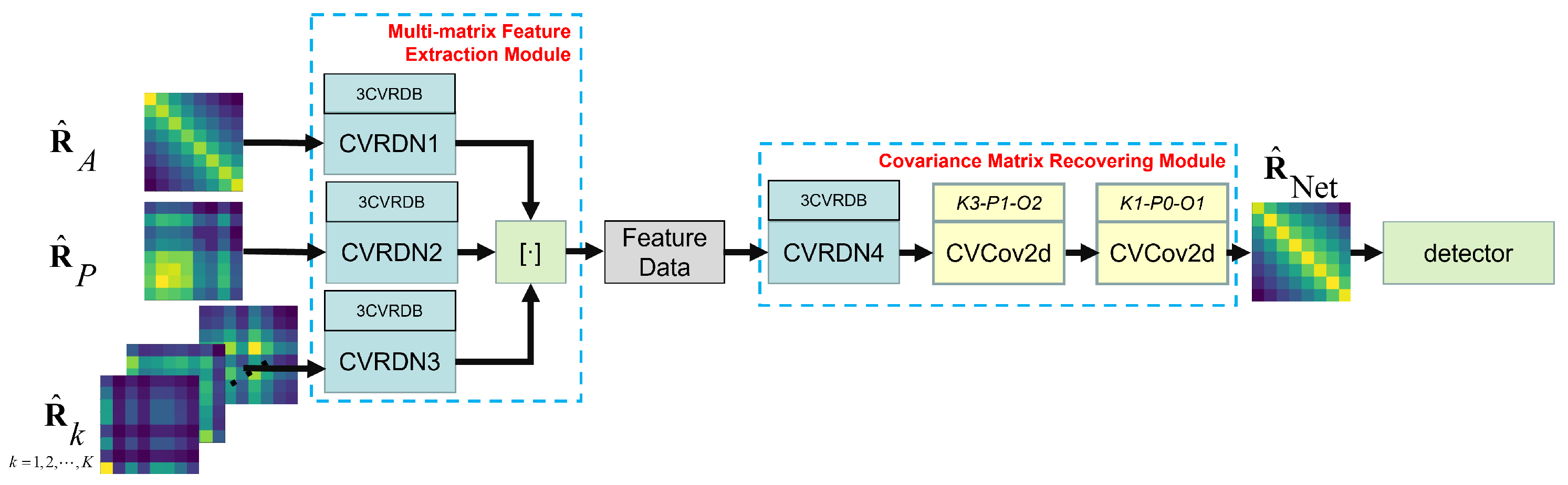
The general linear covariance matrix estimation model is formulated as [18]

$$\widehat{\mathbf{R}}=\alpha {\widehat{\mathbf{R}}}_A+(1-\alpha ){\widehat{\mathbf{R}}}_S,$$

(5)

where $\alpha$ is the linear weighting factor. ${\widehat{\mathbf{R}}}_A$ is called the estimation of the regularization covariance matrix, which can be obtained via prior information of a covariance matrix in the CUT, sometimes ${\widehat{\mathbf{R}}}_A$ can be set to be a unit matrix. ${\widehat{\mathbf{R}}}_S$ is called the estimation of a secondary covariance matrix, which can be obtained via secondary data and shown in the form of SCM, NSCM, AML, and so on. Precisely, ${\widehat{\mathbf{R}}}_S$ is a linear combination of secondary covariance matrix in different range bins, i.e.,

$${\widehat{\mathbf{R}}}_S={\Sigma }_{k=1}^{k=K}{w}_k{\widehat{\mathbf{R}}}_k,$$

(6)

where ${\widehat{\mathbf{R}}}_k,k=1,\cdots ,K$ denotes the estimated covariance matrix in different range bins, $w_k$ is the weighting factor, being constant for most covariance matrix estimators. The structure diagram of ${\widehat{\mathbf{R}}}_S$ is given in Figure 3, and three typical estimators of ${\widehat{\mathbf{R}}}_S$ are shown in

Table 1. Form of typical estimators of ${\widehat{\mathbf{R}}}_S$.

Estimator	${\mathit{w}}_{\mathit{k}}$	$\widehat{\mathbf{R}}$${}_{\mathit{k}}$
SCM [5]	$\frac{1}{K}$	${\mathbf{y}}_k{\mathbf{y}}_k^H$
NSCM [12]	$\frac{N}{K}$	$\frac{{\mathbf{y}}_k{\mathbf{y}}_k^H}{{\mathbf{y}}_k^H{\mathbf{y}}_k}$
AML [13]	$\frac{N}{K}$	$\frac{{\mathbf{y}}_k{\mathbf{y}}_k^H}{{\mathbf{y}}_k^H{\widehat{\mathbf{R}}}_{\left(i\right)}^{-1}{\mathbf{y}}_k}$

, where ${\widehat{\mathbf{R}}}_{\left(i\right)}^{-1}$ is the inverse of covariance matrix estimation of the ith iteration, especially for ${\widehat{\mathbf{R}}}_{\left(0\right)}^{-1}=\mathbf{I}$.

3.2. CVCENet

Considering it is hard to model the covariance matrix in the real world as a specific mathematical model, we depend on a data-driven method to estimate the covariance matrix. As shown in Figure 3, the structure of ${\widehat{\mathbf{R}}}_S$ is similar to a single layer fully connected network without an activation function, driving us to design a general covariance matrix estimation network, given as

$${\widehat{\mathbf{R}}}_{\mathrm{Net}}=f({\widehat{\mathbf{R}}}_A,{\widehat{\mathbf{R}}}_P,{\widehat{\mathbf{R}}}_k|\Theta ),$$

(7)

where ${\widehat{\mathbf{R}}}_P$ denotes the primary covariance matrix, i.e., the covariance matrix of clutter data in the CUT. $\Theta$ is the weighting factor vector of the net, which can be obtained via gradient descent optimization algorithm [36,37].

The CVCENet is generally composed of a multi-matrix feature extraction module and a covariance matrix recovering module, whose framework is shown in Figure 4, where $\left[·\right]$ denotes the concat function. The input of CVCENet comes from ${\widehat{\mathbf{R}}}_A$, ${\widehat{\mathbf{R}}}_P$, and ${\widehat{\mathbf{R}}}_k,k=1,\cdots ,K$, and the output is ${\widehat{\mathbf{R}}}_{\mathrm{Net}}$. We use simulated compound Gaussian clutter data and NSCM to generate ${\widehat{\mathbf{R}}}_P$ and ${\widehat{\mathbf{R}}}_k,k=1,\cdots ,K$, while ${\widehat{\mathbf{R}}}_A$ is obtained via historical data [38] or a unit matrix, which will be specifically stated in the training process. Substituting the gained ${\widehat{\mathbf{R}}}_{\mathrm{Net}}$ into a suitable detector, with ANMF being applied in the paper, we obtain the final detection results.

The multi-matrix feature extraction module is composed of three CV residual dense networks (CVRDNs). Each CVRDN contains three CV residual dense blocks (CVRDBs), labeled at the top of the CVRDN as its main block. As for the covariance matrix recovering module, it is constructed by a CVRDN and two complex-valued convolutional layers of two-dimension, i.e., CVCov2d, with different parameter settings labeled at the top. For example, “$K3-P1-O2$” denotes the parameter setting of the first CVCov2d, i.e., kernel size 3 × 3, padding 1, output channel number 2. All the parameter settings aim to make the dimensions of output identical to the input, which can be referred to in [39]. In the subsequent, we will give elaborate descriptions of the CVCENet module by module.

Multi-matrix feature extraction module: It is the starting module of the CVCENet, constructed by three CVRDNs, i.e., CVRDN1, CVRDN2, and CVRDN3, corresponding to the inputs of ${\widehat{\mathbf{R}}}_A$, ${\widehat{\mathbf{R}}}_P$, and ${\widehat{\mathbf{R}}}_k,$$k=1,\cdots ,K$, respectively. Making a concat to the three CVRDNs yields the output of the module, i.e., feature data of the covariance matrix to be estimated. For each CVRDN, three CVRDBs are contained as the main block. Actually, RDN and RDB are usually adopted to obtain a super-resolution image. CVRDN and CVRDB are the extending complex-valued operations of RDN and RDB, respectively, aiming to deal with the estimation of the covariance matrix, which seems to be a complex-valued image. This is why we chose CVRDN and CVRDB as the basic blocks of the module, whose structures are given in Figure 5 and Figure 6, respectively. The double line arrows in Figure 5 and Figure 6 stand for the residual connect [40], which is an effective architecture to prevent the disappearance of gradients during the training process and has been widely used for neural network construction, marked in different colors merely for clarification. Moreover, the CVCov2d provides a similar calculation rule as a real-valued convolution layer, except for its complex-valued operations. The split complex rectified linear units, i.e., CRelu, is a calculation unit that is ruled as [30],

$$\mathbf{CRelu}\left(\mathbf{Z}\right)=\max \left(0,\Re \left(\mathbf{Z}\right)\right)+j\max \left(0,\Im \left(\mathbf{Z}\right)\right),$$

(8)

where $\Re \left(\mathbf{Z}\right)$ and $\Im \left(\mathbf{Z}\right)$ denote the real and imaginary parts of $\mathbf{Z}$, respectively.

Covariance Matrix Recovering Module: With the feature data of covariance matrix to be estimated, the data are fed to the covariance matrix recovering module to obtain ${\widehat{\mathbf{R}}}_{\mathrm{Net}}$. The module consists of a CVRDN, i.e., CVRDN4, and two CVCov2ds with different parameter settings, aiming to obtain the ${\widehat{\mathbf{R}}}_{\mathrm{Net}}$ under desirable dimensions. The details of CVRDN and CVCov2d have just been discussed in the multi-matrix feature extraction module.

To verify the advancement of the CV network, we also construct an RV network as a natural competitor for comparison, i.e., RVCENet, with the same framework as that of CVCENet. In RVCENet, all the input data are separated as real and imaginary parts, stream into the network simultaneously with real-valued calculations, obtaining the real and imaginary parts of ${\widehat{\mathbf{R}}}_{\mathrm{Net}}$. We make a concat to the real and imaginary parts and recover the ${\widehat{\mathbf{R}}}_{\mathrm{Net}}$ in the end.

3.3. Training Process

Because the true covariance matrix of measured data is hard to obtain, we use the simulated data to produce the training data set (TDS) as the ground truth covariance matrix and train our CVCENet.

3.3.1. Simulated Data Configuration

In this paper, the compound Gaussian clutter is adopted as the simulated clutter, whose probability density function (PDF) can be formulated as [41]

$$p\left({\mathbf{c}}_k\right)=\frac{exp\left(\frac{{\mathbf{c}}_k^H{\mathbf{R}}^{-1}{\mathbf{c}}_k}{{\tau }_k}\right)}{{\pi }^N{\tau }_k^N\left|\mathbf{R}\right|},k=0,1,2,\cdots ,K,$$

(9)

where $p(·)$ denotes the PDF function, ${\tau }_k,k=0,\cdots ,K$ is a set of positive random numbers, which is called the texture component and determined by the local scattering power. Moreover, ${\tau }_k,k=0,\cdots ,K$ can be modeled to follow the Gamma [42], inverse Gamma [34,43], inverse Gaussian [44] distribution, and so on. In [1,34,43], it is suggested that sea clutter can be depicted as compound Gaussian clutter with texture component ${\tau }_k$ following the inverse Gamma distribution, i.e.,

$$p\left({\tau }_k\right)=\frac{1}{{\mu }^{\lambda }\Gamma \left(\lambda \right)}{\tau }^{-(\lambda +1)}exp\left(-\frac{1}{\mu {\tau }_k}\right),$$

(10)

where $\lambda$ denotes the shape parameter, $\mu$ denotes the scale parameter, with both $\lambda$ and $\mu$ being positive.

The clutter covariance matrix can be modeled as

$$\mathbf{R}={\sigma }_c^2\mathbf{M}+{\sigma }_n^2\mathbf{I},$$

(11)

where ${\sigma }_{\mathrm{c}}^2$ is the power of the clutter and ${\sigma }_{\mathrm{n}}^2$ is the power of the thermal noise. $\mathbf{M}$ is the structure of the clutter covariance matrix, with the form [45]

$$\mathbf{M}\left(i,j\right)={\rho }^{\left|i-j\right|}exp\left(f_c\left(i-j\right)\right),i,j=1,\cdots ,N,$$

(12)

where $\rho \in (0,1)$ is the one-lag correlation coefficient, $f_c$ is the normalized Doppler frequency of clutter. $f_c$ is usually caused in two ways: one is the motion of the detection platform, such as clutter of aircraft detection for ground targets, and the other is the internal motion of clutter, such as the moving sea wave. According to (1), (11) and (12), we can define the clutter-to-noise ratio (CNR) and the signal-to-clutter-noise ratio (SCNR) as [21]

$$\mathrm{CNR}=\frac{{\sigma }_{\mathrm{c}}^2}{{\sigma }_{\mathrm{n}}^2},$$

(13)

$$\mathrm{SCNR}={\left|a\right|}^2{\mathbf{s}}^H{\mathbf{R}}^{-1}\mathbf{s}.$$

(14)

3.3.2. Training Process Description

During the training process, we use simulated clutter to generate $\mathbf{R}$, called the ground truth covariance matrix, with $\rho \sim \mathrm{U}(0.8,0.95)$, $f_c\sim \mathrm{U}(-0.2,0.2)$, $\mathrm{CNR}\sim \mathrm{U}(20,50)\mathrm{dB}$, where $\mathrm{U}\left(·,·\right)$ denotes the uniform distribution. ${\tau }_k$ follows the inverse Gamma distribution with $\lambda \sim \mathrm{U}(1.5,5)$, $\mu \sim \mathrm{U}(0.5,1.5)$. To obtain ${\widehat{\mathbf{R}}}_{\mathrm{Net}}$, we train 200 epochs. For each epoch, we produce ${10}^4$ sets of data, including $\mathbf{R}$, ${\widehat{\mathbf{R}}}_A$, ${\widehat{\mathbf{R}}}_P$, ${\widehat{\mathbf{R}}}_k,k=1,\cdots ,K$. The batch size is fixed at 16. For all convolutional layers, the learning rate is initialized at ${10}^{-4}$ and halves for every 50 epochs. Please note that ${\widehat{\mathbf{R}}}_A$ has $50\%$ chance to be set as ${\widehat{\mathbf{R}}}_A=\mathbf{I}$, and another $50\%$ chance to be set as a dot product between a prior covariance matrix based on the ground truth matrix $\mathbf{R}$ and a perturbed matrix [18], i.e.,

$${\widehat{\mathbf{R}}}_A=\mathbf{R}\odot \mathbf{t}{\mathbf{t}}^T,$$

(15)

where ${(·)}^T$ denotes the transpose operator, ⊙ denotes the Hadamard matrix product, and $\mathbf{t}$ is a vector of independent identically distributed (IID) Gaussian random variables with mean 1, variance ${\sigma }_t^2\sim \mathrm{U}(0.01,0.9)$.

For performance assessment of the CVCENet, the mean squared error loss (MSELoss) function is adopted to evaluate the discrepancy between the predicted covariance matrix and the ground truth covariance matrix, which is also applied in traditional linear covariance matrix estimation model [18,21], given as,

$$L={∥{\widehat{\mathbf{R}}}_{\mathrm{Net}}-\mathbf{R}∥}_2^2,$$

(16)

where ${\parallel ·\parallel }_2^2$ denotes the square of 2-norm. During each epoch, the training data are randomly generated with the parameter vector $\Theta$ updated by gradient descent optimization algorithms [46]. To interpret the training process more clearly, we sum up the details of the hyperparameters and training strategy, shown in

Table 2. List of hyperparameters.

Hyperparameter	Value
batch size	16
number of samples of each epoch	10,000
number of epoch	200
learning rate	0.001
learning rate decay	0.5 for every 50 epochs
optimizer	Adam

and

Table 3. Training strategy.

CVCENet
for epoch = 1:200 do
(1) Set $\rho \sim \mathrm{U}(0.8,0.95)$   (2) Set $f_c\sim \mathrm{U}(-0.2,0.2)$   (3) Set $\mathrm{CNR}\sim \mathrm{U}(20,50)\mathrm{dB}$   (4) Set $\lambda \sim \mathrm{U}(1.5,5)$   (5) Set $\mu \sim \mathrm{U}(0.5,1.5)$   (6) Generate $\mathbf{R}$ according to Equations (11)–(13)     for t = 1:10,000 do      (1) Given $\lambda ,\mu$, generate ${\tau }_k,k=0,1,\cdots ,K$, according to Equation (10)      (2) Given $\mathbf{R},{\tau }_k,k=0,1,\cdots ,K$, generate ${\mathbf{c}}_k,k=0,1,\cdots ,K$ according to Equation (9)      (3) Generate ${\widehat{\mathbf{R}}}_P$ and ${\widehat{\mathbf{R}}}_k,k=1,\cdots ,K$ via ${\mathbf{c}}_k,k=0,\cdots ,K$ and NSCM      (4) Set a temporary random variable $tmp\sim \mathrm{U}(0,1)$        if $tmp<0.5$            Set ${\widehat{\mathbf{R}}}_A=\mathbf{I}$        else         (1) Set ${\sigma }_t^2\sim \mathrm{U}(0.01,0.9)$ in Equation (15)         (2) Generate $\mathbf{t}$ and obtain ${\widehat{\mathbf{R}}}_A$ according to Equation (15)        end if       (5) Put the generated ${\widehat{\mathbf{R}}}_A,{\widehat{\mathbf{R}}}_P,{\widehat{\mathbf{R}}}_k,k=1,\cdots ,K$ into the three input channels and obtain the output ${\widehat{\mathbf{R}}}_{\mathrm{Net}}$      (6) Calculate L according to Equation (16)      (7) Update $\Theta$ via gradient descent optimization algorithms      end for
end for

, respectively.

4. Experimental Results and Analysis

In this section, we use the simulated clutter and the real sea clutter from IPIX radar to test the efficiency of our proposed CVCENet. We begin with a discussion about the measured data. The training and detection performances of CVCENet are then analyzed.

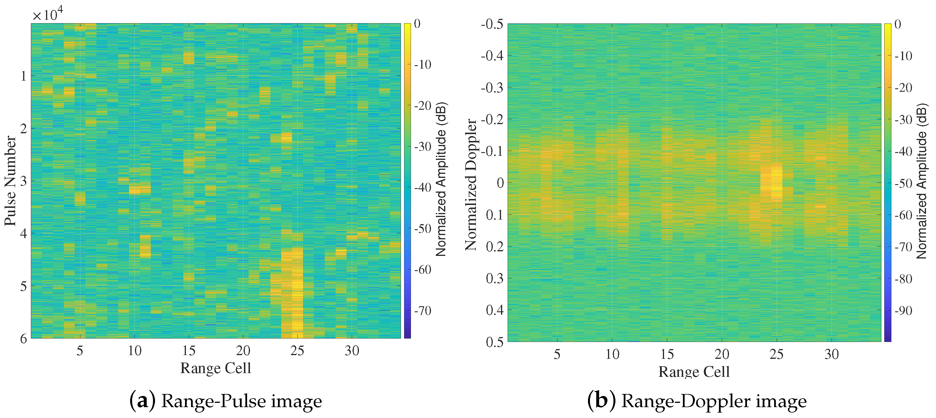
4.1. Measured Data Configuration

In the testing phase, both simulated and measured data are used for the performance assessment of our proposed network. The generation method of simulated data for testing is the same as that in the training process. The adopted measured data are collected by the IPIX radar system [47,48]. We use the data from the 19980223_170435_ANTSTEP.CDF data file, which consists of 60,000 coherent pulse trains and 34 range cells, with the parameter setting shown in

Table 4. The system parameters of the IPIX radar system.

19980223_170435_ANTSTEP.CDF
Date and time (UTC)	23 February 1998 17:04:35
RF frequency	9.39 GHz
Pulse length	100 ns
Pulse repetition frequency	1000 Hz
Radar azimuth angle	${346.75}^{\circ }$
Range	3500–4000 m
Range resolution	15 m
Radar beamwidth	${0.9}^{\circ }$

. The Range-Pulse image and Range-Doppler image of this dataset are shown in Figure 7a,b, respectively.

As is shown in Figure 7, there is clutter with relatively strong power in the 25th range cell, which has a wide band of normalized Doppler frequency (between about −0.1 and 0.1). Please note that the detection performance will decline when the normalized Doppler frequency of target approaches is close to that of clutter.

4.2. Experimental Results

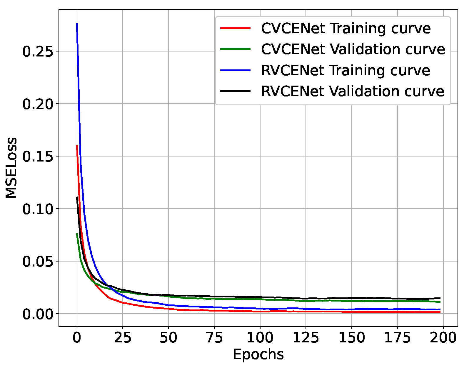
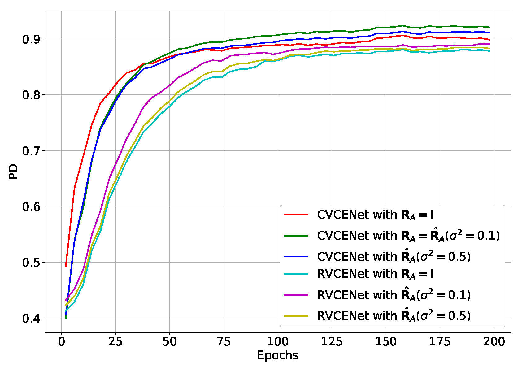
4.2.1. Training Results

The mean squared error loss (MSELoss) curves of training and validation at each epoch are shown in Figure 8. It is observed that the training loss decreases as the number of epochs increases, and a similar trend can be found in the curve of validation loss despite a small performance difference between training and validation sets. Moreover, they all converge at about 100 epochs. The results in Figure 8 illustrate that both the CVCENet and the RVCENet have been trained and are ready for the testing phase. The source code for both networks is given at: https://github.com/JShangS/CVCENet.git (accessed on 12 November 2023).

To analyze the performance of our proposed covariance matrix estimation network, we apply CVCENet to the ANMF to compare the detection results with other estimators, i.e., $\widehat{\mathbf{R}}$ is replaced by the CVCENet, RVCENet, NSCM, and SFPE. To obtain the decision thresholds for a given PFA = ${10}^{-3}$, we use the standard Monte Carlo technique based on 100/PFA independent trials. We also use ${10}^4$ Monte Carlo trials to calculate the PD of the ANMF detectors via the four covariance matrix estimators.

Figure 9 further shows the network performance of the training phase. With the increase of training epochs, the PD of CVCENet increases faster than RVCENet and all the PDs tend to converge to stable values at about 100 epochs, which coincides with the results in Figure 8. The results in Figure 8 and Figure 9 show that the CVCENet has lower estimation loss and faster convergence rate in the training phase than that of the RVCENet, suggesting that the CVCENet may have better detection performance than the RVCENet. Next, we use the trained CVCENet and RVCENet to do further analyses of detection performance.

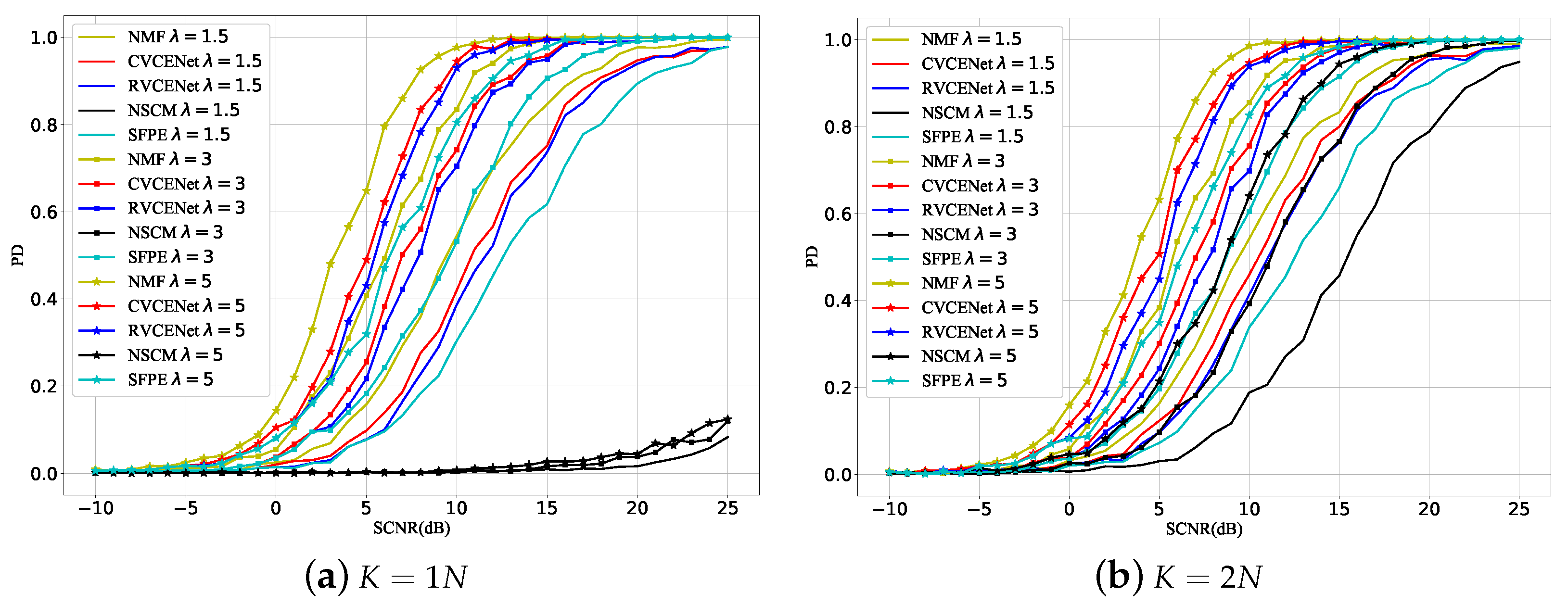
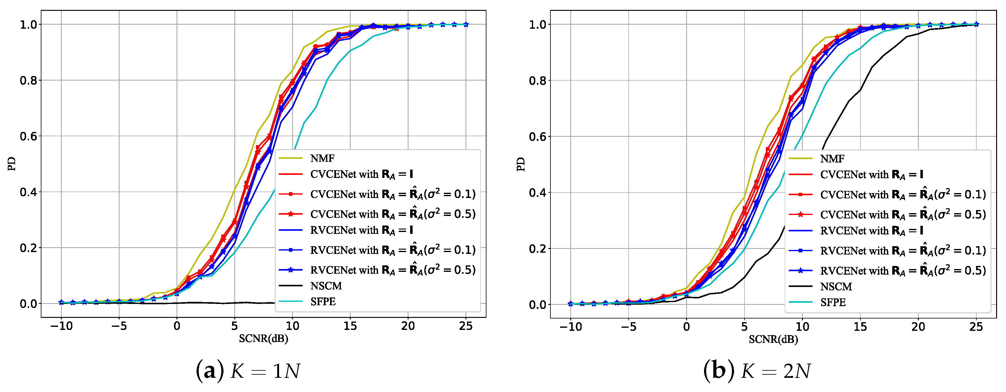
4.2.2. Detection Results with Simulated Data

We compare the detection performance of ANMF via different covariance matrix estimators under different shape parameters. The results are shown in Figure 10. The applied parameters in this experiment are set to $\lambda =1.5$, 3, 5, $\mu =1$ and ${\mathbf{R}}_{\mathrm{A}}=\mathbf{I}$. The detection results in Figure 10 show that the detection performance of all the detectors improves as $\lambda$ increases because the non-Gaussian property of clutter decreases [34]. The ANMF with CVCENet has the best detection performance under cases of different $\lambda$. The ANMF with RVCENet has better performance than SFPE and NSCM, while there is a gap with the CVCENet. Thanks to the regularization item, the CVCENet, RVCENet, and SFPE can handle a small number of secondary data issues, i.e., $K=1N$, while NSCM shows to be ineffective.

To study the effect of regularization, we further test the performance of the estimators under different regular terms ${\mathbf{R}}_A$, with the results shown in Figure 11, where the smaller ${\sigma }^2$ means a more precise prior covariance matrix. One can find that the CVCENet with ${\mathbf{R}}_A={\widehat{\mathbf{R}}}_A({\sigma }^2=0.1)$ has the best detection property. The RVCENet can also make good use of the prior covariance matrix, but the PD is lower than the CVCENet with the same regular terms. The SFPE can only use $\mathbf{I}$ as the regularization, so it cannot be further improved via the prior covariance matrix. In addition, the NSCM can only exploit the secondary data to estimate the clutter covariance matrix, which makes it hard to further improve estimation performance, especially in the case of a small number of secondary data.

The effect of target velocity or target normalized Doppler frequency on PD is shown in Figure 12. The SCNR is set to 15 dB, and the sampling interval of the target normalized Doppler frequency is 0.05. The trend of PD in Figure 12 shows that the performance of all the detectors increases gradually as the target normalized Doppler frequency moves away from the center of the clutter normalized Doppler frequency. The CVCENet has a relatively tighter notch than the other estimators. When $f_d<0.1$, it is close to the theoretically optimal detection results, i.e., the result of NMF (solid yellow line in Figure 12). Furthermore, the proposed estimator can make efficient use of the prior information ${\widehat{\mathbf{R}}}_A$, when prior information becomes bad, i.e., ${\sigma }^2=0.5$, the performance of the proposed estimator has only slightly decreased.

4.2.3. Detection Results with IPIX Radar Data

With the visual representation of the data shown in Figure 7, we choose the 25th range cell as the CUT and adopt $K=1N,2N$ surrounding cells as secondary data, i.e., the range cells from 16 to 23 as well as 26 to 33. We apply all the available temporal samples under $N=8$ (the red rectangular box in Figure 13) for statistical tests. For each test, we add targets with different SCNR and $f_d$ in CUT. According to [38,49], we adopt the previous 100 pulses in the 25th range cell data as the historical data, aiming to estimate the prior covariance matrix as the regularization covariance matrix ${\widehat{\mathbf{R}}}_A$. The estimation process is shown in Figure 13. We slide the yellow rectangular box to calculate the ith covariance matrix ${\widehat{\mathbf{R}}}_A^i$, namely

$${\widehat{\mathbf{R}}}_A^i={\mathbf{y}}_{\mathrm{CUT}}^i\mathbf{y}{{}_{\mathrm{CUT}}^i}^H$$

(17)

where ${\mathbf{y}}_{\mathrm{CUT}}^i$ is the ith sliding vector in the CUT. Then, we average the sum of ${\widehat{\mathbf{R}}}_A^i,i=1\cdots N_t$, to obtain the regularization covariance matrix ${\widehat{\mathbf{R}}}_A$

$${\widehat{\mathbf{R}}}_A=\frac{1}{N_{\mathrm{t}}}\sum _{i=1}^{N_{\mathrm{t}}-1}{\widehat{\mathbf{R}}}_A^i$$

(18)

where $N_{\mathrm{t}}=100$. After the above pretreatment, we test the performance of the proposed network as follows.

Figure 14 shows the detection performance under different SCNR. It can be found that ANMF with the CVCENet has a clear advantage over other estimators, particularly under low SCNR. ANMF detector with RVCENet performs better than the SFPE and NSCM while worse than the CVCENet. When using simulated data, however, the discrepancy between CVCENet and RVCENet is not so clear.

Figure 15 depicts the influence of clutter Doppler frequency on target detection when using different covariance estimators. In this figure, it is observed that when the clutter has a wide band near the clutter Doppler frequency, all the detectors have bad detection results. The detection performance of the CVCENet rises fastest when the target Doppler frequency moves away from the clutter region. Furthermore, all the network covariance estimators have better performance than the traditional estimators involved in the comparison.

For intuitive comparison, we summarize the properties of our proposed network estimators and traditional model-based estimators, shown in

Table 5. Summary of various clutter covariance matrix estimators.

Method	Convergence Property	Data Resource		Detection Performance
		Primary Data	Regularization Data	Insufficient Secondary Data	PD Rank
CVCENet	Faster convergence than RVCENet	applied	applied	effective	1
RVCENet	Slower convergence than CVCENet	applied	applied	effective	2
NSCM [12]	Closed solution without convergence	not applied	not applied	noneffective	4
SFPE [15]	Closed solution without convergence	not applied	only unit matrix is applied	effective	3

. Besides the secondary data, our proposed CVCENet exploits the primary and regularization data for clutter covariance matrix estimation with faster convergence than the RVCENet. The detector with the CVCENet shows the highest PD and is also efficient under insufficient secondary data.

In addition, we will try to explain why the CVCENet can obtain the best results. Compared with RVCENet, the main difference between the two networks is the multiplication rule. As Hirose [32] suggested, complex multiplication could reduce the ineffective degree of freedom and enforce signal transformations according to the physical characteristics of the data. Therefore, the complex-valued calculation rule can accelerate convergence in the training phase and obtain better adaptability to data. Compared with traditional methods, the performance of estimators based on neural networks benefits from large amounts of data generated under various conditions. In fact, high-quality training data are the key to the performance of the network. We use the data generated under different models to train our network, surely exceeding the performance of the estimator obtained via only one model. In other words, our proposed network can be seen as an estimator that uses large amounts of current data and historical data to estimate the true covariance matrix, which is different from the traditional estimators that only use the current data.

5. Conclusions

In this paper, we have proposed a CV covariance matrix estimation network, named the CVCENet, to deal with radar adaptive detection under non-Gaussian clutter. An RV network with the same framework as the CVCENet is also constructed as the natural competitor, named the RVCENet. Both simulated and real sea clutter have been used to evaluate the performance of the proposed estimator based on the network. In the training process, it is illustrated that the CVCENet has a faster convergence rate than the RVCENet and reaches the stable PD earlier than the RVCENet. As for detection performance, the detector with the proposed CVCENet has better PD than traditional estimators, as well as the detector with RVCENet, under a sufficient or small number of secondary data. The follow-up work on this study may involve applying more sea clutter data to further train the network for better performance.

References

1. Conte, E.; De Maio, A. Mitigation techniques for non-Gaussian sea clutter. IEEE J. Ocean. Eng. 2004, 29, 284–302. [Google Scholar] [CrossRef]
2. Xue, J.; Xu, S.; Liu, J. Persymmetric Detection of Radar Targets in Nonhomogeneous and Non-Gaussian Sea Clutter. IEEE Trans. Geosci. Remote. Sens. 2022, 60, 1–9. [Google Scholar] [CrossRef]
3. Brennan, L.; Reed, L. Theory of Adaptive Radar. IEEE Trans. Aerosp. Electron. Syst. 1973, AES-9, 237–252. [Google Scholar] [CrossRef]
4. Ward, J. Space-time adaptive processing for airborne radar. In Proceedings of the IEE Colloquium on Space-Time Adaptive Processing, London, UK, 6 April 1998; pp. 2/1–2/6. [Google Scholar]
5. Goodman, N.R. Statistical Analysis Based on a Certain Multivariate Complex Gaussian Distribution (An Introduction). Ann. Math. Stat. 1963, 34, 152–177. [Google Scholar] [CrossRef]
6. Liu, W.; Xie, W.; Liu, J.; Wang, Y. Adaptive Double Subspace Signal Detection in Gaussian Background—Part I: Homogeneous Environments. IEEE Trans. Signal Process. 2014, 62, 2345–2357. [Google Scholar] [CrossRef]
7. Kelly, E. An Adaptive Detection Algorithm. IEEE Trans. Aerosp. Electron. Syst. 1986, AES-22, 115–127. [Google Scholar] [CrossRef]
8. Robey, F.C.; Fuhrmann, D.R.; Kelly, E.J.; Nitzberg, R. A CFAR adaptive matched filter detector. IEEE Trans. Aerosp. Electron. Syst. 1992, 28, 208–216. [Google Scholar] [CrossRef]
9. Gini, F.; Farina, A. Vector subspace detection in compound-Gaussian clutter. Part I: Survey and new results. IEEE Trans. Aerosp. Electron. Syst. 2002, 38, 1295–1311. [Google Scholar] [CrossRef]
10. Gini, F.; Farina, A.; Montanari, M. Vector subspace detection in compound-Gaussian clutter, part II: Performance analysis. IEEE Trans. Aerosp. Electron. Syst. 2002, 38, 1312–1323. [Google Scholar] [CrossRef]
11. Pascal, F.; Chitour, Y.; Ovarlez, J.P.; Forster, P.; Larzabal, P. Covariance Structure Maximum-Likelihood Estimates in Compound Gaussian Noise: Existence and Algorithm Analysis. IEEE Trans. Signal Process. 2007, 56, 34–48. [Google Scholar] [CrossRef]
12. Gini, F.; Michels, J.H. Performance analysis of two covariance matrix estimators in compound-Gaussian clutter. IEE Proc.—Radar Sonar Navig. 2002, 146, 133–140. [Google Scholar] [CrossRef]
13. Gini, F.; Greco, M. Covariance matrix estimation for CFAR detection in correlated heavy tailed clutter. Signal Process. 2002, 82, 1847–1859. [Google Scholar] [CrossRef]
14. Conte, E.; Lops, M.; Ricci, G. Adaptive detection schemes in compound-Gaussian clutter. IEEE Trans. Aerosp. Electron. Syst. 1998, 34, 1058–1069. [Google Scholar] [CrossRef]
15. Chen, Y.; Wiesel, A.; Hero Alfred, O.I. Robust Shrinkage Estimation of High-Dimensional Covariance Matrices. IEEE Trans. Signal Process. 2011, 59, 4097–4107. [Google Scholar] [CrossRef]
16. Pascal, F.; Chitour, Y.; Quek, Y. Generalized Robust Shrinkage Estimator and Its Application to STAP Detection Problem. IEEE Trans. Signal Process. 2013, 62, 5640–5651. [Google Scholar] [CrossRef]
17. Kammoun, A.; Couillet, R.; Pascal, F.; Alouini, M.S. Optimal Design of the Adaptive Normalized Matched Filter Detector using Regularized Tyler Estimators. IEEE Trans. Aerosp. Electron. Syst. 2018, 54, 755–769. [Google Scholar] [CrossRef]
18. Stoica, P.; Li, J.; Zhu, X.; Guerci, J.R. On Using a priori Knowledge in Space-Time Adaptive Processing. IEEE Trans. Signal Process. 2008, 56, 2598–2602. [Google Scholar] [CrossRef]
19. Riedl, M.; Potter, L.C. Multimodel Shrinkage for Knowledge-Aided Space-Time Adaptive Processing. IEEE Trans. Aerosp. Electron. Syst. 2018, 54, 2601–2610. [Google Scholar] [CrossRef]
20. Zhu, X.; Li, J.; Stoica, P. Knowledge-Aided Space-Time Adaptive Processing. IEEE Trans. Aerosp. Electron. Syst. 2011, 47, 1325–1336. [Google Scholar] [CrossRef]
21. Shang, Z.; Huo, K.; Liu, W.; Sun, Y.; Wang, Y. Knowledge-aided covariance estimate via geometric mean for adaptive detection. Digit. Signal Process. 2020, 97, 102616. [Google Scholar] [CrossRef]
22. Krichen, M. Convolutional Neural Networks: A Survey. Computers 2023, 12, 151. [Google Scholar] [CrossRef]
23. Alahmari, F.; Naim, A.; Alqahtani, H. E-Learning Modeling Technique and Convolution Neural Networks in Online Education; River Publishers: Aalborg, Denmark, 2022; pp. 261–296. [Google Scholar] [CrossRef]
24. Duan, K.; Chen, H.; Xie, W.; Wang, Y. Deep learning for high-resolution estimation of clutter angle-Doppler spectrum in STAP. IET Radar Sonar Navig. 2022, 16, 193–207. [Google Scholar] [CrossRef]
25. Wang, J.; Li, S. Maritime Radar Target Detection in Sea Clutter Based on CNN with Dual-Perspective Attention. IEEE Geosci. Remote Sens. Lett. 2023, 20, 1–5. [Google Scholar] [CrossRef]
26. Feintuch, S.; Permuter, H.H.; Bilik, I.; Tabrikian, J. Neural Network-Based Multitarget Detection within Correlated Heavy-Tailed Clutter. IEEE Trans. Aerosp. Electron. Syst. 2023, 59, 5684–5698. [Google Scholar] [CrossRef]
27. Jiang, W.; Haimovich, A.M.; Govoni, M.; Garner, T.; Simeone, O. Fast Data-Driven Adaptation of Radar Detection via Meta-Learning. In Proceedings of the 2021 55th Asilomar Conference on Signals, Systems, and Computers, Pacific Grove, CA, USA, 31 October–3 November 2021. [Google Scholar]
28. Pan, M.; Chen, J.; Wang, S.; Dong, Z. A Novel Approach for Marine Small Target Detection Based on Deep Learning. In Proceedings of the 2019 IEEE 4th International Conference on Signal and Image Processing (ICSIP), Wuxi, China, 19–21 July 2019. [Google Scholar]
29. Jarabo-Amores, M.-P.; David de la Mata-Moya, R.G.P.; Rosa-Zurera, M. Radar detection with the Neyman–Pearson criterion using supervised-learning-machines trained with the cross-entropy error. EURASIP J. Adv. Signal Process. 2013, 2013, 44. [Google Scholar] [CrossRef]
30. Su, N.; Chen, X.; Jian, G.; Li, Y. Deep CNN-Based Radar Detection for Real Maritime Target Under Different Sea States and Polarizations. In Proceedings of the 3rd International Conference on Cognitive Systems and Information Processing, Singapore, 27 April 2019. [Google Scholar]
31. López-Risueño, G.; Grajal, J.; Haykin, S.; Díaz-Oliver, R. Convolutional Neural Networks for Radar Detection. Lect. Notes Comput. Sci. 2002, 2415, 1150–1155. [Google Scholar]
32. Hirose, A. Complex-valued neural networks: The merits and their origins. In Proceedings of the 2009 International Joint Conference on Neural Networks, Atlanta, GA, USA, 14–19 June 2009; pp. 1237–1244. [Google Scholar] [CrossRef]
33. Fuchs, A.; Rock, J.; Toth, M.; Meissner, P.; Pernkopf, F. Complex-valued Convolutional Neural Networks for Enhanced Radar Signal Denoising and Interference Mitigation. In Proceedings of the 2021 IEEE Radar Conference (RadarConf21), Atlanta, GA, USA, 7–14 May 2021; pp. 1–6. [Google Scholar] [CrossRef]
34. Shang, Z.; Li, X.; Liu, Y.; Wang, Y.; Liu, W. GLRT detector based on knowledge aided covariance estimation in compound Gaussian environment. Signal Process. 2019, 155, 377–383. [Google Scholar] [CrossRef]
35. Liu, W.; Liu, J.; Hao, C.; Gao, Y.; Wang, Y. Multichannel adaptive signal detection: Basic theory and literature review. Sci. China Inf. Sci. 2022, 65, 1–40. [Google Scholar] [CrossRef]
36. Bassey, J.; Qian, L.; Li, X. A Survey of Complex-Valued Neural Networks. arXiv 2021, arXiv:2101.12249. [Google Scholar]
37. Mu, H.; Zhang, Y.; Jiang, Y.; Ding, C. CV-GMTINet: GMTI Using a Deep Complex-Valued Convolutional Neural Network for Multichannel SAR-GMTI System. IEEE Trans. Geosci. Remote Sens. 2021, 60, 1–15. [Google Scholar] [CrossRef]
38. Bidon, S.; Besson, O.; Tourneret, J.Y. Knowledge-Aided STAP in Heterogeneous Clutter using a Hierarchical Bayesian Algorithm. IEEE Trans. Aerosp. Electron. Syst. 2011, 47, 1863–1879. [Google Scholar] [CrossRef]
39. van der, M.; Kilian, Q.; Weinberger, G.H.L.P. Convolutional Networks with Dense Connectivity. IEEE Trans. Pattern Anal. Mach. Intell. 2019, 44, 8704–8716. [Google Scholar]
40. He, K.; Zhang, X.; Ren, S.; Sun, J. Deep Residual Learning for Image Recognition. In Proceedings of the 2016 IEEE Conference on Computer Vision and Pattern Recognition (CVPR), Las Vegas, NV, USA, 26 June–1 July 2016; pp. 770–778. [Google Scholar] [CrossRef]
41. Kang, N.; Shang, Z.; Du, Q. Knowledge-Aided Structured Covariance Matrix Estimator Applied for Radar Sensor Signal Detection. Sensors 2019, 19, 664. [Google Scholar] [CrossRef] [PubMed]
42. Gini, F. Sub-optimum coherent radar detection in a mixture of K-distributed and Gaussian clutter. IEE Proc.—Radar Sonar Navig. 2002, 144, 39–48. [Google Scholar] [CrossRef]
43. Xue, J.; Xu, S.W.; Shui, P. Near-optimum coherent CFAR detection of radar targets in compound-Gaussian clutter with inverse Gaussian texture. Signal Process. 2020, 166, 107236. [Google Scholar] [CrossRef]
44. Ollila, E.; Tyler, D.E.; Koivunen, V.; Poor, H.V. Compound-Gaussian Clutter Modeling with an Inverse Gaussian Texture Distribution. IEEE Signal Process. Lett. 2012, 19, 876–879. [Google Scholar] [CrossRef]
45. Shang, Z.; Huo, K.; Liu, W.; Wang, Y.; Li, X. Interference Environment Model Recognition for Robust Adaptive Detection. IEEE Trans. Aerosp. Electron. Syst. 2020, 56, 2850–2861. [Google Scholar] [CrossRef]
46. Ruder, S. An overview of gradient descent optimization algorithms. arXiv 2016, arXiv:1609.04747. [Google Scholar]
47. Conte, E.; Maio, A.D.; Galdi, C. Statistical analysis of real clutter at different range resolutions. IEEE Trans. Aerosp. Electron. Syst. 2004, 40, 903–918. [Google Scholar] [CrossRef]
48. Maio, A.D.; Foglia, G.; Conte, E.; Farina, A. CFAR behavior of adaptive detectors: An experimental analysis. IEEE Trans. Aerosp. Electron. Syst. 2005, 41, 233–251. [Google Scholar] [CrossRef]
49. Gurram, P.; Goodman, N. Spectral-domain covariance estimation with a priori knowledge. IEEE Trans. Aerosp. Electron. Syst. 2006, 42, 1010–1020. [Google Scholar] [CrossRef]
Figure 1. Detection scenario for sea exploration.
Remotesensing 15 05367 g001
Figure 2. Echo data after pulse compression.
Remotesensing 15 05367 g002
Figure 3. The structure diagram of R ^ S .
Remotesensing 15 05367 g003
Figure 4. Framework of CVCENet.
Remotesensing 15 05367 g004
Figure 5. Structure of CVRDN.
Remotesensing 15 05367 g005
Figure 6. Structure of CVRDB.
Remotesensing 15 05367 g006
Figure 7. IPIX interference data.
Remotesensing 15 05367 g007
Figure 8. Training loss curve.
Remotesensing 15 05367 g008
Figure 9. PD against epoch λ = 3 ,   μ = 1 , f c = 0.1 ,   f d = 0.3 ,   SCNR = 15   dB .
Remotesensing 15 05367 g009
Figure 10. PD against SCNR with different shape parameters when R A = I , μ = 1 , f c = 0.1 ,   f d = 0.3 .
Remotesensing 15 05367 g010
Figure 11. PD against SCNR with different regularizations, λ = 3 , μ = 1 , f c = 0.1 , f d = 0.3 .
Remotesensing 15 05367 g011
Figure 12. PD against f d , SCNR = 15 dB, λ = 3 , μ = 1 , f c = 0.1 .
Remotesensing 15 05367 g012
Figure 13. The process of testing with IPIX data.
Remotesensing 15 05367 g013
Figure 14. PD against SCNR for IPIX Radar data, f d = 0.3 .
Remotesensing 15 05367 g014
Figure 15. PD against f d for IPIX Radar data, SCNR = 20 dB.
Remotesensing 15 05367 g015