Sea Clutter Suppression Using Smoothed Pseudo-Wigner–Ville Distribution–Singular Value Decomposition during Sea Spikes

Abstract

The detection of small targets within the background of sea clutter is a significant challenge faced in radar signal processing. Small target echoes are weak in energy, and can be submerged by sea clutter and sea spikes, which are caused by overturning waves and breaking waves. This severely affects the radar target detection performance. This paper proposes a smoothed pseudo-Wigner–Ville distribution–singular value decomposition (SPWVD-SVD) method for sea clutter suppression. This method determines the instantaneous frequency range of the target by contrasting the time–frequency characteristics of the sea spike and the target. Subsequently, it employs a singular value difference spectrum to reduce the rank of the Hankel matrix, thereby reducing the computational burden of the instantaneous frequency estimation step in the experiment. Based on the instantaneous frequency range of the target in the time–frequency domain, the singular values of the target signal are retained, while the singular values of clutter are set to zero. This process accomplishes the reconstruction of radar echo signals and effectively achieves the suppression of sea clutter. The suppression effect is verified using simulation data alongside ten sets of Intelligent Pixel processing X-band (IPIX) radar data against the background of sea spikes. By contrasting the clutter amplitudes before and after suppression, the SPWVD-SVD algorithm demonstrated an average clutter suppression of 15.06 dB, which proves the effectiveness of the proposed algorithm in suppressing sea clutter.

1. Introduction

With the evolution of radar technology and the subsequent improvements in resolution, it is essential to suppress interference signals within radar echo signals to efficiently extract target information. To achieve this goal, interference signals must be suppressed. In maritime surveillance radar, echo signals mainly consist of target-scattering echoes, sea clutter-scattering echoes, and noise-scattering echoes. Noise originating from radar equipment itself, while challenging to eliminate, only has a relatively minor impact. Therefore, echoes from sea clutter are the predominant source of interference. Due to the non-stationary nature of sea clutter, signals from targets with lower amplitudes are prone to submersion within stronger sea clutter. This seriously affects the radar’s detection ability [1]. In order to enhance the marine radar detection performance, several clutter suppression algorithms were devised by radar researchers. These algorithms utilize the distinctive characteristics of sea clutter in the temporal and frequency domains [2], effectively mitigating the impact of sea clutter on target detection.

In addition to traditional suppression methods, the subspace projection method [3] is widely used at present, a typical representative of which is the singular value decomposition (SVD) method. The SVD algorithm proposed by Khan [4] has proven to be an effective approach for separating target components from sea clutter components within radar echo signals. The configuration of parameters during signal decomposition boasts considerable flexibility, while still preserving the desired signal components. Furthermore, energy characteristics differ greatly among the various decomposed signal components, allowing for the selective removal of undesired signal components. Lu et al. [5] employed the Hankel rank reduction (HRR) technique based on SVD to estimate ionospheric phase distortion and eliminate sea clutter. Building on the refined Hankel matrix cancellation technique, Lu et al. [6] accurately selected singular values of sea clutter by introducing two decision thresholds and refining the SVD algorithm. Chen et al. [7] proposed a hybrid approach based on SVD and fractional Fourier transform (FRFT). This method involves applying SVD-FRFT filtering to first-order sea clutter, while preserving the integrity of the target signal. Yan et al. [8] proposed a feature-based detection method in which they employed the SVD algorithm to extract multiple features. Subsequently, they employed support vector machines (SVM) to achieve the detection of small targets.

When radar frequencies are in the L-band or higher, the sea clutter spectrum typically exhibits a single peak deviating from zero frequency. When the direction of wave motion is aligns or diverges from the radar’s direction, the sea clutter spectrum demonstrates a certain degree of broadening. Analyses of power spectra obtained from measured data reveal that, as the sea state level increases, the phenomenon of spectrum-broadening becomes more pronounced. In these instances, the predominant components of sea clutter cannot be characterized as narrowband signals, and the spectrum of the target is easily hidden within the spectral width of the sea clutter. Additionally, the presence of sea spikes results in the SVD algorithm no longer providing an accurate representation of the singular values associated with sea clutter. The unimodal Doppler spectrum broadening exhibited by sea clutter and the presence of sea spikes reflects the non-stationary nature of sea clutter.

In the context of non-stationary sea clutter, time–frequency analysis is a useful tool for comprehensively characterizing its properties. This method involves converting signals into the time–frequency domain using time–frequency transforms, thus enabling the clear observation of both the sea clutter and targets’ characteristics. Based on their distinct characteristics, this method allows for the suppression of sea clutter and the detection of targets. Stankovic et al. [9] extended the Wigner–Ville time–frequency analysis method and proposed a technique for target detection through the decomposition of echo signals using the S-method. Zuo et al. [10] introduced a time–frequency iterative decomposition method that was able to overcome the drawback of target signal splitting that is involved in the S-method. As a result, they provided a more comprehensive decomposition of target signals during echo signal processing. Zhang et al. [11] proposed a novel approach for single-pulse detection based on a short-time Fourier transform (STFT). Their approach involved adding similar coherent processing to the time–frequency STFT of the signal, leading to an elevated signal-to-clutter ratio (SCR). Following this, they implemented the Neyman–Pearson criterion to detect weak targets within the echo signals. Furthermore, researchers have proposed algorithms for suppression based on theoretical characteristics by studying the differences between sea clutter and targets in various aspects. These algorithms include techniques from different research domains, such as the space–time adaptive processing (STAP) suppression algorithm [12], the fractal characteristic suppression algorithm [13,14], and the neural network suppression algorithm [15,16,17]. Currently, research on suppression algorithms based on sea clutter characteristics is in the developmental stage. The majority of classical suppression algorithms are characterized by a relatively limited scope of theoretical knowledge, which ultimately restricts their effectiveness. Therefore, it is feasible that more efficient processing capabilities may be achieved by combining the strengths of multiple suppression algorithms and integrating the characteristics from diverse areas of sea clutter processing, thereby facilitating the development of new algorithms.

In response to the challenge of accurately selecting the singular values of target signals, this paper proposes an SPWVD-SVD clutter suppression method based on the time–frequency domain difference between sea clutter and a given target against the background of sea spikes. Firstly, we analyzed the characteristics of targets and sea spikes in the time–frequency domain by conducting the time–frequency transformations of radar echo signals, considering the non-stationary nature of sea clutter. Afterwards, we distinguished targets from sea spikes by setting discriminative criteria, and lessened the computational load of the instantaneous frequency estimation process by utilizing a singular value difference spectrum in the experiment. The echo signal was reconstructed by setting the singular values of the clutter signal to zero. Subsequently, the SPWVD-SVD algorithm proposed in this paper was validated using simulation data and real measured data.

The main contributions of this paper are as follows. (1) In accordance with the characteristics of sea clutter, the criteria for identifying sea spikes in both the time domain and the time–frequency domain are outlined, effectively distinguishing targets from sea spikes. (2) Different time–frequency analysis methods are employed to extract target features, and the target frequency range is determined based on the linear features exhibited by targets in the time–frequency domain over short periods of time. (3) The rank of the Hankel matrix is reduced using the singular value difference spectrum, which reduces the complexity of the instantaneous frequency estimation process in the experiments. (4) The SPWVD-SVD algorithm is validated for clutter suppression using both simulated and measured signals; its effectiveness within different wave heights and wind speeds is evaluated, and the effectiveness of the algorithm is thereby confirmed.

The remainder of this paper is organized as follows. Section 2 introduces the SVD algorithm, compares the effectiveness of different time–frequency transform methods in dealing with clutter, and provides the criteria for detecting sea spikes, as well as the time–frequency characteristics of sea spikes following SPWVD transformation. Section 3 outlines the specific implementation procedure of the SPWVD-SVD algorithm. In Section 4, the SPWVD-SVD algorithm is applied in order to conduct suppression experiments on simulated and measured radar targets against the background of sea spikes. Additionally, suppression experiments were conducted on ten sets of IPIX-measured sea clutter data, and the average suppression effects were statistically analyzed. Section 5 summarizes the paper and proposes future research plans.

2. Preliminaries

In this section, we briefly introduce the SVD algorithm, various time–frequency transformation algorithms, and methods for discriminating sea spikes.

2.1. SVD Algorithm

The fundamental principle of utilizing the SVD algorithm to suppress sea clutter is as follows. A Hankel matrix of radar echo signals is formed, and then SVD is executed to obtain a series of matrix singular values. Subsequently, the singular values corresponding to sea clutter components are set to zero, thereby achieving the purpose of suppressing sea clutter.

Suppose the radar echo signal with a length of N is $y\left(n\right)$, and its Hankel matrix is given as follows:

$$\mathit{H}=\left[\begin{array}{cccc}y\left(1\right)& y\left(2\right)& \cdots & y\left(C\right)\\ y\left(2\right)& y\left(3\right)& \cdots & y(C+1)\\ ⋮& ⋮& ⋮& ⋮\\ y(N-C+1)& y(N-C+2)& \cdots & y\left(N\right)\end{array}\right]$$

(1)

where $\mathit{H}$ represents a $(N-C+1)\times C$-order matrix, the typical range for the number of columns C is usually within the range of $3r\sim int\left[\frac{N}{2}\right]$, and r denotes the number of narrowband signals in $y\left(n\right)$.

Performing SVD on the constructed matrix $\mathit{H}$ yields the following:

$$\mathit{H}=\mathit{U}\left[\begin{array}{cc}\mathit{D}& \mathbf{0}\\ \mathbf{0}& \mathbf{0}\end{array}\right]{\mathit{V}}^T$$

(2)

where $\mathit{U}$ and $\mathit{V}$ are matrices of order $(N-C+1)\times (N-C+1)$ and $C\times C$, respectively; ${\mathit{V}}^T$ is the conjugate transpose of $\mathit{V}$; and $\mathit{D}$ is a singular value matrix in the form of a diagonal matrix:

$$\mathit{D}=diag\left({\sigma }_1,{\sigma }_2,\cdots ,{\sigma }_c\right)$$

(3)

where ${\sigma }_i(i=1,2,\cdots ,c)$ represents the singular values of $\mathit{H}$, and ${\sigma }_1\ge {\sigma }_2\ge \cdots \ge {\sigma }_c\ge 0$.

The singular values of ${\sigma }_i(i=1,2,\cdots ,c)$ represent different signal components, broadly categorized as sea clutter components, target components, and noise components. In setting the singular values corresponding to sea clutter components to zero, the sea clutter can be suppressed. The new singular value matrix ${\mathit{D}}^{\prime }$ is restored to the form of the following Hankel matrix:

$${\mathit{H}}^{\prime }=\mathit{U}\left[\begin{array}{cc}{\mathit{D}}^{\prime }& \mathbf{0}\\ \mathbf{0}& \mathbf{0}\end{array}\right]{\mathit{V}}^T$$

(4)

Subsequently, the suppressed echo data $y^{\prime }\left(n\right)$ can be reconstructed using the following equation:

$$y^{\prime }\left(n\right)=\frac{1}{b_n}\sum {\mathit{H}}^{\prime }(i,j)n=1,2,\cdots ,N;i+j-1=n$$

(5)

where $b_n$ represents the number of elements on the anti-diagonal of the matrix ${\mathit{H}}^{\prime }$ at the n point.

2.2. SPWVD Algorithm

The initial application of the Wigner distribution was within the realm of quantum mechanics; Ville extended its utility to the field of signal processing. This led to the development of the Wigner–Ville distribution (WVD). However, WVD and STFT differ in several ways. While STFT is represented as a linear time–frequency distribution [18], WVD is represented as a quadratic time–frequency distribution. They also differ in their theoretical calculations and time–frequency localization properties. While linear time–frequency distributions are effective in representing the time–frequency relationships of locally stationary signals, quadratic time–frequency distributions offer a clearer and more precise illustration of the variations in signal energy levels.

Suppose that there is a real signal $s\left(t\right)$, with its WVD defined as follows:

$$WV{D}_z(t,f)={\int }_{-\infty }^{+\infty }z\left(t+\frac{\tau }{2}\right)z^{\ast }\left(t-\frac{\tau }{2}\right)e^{-j2\pi \tau f}d\tau$$

(6)

where $z\left(t\right)$ represents the analytical signal of $s\left(t\right)$. The above equation can also be represented in the spectral form $Z\left(w\right)$ of the analytical signal $z\left(t\right)$:

$$WV{D}_z(t,f)={\int }_{-\infty }^{+\infty }{Z}^{\ast }\left(f+\frac{v}{2}\right)Z\left(f-\frac{v}{2}\right)e^{-j2\pi tv}dv$$

(7)

To reduce cross-terms within the WVD, it is advisable to choose a pragmatic and efficient solution that retains the benefits of the WVD to the greatest possible extent [19]. Some methods commonly used for this purpose include signal decomposition, the reordering technique, the joint time–frequency distribution method, and the kernel method. Of these, the kernel method is the most commonly used. Cohen found that several methods for time–frequency distribution are fundamentally related to the WVD, and can be derived through functional transformations of the WVD. A description of time–frequency distributions, similarly to that of Cohen, is presented as follows:

$$C_z(t,f)={\int }_{-\infty }^{+\infty }{\int }_{-\infty }^{+\infty }{A}_z(\tau ,v)\varphi (\tau ,v)e^{-j2\pi (tv+\tau f)}dvs.d\tau$$

(8)

where $A_z(\tau ,v)={\int }_{-\infty }^{+\infty }z\left(t+\frac{\tau }{2}\right)z^{\ast }\left(t-\frac{\tau }{2}\right)e^{j2\pi tv}dt$ represents the ambiguity function of signal $z\left(t\right)$, and $\varphi (\tau ,v)$ is the kernel function characterized by both time invariance and frequency invariance. Additionally, from the perspective of the fuzzy domain, $\varphi (\tau ,v)$ can also be regarded as a filtering function with the aim of eliminating the unnecessary parameters contained within $A_z(\tau ,v)$.

The kernel function $\varphi (\tau ,v)$ is a highly significant parameter used to modulate the performance of various time–frequency distribution methods. A critical aspect of this process is the mitigation of interference from cross-terms in the time–frequency distribution using a well-designed kernel function. As the WVD represents the Cohen class of time–frequency distributions when $\varphi (\tau ,v)$ equals 1, it is common to enhance the kernel function based on the WVD to effectively suppress cross-terms. Several typical enhanced time–frequency distributions are presented below.

• Pseudo-Wigner–Ville distribution (PWVD);
  The most fundamental improvement made to the WVD is the application of a window function $h\left(\tau \right)$ to the parameter $\tau$ in the time domain.

  $$PWV{D}_z(t,f)={\int }_{-\infty }^{+\infty }z\left(t+\frac{\tau }{2}\right)z^{\ast }\left(t-\frac{\tau }{2}\right)h\left(\tau \right)e^{-j2\pi \tau f}d\tau =WV{D}_z{(t,f)}^{\ast }H\left(f\right)$$

  (9)

  where * denotes a one-dimensional convolution in terms of frequency f.
• Smoothed Wigner–Ville distribution (SWVD);
  Smoothing the WVD directly yields the following:

  $$SWV{D}_z(t,f)=WV{D}_z{(t,f)}^{\ast \ast }G(t,f)$$

  (10)

  where ** represents a two-dimensional convolution, the parameters involved are time t and frequency f, and $G(t,f)$ denotes a smoothing filter.
• Smoothed pseudo-Wigner–Ville distribution (SPWVD).
  In simultaneously applying the window functions $g\left(u\right)$ and $h\left(\tau \right)$ to the parameters t and $\tau$, while guaranteeing that $h\left(0\right)=g\left(0\right)=1$, we obtain the following:

  $$SPWV{D}_z(t,f)={\int }_{-\infty }^{+\infty }z\left(t-u+\frac{\tau }{2}\right)z^{\ast }\left(t-u-\frac{\tau }{2}\right)g\left(u\right)h\left(\tau \right)e^{-j2\pi \tau f}d\tau$$

  (11)

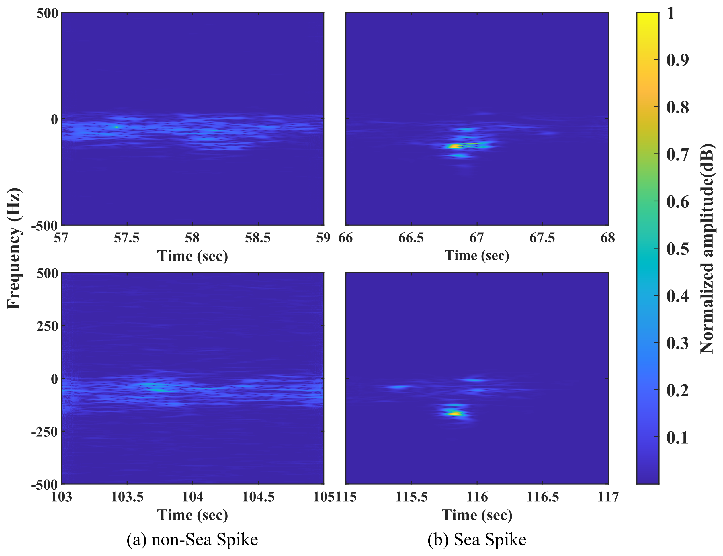
2.3. Time–Frequency Transforms of Radar Echoes

In this paper, we utilized primary target bin data and pure sea clutter bin data from #54 IPIX radar-measured data files in the same polarization mode. We extracted local continuous sampling data within a one-second interval, and performed time–frequency transformations using STFT, WVD, and SPWVD methods. According to Figure 1 and Figure 2, it is evident that slow-moving targets exhibit a linear feature in the time–frequency domain, with a concentrated energy distribution and minimal frequency variation within a short interval. In contrast, sea clutter demonstrates a scattered energy distribution, and occupies a broader frequency range. Additionally, it is evident that the clutter intensity in the primary target bin is insignificant when using the SPWVD method, demonstrating its strong capacity for clutter suppression. As SPWVD reduces cross-term interference, it provides higher time–frequency resolution than STFT and WVD. This creates notable distinctions in the time–frequency domain between target and sea clutter, making SPWVD suitable in the field of target detection against the background of sea clutter.

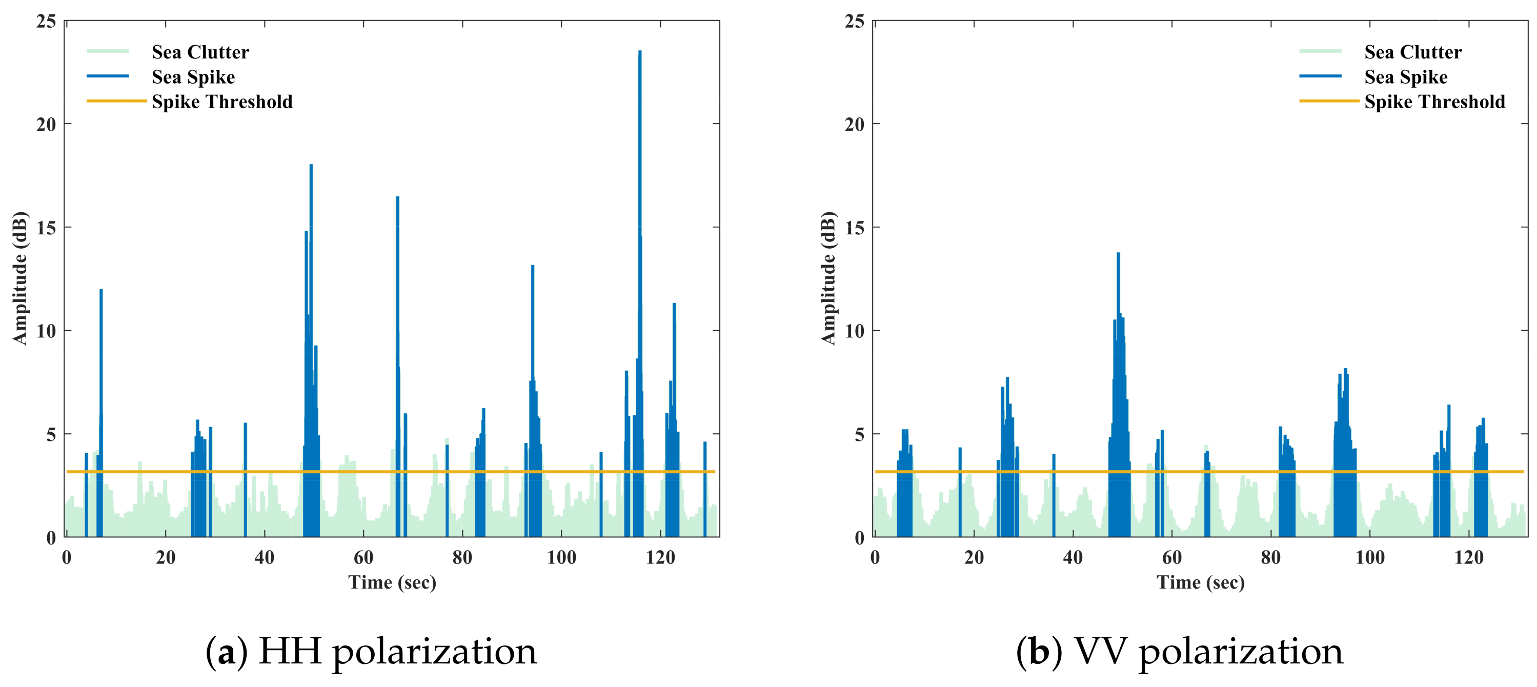
2.4. Sea Spike Determination

With improvements in radar resolution, an increasing amount of radar echo information from the sea surface is being obtained. Extensive experimentation and research have revealed that, when high-resolution radar detects the sea surface at relatively low grazing angles, the irregular motion and intense collisions of sea waves generate a significant number of breaking waves. After receiving the echo signals scattered by these breaking waves, the radar exhibits a long tail on the corresponding probability density function (PDF) curve [20], which is recognized as a sea spike. These sea spikes are randomly distributed at varying distances and angles throughout the radar echo map. These spikes have a short duration, but display strong fluctuations in scattered echo, causing a significant increase in the overall echo signal strength. This, in turn, increases the non-stationary and time-varying features of sea clutter. Additionally, certain high-intensity sea spikes resemble real targets, which increases the likelihood of radar systems misidentifying them during detection and raising a false alarm. This significantly impacts radar target detection performance.

To effectively analyze the temporal characteristics exhibited by sea spikes, it is first necessary to detect and identify the presence of sea spikes in radar echo signals. Posner [21] proposed a method for identifying sea spikes against the background of sea clutter. This discrimination method consists of three criteria. Firstly, the amplitude of the clutter sampling point should be relatively high, and must exceed a preset spike amplitude threshold, which is denoted by $T_d$. Secondly, a duration analysis is performed on clutter samples that meet the first criterion, and the continuous duration of clutter sampling points cannot be less than the set minimum spike width, which is denoted $W_{min}$. Lastly, the time between adjacent continuous clutter sampling points that meet the second criterion should be greater than the set minimum spike interval, denoted by $I_{min}$. These definitions are as follows:

$$\left\{\begin{array}{c}{\left|x_i\right|}^2\ge T_d\hfill \\ W_s\ge W_{min}\hfill \\ I_s\ge I_{min}\hfill \end{array}\right.$$

(12)

where $x_i$ represents the i-th sample point of the radar echo signal to be detected, $W_s$ represents the width of the sea spike, and $I_s$ represents the interval of the sea spike. The units of both $W_s$ and $I_s$ are in seconds. Assuming that the length of the radar echo signal x is N, the amplitude threshold value $T_d$ for sea spike peaks can be computed using the following equation:

$$T_d=\frac{L}{N}\sum _{i=1}^N{\left|x\left(i\right)\right|}^2$$

(13)

where L represents the multiple of the average signal power.

In practical applications, the existence of sea spikes within a specific range must satisfy the above three conditions. Moreover, sea spike discrimination criteria parameter values must be adjusted as the sea surface environment and radar observation parameters change.

The first bin data range of file #17 in the data measured using the IPIX radar was selected for experiments to distinguish and detect sea spikes in sea clutter data. The preset parameter values [22] during the experiment were $L=5$, $W_{min}=0.1$ and $I_{min}=0.5$. Figure 3 presents the sea spike detection results in various polarization modes.

In Figure 3, clutter data that are not sea spikes are represented in green, while the detected sea spike data are represented in blue. According to Figure 3, the amplitude of the sea spikes is greater than that of non-sea spike clutter. The amplitude of the non-sea spike clutter mostly remains below the threshold value $T_d$, and demonstrates relatively small fluctuations. In contrast, the amplitude of the sea spikes exhibits extremely pronounced fluctuations. Additionally, sea spikes display varied characteristics under different polarization modes. Sea spikes have a higher amplitude in horizontal–horizontal (HH) polarization mode compared to vertical–vertical (VV) polarization mode, and their duration is relatively short.

To explore the characteristics of sea spikes in the time–frequency domain, the SPWVD method was employed for the time–frequency transformation of both sea spike data and non-sea spike clutter data. Figure 4 illustrates the local SPWVD time–frequency distributions of non-sea spike clutter and sea spikes within different time intervals.

From Figure 4, it can be observed that there are significant differences between Figure 4a, the non-sea spike clutter, and Figure 4b, the sea spikes, in the time–frequency domain. Sea spikes often exhibit a larger Doppler shift than non-sea spikes, resulting in a wider spectrum. This is due to the breaking waves on the sea surface having relatively high velocities. Additionally, sea spikes exhibit a high energy density, severely masking the energy of non-sea spikes at other times, making their time–frequency distribution less apparent. This indicates that sea spikes have a greater echo intensity. Compared to non-sea spikes, sea spikes have a shorter duration and longer intervals between them, suggesting that the breaking waves dissipate quickly. Furthermore, both types of clutter exhibit temporal variations in frequency and energy, demonstrating the non-stationary nature of sea clutter. By comparing the performance of sea spikes and targets in the time–frequency domain, it can be inferred from Figure 1c and Figure 4b that targets exhibit longer durations over short time intervals than sea spikes.

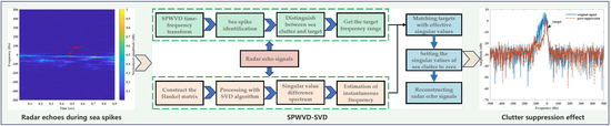
3. SPWVD-SVD Sea Clutter Suppression Algorithm

The pseudo-code of Algorithm 1 used for the sea clutter suppression method based on SPWVD-SVD is as follows:

Algorithm 1: Pseudo-code of the SPWVD-SVD algorithm.

The main procedures of the sea clutter suppression method using SPWVD-SVD are as follows. Firstly, apply the SPWVD method from the time–frequency analysis to transform the radar echo signal. Then, based on the time–frequency characteristics of sea spikes, the determination of sea spikes and targets is carried out to distinguish targets from clutter. This provides the frequency range of target components as it varies over time. Simultaneously, the echo signal is transformed into a Hankel matrix, and after SVD processing, matrix rank reduction is performed using the singular value difference spectrum method to estimate the instantaneous frequency of the signal components. Subsequently, a comparison is made with the target component frequencies in the time–frequency domain to obtain the instantaneous frequencies of the target components using the SVD algorithm. The corresponding singular values are retained, while the singular values corresponding to sea clutter are set to zero. Finally, the echo signal is reconstructed.

An overall flowchart of the SPWVD-SVD method is shown in Figure 5, as illustrated below.

3.1. Target and Sea Spike Determination

The SPWVD time–frequency transform is performed on the radar echo signal, and the frequency range of the target is determined based on the linear features exhibited by the target in the time–frequency domain. Considering the possibility of high-energy sea spikes that may be similar to the target and can lead to false alarms, a threshold $T_0$ is set, and sea spikes and targets are determined using the following equation:

$$\left\{\begin{array}{c}{T}_s\ge T_0,\mathrm{target}\hfill \\ T_s<T_0,\mathrm{sea}\mathrm{spike}\hfill \end{array}\right.$$

(14)

where $T_s$ represents the duration of the signal component.

3.2. Singular Value Difference Spectrum

By performing matrix rank reduction and discarding the insignificant singular values within the signal, the computational complexity of subsequent steps is reduced. Due to the non-stationary nature of sea clutter components, it is no longer feasible to assess effective singular values solely based on the number of narrowband signals. In this study, we employed the concept of singular value difference spectra in the field of signal denoising to effectively select significant singular values. The key lies in identifying the positions in which the singular values of the signal undergo abrupt changes. Suppose that, in a singular value difference spectrum b, the value of b represents the trends of change between adjacent singular values. Its definition is as follows:

$$b_i={\sigma }_i-{\sigma }_{i+1}i=1,2,\cdots ,l-1$$

(15)

If there is a significant difference between two adjacent singular values, there will be a large difference, resulting in sharp peaks at the corresponding positions in the difference spectrum. Let the position of the maximum mutation be denoted k, and the corresponding maximum peak point be denoted $b_k$. This position can be used to distinguish the singular values of signal and noise. If $k=1$, the presence of a certain direct current (DC) component in the measured signal is indicated, and the search for the next maximum mutation position, denoted by k, should continue. At this point, the number of effective singular values is the first k.

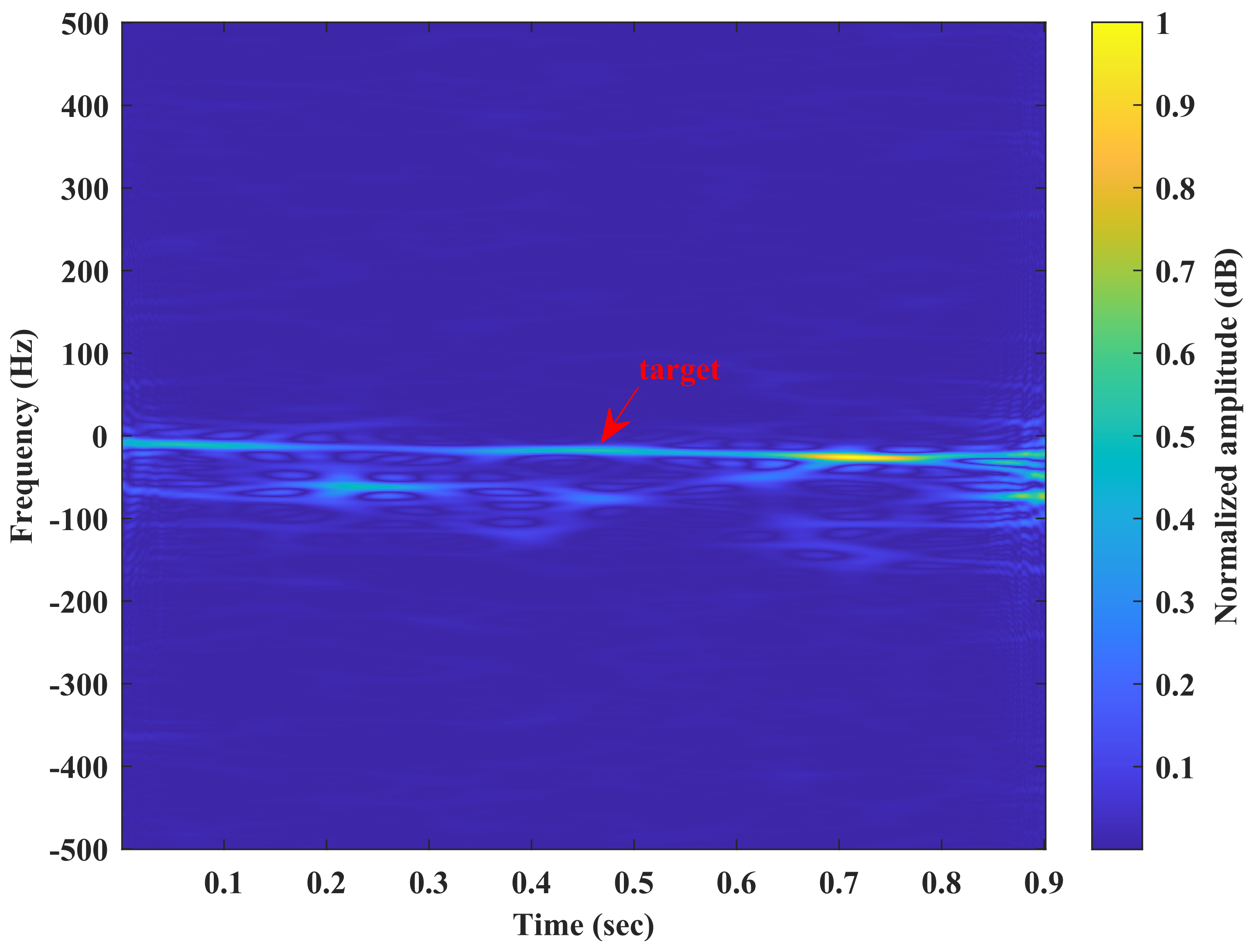
3.3. Estimating Target Frequency

Estimating the instantaneous frequencies of effective singular values after singular value decomposition allows us to capture the slow temporal variations in the frequencies of individual signal components. Subsequently, singular values corresponding to sea clutter can be determined by analyzing the instantaneous frequencies of signal components, thereby enabling the suppression of sea clutter.

Let the matrix ${\mathit{H}}_1$ after rank reduction be denoted

$${\mathit{H}}_1={\mathit{U}}_1{\mathit{S}}_1{\mathit{V}}_1^T$$

(16)

where ${\mathit{S}}_1=diag\left[{\sigma }_1,{\sigma }_2,\cdots ,{\sigma }_r\right]$.

Let the observation matrix $\tilde{\mathsf{\Gamma }}={\mathit{U}}_1{\mathit{S}}_1^{1/2}$, and divide $\tilde{\mathsf{\Gamma }}$ into multiple submatrices with row sizes equal to d, where d is the average of C, C denotes the number of columns $(C\in [3r$, int$[N/2]\left]\right)$, and r represents the narrowband signal number of $s\left(n\right)$. The following equation can be obtained:

$${\tilde{\mathsf{\Gamma }}}_k=\tilde{\mathsf{\Gamma }}(k:k+d,:)k=1,2,\cdots ,N-C+1-d$$

(17)

From the relationship between the matrix $\tilde{\mathsf{\Gamma }}$ and $\mathit{F}(d+k)$ [23], we obtain

$${\tilde{\mathsf{\Gamma }}}_k\mathit{F}(d+k)\cong {\tilde{\mathsf{\Gamma }}}_{k+1}k=1,2,\cdots ,N-C-d$$

(18)

where $\mathit{F}(d+k)$ represents the state feedback matrix, which can be determined using the least-squares method to solve the above equation. The definition of $\mathit{F}(d+k)$ is as follows:

$$\mathit{F}(d+k)=diag\left[e^{j{w}_1(d+k+1)},e^{j{w}_2(d+k+1)},\cdots ,e^{j{w}_r(d+k+1)}\right]$$

(19)

It can be seen from the above equation that $\mathit{F}(d+k)$ contains the instantaneous frequency of the signal. By calculating the eigenvalues of $\mathit{F}(d+k)$ and then obtaining the corresponding angles, the frequencies $f\left(n\right)$ of the signal at various moments can be determined:

$$f\left(n\right)=angle\left\{\mathrm{eigen}\right[F\left(n\right)\left]\right\}n=1,2,\cdots ,r$$

(20)

4. Experiments and Discussion

4.1. IPIX Data Sources

The data used in this paper were obtained from ten sets of measurements within the IPIX radar target database of 1993. During data collection, the radar was positioned on a cliff approximately 30 m high near the eastern coast of Canada, facing the Atlantic Ocean. The target to be detected was a floating spherical ball with a diameter of 1 m, wrapped in aluminum foil. The radar operates at a frequency of 9.3 GHz, with a beamwidth of 0.9 degrees and a range resolution of 30 m. The radar operated in a staring mode, with a pulse repetition frequency (PRF) of 1000 Hz and a dwelling time of approximately 131 s. Each dataset consisted of 14 range bins. The range bin with the strongest target signal is referred to as the primary range bin. Since the radar illuminates the target with a low grazing angle, the target fluctuation and swing lead to the diffusion of target energy, and distance oversampling is adopted during data acquisition. Therefore, the bin adjacent to the target bin will be affected by the target energy, which is recorded as the secondary range bin. Other range bins are typically considered pure clutter bins. The IPIX radar can transmit electromagnetic waves with horizontal and vertical polarization, and can utilize two linear receivers to achieve horizontal reception and vertical reception. Therefore, during radar data acquisition, it is typically possible to obtain radar echo data with four different polarizations: HH, VV, HV, and VH. Wind speed and wave height data for the year 1993 were obtained from environmental records during online data collection, with detailed information given in

Table 1. IPIX radar data collected in 1993.

Data Name	Wave Height (m)	Wind Speed (km/h)	Primary Bin	Secondary Bin
#17	2.2	9	9	8, 10, 11
#26	1.1	9	7	6, 8
#30	0.9	19	7	6, 8
#31	0.9	19	7	6, 8, 9
#40	1.0	9	7	5, 6, 8
#54	0.7	20	8	7, 9, 10
#280	1.6	10	8	7, 9, 10
#310	0.9	33	7	6, 8, 9
#311	0.9	33	7	6, 8, 9
#320	0.9	28	7	6, 8, 9

.

4.2. Verification of the SPWVD-SVD Suppression Algorithm

In this section, we first conduct experiments on sea clutter suppression using the SPWVD-SVD method with simulated targets. Pure sea clutter data are selected from the second range bin of file #17, specifically choosing a segment containing sea spikes. The simulated signal is a linear frequency-modulated (LFM) signal, with its frequency located within the spectrum of sea clutter. The target is designed to exhibit slight frequency variations over a short duration. Time-domain and frequency-domain representations of the target mixed with sea clutter are presented in Figure 6.

The suppression of clutter in the simulated signals was performed using wavelet transform and empirical mode decomposition (EMD) reconstruction methods [24], as shown in Figure 7. Due to the spectral overlap of the target within the broad spectrum of sea clutter, conventional denoising methods are no longer capable of distinguishing the frequency range of the target. Therefore, the two denoising methods mentioned above cannot effectively suppress clutter signals while preserving the target signal.

Upon performing the SPWVD time–frequency transformation on this signal, as shown in Figure 8, linear features emerge in the time–frequency distribution that resemble a target. After applying a threshold [25], denoted by $T_0=0.3$ s, it can be inferred that there is a target within this signal with a frequency range of approximately −25 Hz∼−5 Hz.

Figure 9 shows the singular value difference spectrum constructed after singular value decomposition. In the figure, the maximum peak of the singular value difference spectrum is located at position 1, indicating the presence of a DC component in the original signal. Continuing the search for the second maximum peak, as the second maximum peak is not significantly greater than the third maximum peak, the last abrupt change position of the singular value difference spectrum (which is at position 10 [26]) is chosen as the number of effective singular values for matrix rank reduction.

Calculating the instantaneous frequencies of the first ten effective singular values, Figure 10 shows the frequency range of the ten effective signal frequency components obtained via instantaneous frequency estimation. The approximate interval range for each frequency can be discerned from Figure 10. In many cases, the sum of the top 10% or even 1% of the singular values accounts for over 99% of the total sum of singular values. In other words, we can also use the top few singular values to approximate a description of the matrix [27]. To represent the singular values of the target signal, we select the top three frequencies within the range of −25 Hz∼−5 Hz. The frequency curve highlighted in orange represents the final selection of three frequencies that represent the effective singular values.

Figure 11a shows the frequency distribution of each effective singular value, with the red rectangular box indicating the target frequency range obtained via SPWVD. Figure 11b shows the probability that the instantaneous frequency of each effective singular value lies within the target frequency range.

Statistical analysis reveals that, for the majority of sampled points, the frequency of $\mathrm{f}5$, $\mathrm{f}6$, $\mathrm{f}7$ falls within the target frequency range identified by the SPWVD time–frequency analysis. Therefore, it can be considered that the singular value corresponding to $\mathrm{f}5$, $\mathrm{f}6$, $\mathrm{f}7$ is the singular value of the target, and these curves are highlighted in orange. In preserving the singular values of the target and setting the singular values of other signal components to zero, the spectral diagram of the reconstructed signal, as shown in Figure 12, clearly indicates the 4 effective suppression of sea clutter and the preservation of the target information within the spectral bandwidth.

The suppression results obtained using the traditional SVD suppression algorithm are shown in Figure 13a. While the traditional SVD algorithm suppresses some sea clutter components, it also filters out a proportion of the target components, resulting in a higher rate of missed alarms and false alarms. As shown in Figure 13b, through the SPWVD-SVD method, the sea clutter components in the time–frequency domain are effectively suppressed, enabling the more accurate extraction of information from weak targets. Additionally, it is possible to observe that the weak target is in a mode of slow motion.

After verifying the suppression effect of the SPWVD-SVD algorithm using a simulated signal, sea clutter suppression experiments using the SPWVD-SVD method were conducted with measurement data from the IPIX radar. For this experiment, the #17 file was selected, which corresponds to sea conditions with an effective wave height exceeding 2 m. The 9th range bin was chosen as the primary target bin, within which the target echo was most prominent. When the range bin experiences long-wave interference, sea spikes exhibit significantly broader frequency spectra in the frequency domain. At this time, the frequency of a target can be easily submerged. Sea-spike data with a time duration of one second were selected for the experiment, and their spectrum is shown in Figure 14a. It can be observed that the spectrum of the target is already mixed within the spectral width of the sea spike, and the frequency range of the target was indistinguishable. The SPWVD time–frequency transformation of this signal, as shown in Figure 14b, reveals linear features resembling the target in the signal’s time–frequency distribution. Additionally, there is more clutter interference in the time–frequency diagram when the sea spike takes effect.

A spectrogram of the signal after suppression and reconstruction using the SPWVD-SVD algorithm is shown in Figure 15a. It can be seen that the sea clutter has been effectively suppressed with an average clutter suppression of approximately 13.96 dB, while the target information within the spectral bandwidth has been preserved. Figure 15b shows a segment of the pure target signal, without sea spikes, extracted over a certain period of time. It can be observed that this signal is essentially consistent with the signal in Figure 15a after clutter suppression.

The results of the suppression of radar signals using the conventional SVD suppression algorithm are shown in Figure 16a. Similarly to the suppression of simulated targets, the traditional SVD algorithm suppresses some of the sea clutter components, but a significant degree of clutter signal is still present. The results obtained using the SPWVD-SVD suppression algorithm are depicted in Figure 16b, wherein the sea clutter components in the time–frequency domain are effectively suppressed, thereby providing more accurate information about weak targets.

4.3. Suppression Effects under Different Sea Conditions

Sea clutter suppression experiments were conducted on the ten sets of IPIX-measured data, as detailed in Table 1. The clutter suppression effectiveness of the SPWVD-SVD algorithm under different polarization conditions for these ten sets of data was statistically analyzed, and the results are shown in Figure 17.

As shown in Figure 17, the SPWVD-SVD suppression method achieves an average suppression of 15.04 dB under various sea conditions. Specifically, in the HH polarization mode, the average clutter suppression amplitude is 16.10 dB, while in the VV polarization mode, the average clutter suppression amplitude is 13.98 dB.

5. Conclusions

This paper addresses the challenging problem of target detection against the background of sea spikes. Firstly, the fundamental principles of the SVD algorithm are introduced, which primarily involve zeroing the singular values of sea clutter to filter out sea clutter and obtain the desired target signal. Subsequently, an analysis of the characteristics of the measured sea clutter data in the time–frequency domain is conducted. It is observed that, in the time–frequency domain, the energy of the target is concentrated, the frequency varies slowly with time, and the target exhibits linear features in the time–frequency domain over a short period of time. In contrast, the energy distribution of sea clutter is more scattered, showing significant intensity fluctuations. By comparing different time–frequency analysis methods, it is concluded that the smoothed pseudo-Wigner–Ville distribution (SPWVD) method exhibits more pronounced differences in the local characteristics of the target and sea clutter, demonstrating superior time–frequency analysis performance. The characteristics of sea spikes in the time–frequency domain were studied based on SPWVD. Sea spikes exhibit high energy and relatively short durations, with a relatively long time interval between adjacent spikes.

Building on the aforementioned research, this paper presents a method for determining sea spikes and targets. To address the problem of the inaccuracy of the SVD algorithm in capturing the singular values of a target against the background of sea spikes, the SPWVD-SVD method is proposed for the task of sea clutter suppression. This method primarily utilizes the frequency range of the target in the time–frequency domain of SPWVD to match the instantaneous frequencies of signal components in SVD, in order to achieve the suppression of sea clutter. Finally, suppression experiments are conducted using simulated data alongside measured data from IPIX radar, demonstrating that the SPWVD-SVD method can effectively suppress sea clutter, with an average clutter suppression of 15.04 dB under different sea conditions.

Currently, there is limited research on the suppression of unimodal and wide-spectrum sea clutter based on the SVD algorithm. Extensive measurement data are required to support further in-depth investigations. When the spectral components of strong sea clutter overlap with those of the target in the frequency domain within the echo signal, the characteristics of the target become weaker after time–frequency transformation. The effectiveness of the SPWVD-SVD method in suppressing sea clutter is relatively suboptimal, and requires further optimization.

References

1. Shuwen, X.; Xiaohui, B.; Zixun, G.; Penglang, S. Status and prospects of feature-based detection methods for floating targets on the sea surface. J. Radars 2020, 9, 684–714. [Google Scholar]
2. You, H.; Yong, H.; Jian, G.; Xiaolong, C. An overview on radar target detection in sea clutter. Mod. Radar 2014, 36, 1–9. [Google Scholar]
3. Wang, H.; Kirlin, R.L. Improvement of high frequency ocean surveillance radar using subspace methods based on sea clutter suppression. In Proceedings of the Sensor Array and Multichannel Signal Processing Workshop, Rosslyn, VA, USA, 6 August 2002; pp. 557–560. [Google Scholar]
4. Khan, R.; Power, D.; Walsh, J. Ocean clutter suppression for an HF ground wave radar. In Proceedings of the CCECE’97. Canadian Conference on Electrical and Computer Engineering. Engineering Innovation: Voyage of Discovery. Conference Proceedings, St. John’s, NL, Canada, 25–28 May 1997; Volume 2, pp. 512–515. [Google Scholar]
5. Lu, K.; Liu, X.; Liu, Y. Ionospheric decontamination and sea clutter suppression for HF skywave radars. IEEE J. Ocean. Eng. 2005, 30, 455–462. [Google Scholar] [CrossRef]
6. Lu, X.; Sun, R. A study on clutter cancellation method based on modified Hankel matrix singular value decomposition. Mod. Radar 2012, 34, 19–26. [Google Scholar]
7. Chen, Z.; He, C.; Zhao, C.; Xie, F. Using SVD-FRFT filtering to suppress first-order sea clutter in HFSWR. IEEE Geosci. Remote Sens. Lett. 2017, 14, 1076–1080. [Google Scholar] [CrossRef]
8. Yan, Y.; Wu, G.; Dong, Y.; Bai, Y. Floating small target detection in sea clutter based on the singular value decomposition of low rank perturbed random matrices. In Proceedings of the 2021 IEEE 5th Advanced Information Technology, Electronic and Automation Control Conference (IAEAC), Chongqing, China, 12–14 March 2021; pp. 527–531. [Google Scholar]
9. Stankovic, L.; Thayaparan, T.; Dakovic, M. Signal decomposition by using the S-method with application to the analysis of HF radar signals in sea-clutter. IEEE Trans. Signal Process. 2006, 54, 4332–4342. [Google Scholar] [CrossRef]
10. Zuo, L.; Li, M.; Zhang, X.; Wang, Y.; Wu, Y. An efficient method for detecting slow-moving weak targets in sea clutter based on time–frequency iteration decomposition. IEEE Trans. Geosci. Remote Sens. 2012, 51, 3659–3672. [Google Scholar] [CrossRef]
11. Zhang, X.W.; Yang, D.D.; Guo, J.X.; Zuo, L. Weak moving target detection based on short-time fourier transform in sea clutter. In Proceedings of the 2019 IEEE 4th International Conference on Signal and Image Processing (ICSIP), Wuxi, China, 19–21 July 2019; pp. 415–419. [Google Scholar]
12. Li, Z.; Ye, H.; Liu, Z.; Sun, Z.; An, H.; Wu, J.; Yang, J. Bistatic SAR clutter-ridge matched STAP method for nonstationary clutter suppression. IEEE Trans. Geosci. Remote Sens. 2021, 60, 1–14. [Google Scholar] [CrossRef]
13. Hu, J.; Tung, W.W.; Gao, J. Detection of low observable targets within sea clutter by structure function based multifractal analysis. IEEE Trans. Antennas Propag. 2006, 54, 136–143. [Google Scholar] [CrossRef]
14. Guan, J.; Liu, N.B.; Huang, Y.; He, Y. Fractal characteristic in frequency domain for target detection within sea clutter. IET Radar Sonar Navig. 2012, 6, 293–306. [Google Scholar] [CrossRef]
15. Metcalf, J.; Blunt, S.D.; Himed, B. A machine learning approach to cognitive radar detection. In Proceedings of the 2015 IEEE Radar Conference (RadarCon), Arlington, VA, USA, 10–15 May 2015; pp. 1405–1411. [Google Scholar]
16. Callaghan, D.; Burger, J.; Mishra, A.K. A machine learning approach to radar sea clutter suppression. In Proceedings of the 2017 IEEE Radar Conference (RadarConf), Seattle, WA, USA, 8–12 May 2017; pp. 1222–1227. [Google Scholar]
17. Yan, Y.; Xing, H. Small floating target detection method based on chaotic long short-term memory network. J. Mar. Sci. Eng. 2021, 9, 651. [Google Scholar] [CrossRef]
18. Djebbari, A.; Reguig, F.B. Short-time Fourier transform analysis of the phonocardiogram signal. In Proceedings of the ICECS 2000. 7th IEEE International Conference on Electronics, Circuits and Systems (Cat. No. 00EX445), Jounieh, Lebanon, 17–20 December 2000; Volume 2, pp. 844–847. [Google Scholar]
19. Barbarossa, S.; Zanalda, A. A combined Wigner-Ville and Hough transform for cross-terms suppression and optimal detection and parameter estimation. In Proceedings of the ICASSP-92: 1992 IEEE International Conference on Acoustics, Speech, and Signal Processing, San Francisco, CA, USA, 23–26 March 1992; Volume 5, pp. 173–176. [Google Scholar]
20. Rosenberg, L. Sea-spike detection in high grazing angle X-band sea-clutter. IEEE Trans. Geosci. Remote Sens. 2013, 51, 4556–4562. [Google Scholar] [CrossRef]
21. Posner, F.L. Spiky sea clutter at high range resolutions and very low grazing angles. IEEE Trans. Aerosp. Electron. Syst. 2002, 38, 58–73. [Google Scholar] [CrossRef]
22. Greco, M.; Stinco, P.; Gini, F. Identification and analysis of sea radar clutter spikes. IET Radar Sonar Navig. 2010, 4, 239–250. [Google Scholar] [CrossRef]
23. Poon, M.W.; Khan, R.H.; Le-Ngoc, S. A singular value decomposition (SVD) based method for suppressing ocean clutter in high frequency radar. IEEE Trans. Signal Process. 1993, 41, 1421–1425. [Google Scholar] [CrossRef] [PubMed]
24. Lv, M.; Zhou, C. Study on sea clutter suppression methods based on a realistic radar dataset. Remote Sens. 2019, 11, 2721. [Google Scholar] [CrossRef]
25. Zuo, L.; Chan, X.; Lu, X.; Li, M. Decomposing sea echoes in the time-frequency domain and detecting a slow-moving weak target in the sea clutter. J. Xidian Univ. 2019, 46, 84–90. [Google Scholar]
26. Zhao, X.; Ye, B. Selection of effective singular values using difference spectrum and its application to fault diagnosis of headstock. Mech. Syst. Signal Process. 2011, 25, 1617–1631. [Google Scholar] [CrossRef]
27. Zhao, H.; Wu, H.; Li, J.; Zhang, H.; Wang, X. Dtree2vec: A High-Accuracy and Dynamic Scheme for Real-Time Book Recommendation by Serialized Chapters and Local Fine-Grained Partitioning. IEEE Access 2020, 8, 23197–23208. [Google Scholar] [CrossRef]
Figure 1. The results of radar echoes from target bin data under different time–frequency transformations: (ac) are two-dimensional diagrams of three time–frequency transformations; (df) are three-dimensional diagrams of three time–frequency transformations.
Remotesensing 15 05360 g001
Figure 2. The results of radar echoes from pure clutter bin data under different time–frequency transformations: (ac) are two-dimensional diagrams of three time–frequency transformations; (df) are three-dimensional diagrams of three time–frequency transformations.
Remotesensing 15 05360 g002
Figure 3. Sea spike determination results under HH and VV polarization: (a) Sea spike determination in horizontal polarization mode for both transmission and reception; and (b) sea spike determination in vertical polarization mode for both transmission and reception.
Remotesensing 15 05360 g003
Figure 4. Time–frequency diagrams of non-sea spike and sea spike clutter at different times: (a) time–frequency diagrams of non-sea spike clutter at 57–59 s and 103–105 s; and (b) time–frequency diagrams of sea spikes at 66–68 s and 115–117 s.
Remotesensing 15 05360 g004
Figure 5. Flowchart of the SPWVD-SVD suppression method.
Remotesensing 15 05360 g005
Figure 6. Time–domain and frequency-domain diagrams of the simulated signal: (a) time-domain diagram of the simulated signal; and (b) frequency-domain diagram of the simulated signal.
Remotesensing 15 05360 g006
Figure 7. Wavelet and EMD reconstruction suppression algorithm: (a) wavelet transform-weighted reconstruction; and (b) EMD reconstruction.
Remotesensing 15 05360 g007
Figure 8. Time–frequency transformation diagram of the signal simulated using SPWVD.
Remotesensing 15 05360 g008
Figure 9. Singular value difference spectrum.
Remotesensing 15 05360 g009
Figure 10. The frequency range of ten effective singular values.
Remotesensing 15 05360 g010
Figure 11. Estimation of singular value frequency: (a) the frequency distribution of ten significant singular values; and (b) probability of effective singular values within the signal frequency range. The orange component represents the singular values of the signal to be retained.
Remotesensing 15 05360 g011
Figure 12. Comparison between the original spectral diagram of the simulated signal and the suppressed spectral diagram.
Remotesensing 15 05360 g012
Figure 13. Time–frequency diagrams of different suppression algorithms: (a) Suppression of a simulated signal using the SVD algorithm; and (b) suppression of a simulated signal using the SPWVD-SVD algorithm.
Remotesensing 15 05360 g013
Figure 14. Spectrum and time–frequency diagram of the measured radar signal: (a) Spectrum diagram of the radar signal; and (b) time–frequency diagram of the radar signal.
Remotesensing 15 05360 g014
Figure 15. Comparison between the original spectral diagram of the measured radar target signal and the suppressed spectral diagram: (a) spectrum diagram of the radar signal; and (b) clean signal without sea spikes.
Remotesensing 15 05360 g015
Figure 16. Time–frequency diagrams of the radar target signal measured after the application of various suppression algorithms: (a) radar signal suppressed using the SVD algorithm; and (b) radar signal suppressed using the SPWVD-SVD algorithm.
Remotesensing 15 05360 g016
Figure 17. Clutter suppression results on different IPIX data.
Remotesensing 15 05360 g017