Abstract
This study carefully assesses the capability of supervised machine learning classification algorithms in identifying land cover (LC) in the context of the Jhelum River basin in Kashmir. Sentinel 2 and Landsat 8 high-resolution data from two satellite sources were used. Through preprocessing techniques, we removed any potential noise inherent to satellite imagery and assured data consistency. The study then utilized and compared the skills of the supervised algorithms random forest (RF) and support vector machine (SVM). A hybrid approach, amalgamating classifications from both methods, was also tested for potential synergistic enhancements in accuracy. Using a stratified random sampling approach for validation, the SVM algorithm emerged with a commendable accuracy rate of 82.5%. Using simulations from 2000 to 2015, the soil and water assessment tool (SWAT) model was used to further explore the hydrological effects of LC alterations. Between 2009 and 2019, there were discernible changes in the land cover, with a greater emphasis on ranges, forests, and agricultural plains. When these changes were combined with the results of the hydrologic simulation, a resultant fall in average annual runoff—from above 700 mm to below 600 mm—was seen. With runoff values possibly ranging between 547 mm and 747 mm, the statistics emphasize the direct effects of urban communities encroaching upon forest, agricultural, and barren lands. This study concludes by highlighting the crucial role that technical pipelines play in enhancing LC classifications and by providing suggestions for future water resource estimation and hydrological impact evaluations.
1. Introduction
Insights gained from modern environmental research and policymaking are increasingly dependent on cutting-edge technologies. Accurate land cover classification generated from satellite data has become a cornerstone of hydrology and river basin management [1]. However, as with many technologies, further research is needed to fully understand the advantages and drawbacks of satellite-derived classifications.
Launched in 2013 and 2015, respectively, Landsat-8 and Sentinel-2 have revolutionized the classification of land cover [2]. With unprecedented spatial and temporal resolutions, combined with their spectral capabilities, they furnish a platform to distinguish even subtle land cover types [3]. The ability of these satellites to provide complex land cover analysis opens the door to a wide range of applications, particularly in the management of water resources.
However, challenges arise when translating these classified data into tangible insights for river basins. River basins, which can cover large areas with a variety of land cover types, are essential to regional hydrological cycles. The hydrological responses of the basin are impacted by altered land cover patterns, which have an effect on evapotranspiration, soil moisture, and subsequently, runoff [4].
The soil and water assessment tool (SWAT), since its inception, has been a reliable tool to simulate the hydrological impacts of varied land use/land cover in expansive watersheds [5]. Its integration with satellite data aims at a precise hydrological simulation. Yet, the conundrum persists: how reliable are these simulations, especially given the dynamic nature of river basins?
The distinction between “land use” and “land cover” is a key problem. Turner et al. [6] point out that the latter is about the physical stuff on the surface, while the former pertains to the human application of the land (agricultural, urbanization, etc.). This distinction goes beyond simple semantics. Decisions about water management could potentially be impacted by misinterpretation, which can result in flawed modeling. With the increasing urban sprawl and agricultural intensification, land cover alterations are accelerating, potentially straining water resources in river basins [7].
Moreover, in a river basin, weather data have a significant impact on the quantity and quality of water [8,9,10,11]. The hydrologic model’s performance is improved through better estimation and prediction of weather and land cover characteristics [12,13,14]. The hydrologic model’s prediction is improved by appropriate geographical and temporal resolution of the used land cover and the better weather data [15,16]. Several easy-to-use and widely accessible spatial and weather datasets have been generated because of the increased availability of spatial information in watershed modeling [17,18,19].
However, determining which data source is superior and how data from diverse sources affect model outcomes is difficult [20]. In this research, stream flow findings in the Jhelum River Basin, Kashmir, from the soil and water assessment tool (SWAT) model using three distinct types of land cover datasets and two different weather datasets will be described. The study’s goal is to investigate how changing land cover affects the runoff from the reservoir due to precipitation. The study examines the interactions between the characteristics of land cover change (land cover types) and the hydrologic processes (water output and groundwater storage). The hydrologic process model SWAT was used to simulate the hydrologic effects of the land cover changes and results were recommended for future water resources management.
In conclusion, this study’s core goes beyond simple data analysis. It has the potential to change how we manage water resources in river basins. The findings from this study aim to open the door for more sustainable and well-informed decisions by closing conceptual gaps, resolving underlying difficulties, and improving techniques. The significance of such studies cannot be over-emphasized in a world where water scarcity and environmental uncertainty are on the rise. Finally, it clarifies the intricate dynamics of land cover while also highlighting the significant effects they have on our limited water supplies.
2. Materials and Methods
Situated in the heart of the expansive Indus Basin, our study area encompasses the Jhelum River Basin (JRB), which spans 33,397 km2, marking it as the second-largest tributary of the Indus Basin, see Figure 1 [21]. The Jhelum River Basin offers a unique confluence of varied topography, hydrological significance, and critical water resource management challenges, making it an ideal locale for comprehensive study.
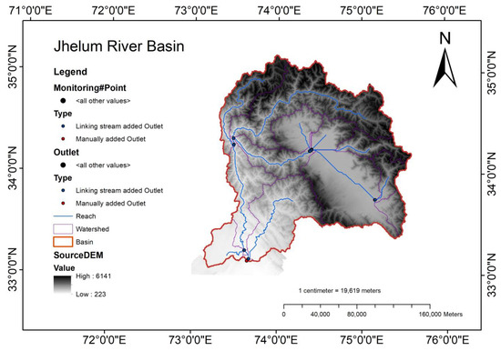
Figure 1.
Jhelum River Basin (Study Area).
2.1. Classification Algorithms
Machine learning algorithms (MLAs) have gained prominence in detecting variations in land cover (LC) primarily from a restricted range of imagery [22,23,24,25]. However, there is ongoing discussion in the literature over the temporal consistency of MLAs [26,27,28].
A supervised learning algorithm called the support vector machine (SVM) is used to resolve regression and classification problems [29]. SVM classifiers build an ideal hyperplane during the training phase that splits multiple classes with the fewest misclassified pixels. A SVM is used to choose the extreme points and vectors required to construct the hyperplane. These extreme areas are known as support vectors [30]. The cost element Kernel, gamma, and C functions are the main factors to consider while selecting support vectors [31]. The grid search method is used to define the C and Gamma parameters, yielding precise prediction results. The SVM and support vector machines’ performance are substantially impacted by the cost parameter C [32]. The linear kernel is preferred for training on large datasets.
The most often used classifier, random forest (RF), builds an ensemble classifier by combining many CART trees [33]. RF builds several decision trees using a random selection of training datasets and parameters. Internally, the classifier’s performance is evaluated together with an impartial assessment of the generalization error using the non-training instances [34]. RF randomly selects variables from training samples at each node to establish the best split for tree construction. The most important user-defined input parameter for RF is the number of parameters and trees. According to the research, between 100 and 500 trees should be counted, and the square of the set of variables should be used as the number of variables to count [35]. In this research, ArcGIS 10.4 was used for the classification of images by RF. For the classification purpose, 16 training samples were used against 16 classes.
In the current study, the above mentioned two classification methods—support vector machines (SVM) and random forest (RF)—were used to compare how accurate they were in classifying land cover of the Jhelum River Basin. To compare the performance of these supervised algorithms, both the satellite images were also classified by using the combined classification. This technique enables parallel monitoring of the classification process and class accuracy. ERDAS Imagine was used for combined classification.
2.2. Classification Assessment
In the post-classification phase, the veracity of images categorized through machine learning methodologies was ascertained. An accuracy assessment is instrumental in gauging the precision of the classified result, which mandates a reference dataset congruent to the classification schema. The most common method for performing such evaluations entails creating a random point set from ground truth data and comparing it to the categorized dataset in a confusion matrix. The four types of accuracy that were taken into consideration for this study are listed below.
where:
- P_Accuracy = the producer’s accuracy column shows false negatives, or errors of omission. The producer’s accuracy indicates how accurately the classification results meet the expectation of the creator.
- U_Accuracy = the user’s accuracy column shows false positives, or errors of commission, in which pixels are incorrectly classified as a known class when they should have been classified as something else.
- κ = Kappa Coefficient.
- C = Column Total.
- D = Row Total.
2.3. Hydrologic Model
The soil water assessment tool (SWAT) model was developed as a distributed conceptual, physically based hydrologic model to predict the effects of land management practices on water, sediment, and agricultural chemical yield in substantial, complex watersheds with varying soil, land cover, and management conditions over extensive time periods [36].
where SWt is the final soil content of the water (mm), SWo is the initial soil water content on the ith day (mm), Rday is the amount of precipitation on the ith day (mm), Qsurf is the amount of surface runoff on the ith day (mm), Ea is the amount of evapotranspiration on the ith day (mm), Wseep is the amount of water entering the vadose zone on the ith day (mm) and Qgw is the amount of return flow on the ith day (mm). To determine the total sub-basins and basin values, the hydrologic processes listed in Equation (5) are anticipated independently for each hydraulic response unit (HRU). In other terms, the HRU is the operating unit of the model. To investigate the complex basin, the model divides it into several sub-basin units, each drained by a reach. Each sub-basin is further divided into an HRU (where hydrologic processes are seen as homogeneous) using a specific combination of land cover, soil type, and slope. The SWAT HRU water balance is made up of 16 storage volumes, including snow, a soil profile (0–2 m), a shallow aquifer (typically 2–20 m), and a deep aquifer (>20 m) [37].
2.4. Temporal Data
The SWAT model is developed to consider a range of modeling objectives as well as the quantity and caliber of accessible input data. Climate-related variables are either generated by a custom weather generator or incorporated into the SWAT model using historical data [38]. The climate data for 15 years (2000–2015) were obtained by the SWAT global weather database for JRB (https://swat.tamu.edu/data/cfsr (accessed on 17 April 2020)). The soil data were obtained by the SWAT global weather database under the title India datasets, which includes data for not only India but for the whole world data by FAO (Food and Agriculture Organization) (https://swat.tamu.edu/data/(accessed on 1 July 2020)). Three types of land cover data were used in this research. First was obtained by global land cover 2009 (http://due.esrin.esa.int/page_globcover.php (accessed on 1 January 2021)). The digital elevation model for the study area at 30 m resolution, 2019 Landsat 8 and Sentinel 2 image was downloaded from the USGS website (https://www.usgs.gov/landsat-missions/landsat-8 (accessed on 13 January 2021)) and the bands with 30 m resolution for Landsat 8 and with 10 m resolution from Sentinel 2 were used to prepare the target study area which in this case was the Jhelum River Basin (JRB).
2.5. Application Framework
Utilizing Landsat-8 and Sentinel-2 satellite data, land cover images of the Jhelum River Basin were generated. The classification was carried out using two primary algorithms: a support vector machine (SVM) and random forest (RF). To ensure a comprehensive analysis, both satellite images underwent a combined classification technique. Following this, an accuracy assessment was conducted, comparing the classified images with a reliable reference dataset, which in this case was a high-resolution imagery. To compare the classification map’s accuracy, random points from the reference dataset were mapped into a confusion matrix. ArcGIS 10.4 was used to carry out the full procedure. Following categorization, the SWAT model was used to investigate the hydrological effects, providing information about how land cover has changed over time.
3. Results
3.1. Land Cover Classification
Figure 2 shows the classified images of Landsat 8 and Sentinel 2 satellite images. The total number of classes is 16 and their names can be seen in Table 1, while SWAT codes can be seen in the legend of Figure 2. From the visual inspection, the random forest classified Landsat 8 image depicts more pixels in the red color which means that it is overestimating the urban settlements (Figure 2b). Such a kind of error is a thematic error, which occurs when a training sample for a certain class includes a pixel or number of pixels of other classes, and during the classification a supervised algorithm using that sample confuses all the classes. The error is smaller in the case of support vector machines (Figure 2a) due to the difference in the classification methods of support vector machines and random forest. Calculated areas of different land-use classes for Landsat 8 classified image are reported in Table 1.
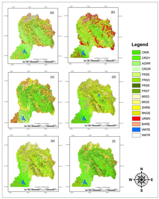
Figure 2.
(a) SVM Classified Landsat 8 Image; (b) Random Forest Classified Landsat 8 Image; (c) Combine Classified Landsat 8 Image; (d) SVM Classified Sentinel 2 Image; (e) Random Forest Classified Sentinel 2 Image; (f) Combine Classified Sentinel 2 Image. Details of legend is explained in Table 1.

Table 1.
Land cover Area of different classes for Landsat 8 image classified by different algorithms.
From Table 1, it can be seen that the area is mostly made up of rain-fed and dry crops. The rain-fed crops area for different algorithms is 5982.5 km2 by support vector, 4822.7 km2 by random forest and by combined classification it is 24.5 km2. Dry crops, on the other hand, constituted a land use of 6985.7 km2 (highest value). The remaining land uses are reported in Table 1. From Table 2, it can be seen that the areas in the case of Sentinel 2 image are surprisingly different from the classified Landsat 8 image. In most of the cases, the areas are greater than the areas from the Landsat8 classified image. The greatest area values are for herbaceous land: they are 9454.8 km2 by support vector and 7538.7 km2 by random forest, respectively. In addition, the greatest value is also for herbaceous land. The rest of the values can be seen in Table 2. The comparison of values for the two satellite images is reported in Table 2.
Table 2.
Land cover area of different classes for Sentinel 2 image classified by different algorithms.
3.2. Accuracy Assessment
For the Landsat 8 image classification, accuracy reports were created, and a summary of the classification accuracy is reported in Table 3. Overall classification accuracy for support vector machines was found to be 82.5% and the kappa coefficient was 81.33%. For random forest, the decrease in accuracies can be observed due to the thematic error and the values are 64% for kappa and 66% for overall accuracy. In the case of the Sentinel 2 image (Table 4), the accuracies were high for the random forest algorithm with a value of 78% for overall accuracy and kappa coefficient. A comparison was made between the land-use areas of global land cover 2009 and 2019 Landsat 8 classified image with the greatest accuracy achieved from the classification methods considered in this research. The area showed the highest rate in terms of urbanization with a value of 4232.9 km2 as compared to the urban area calculated by global land cover in 2009 which was 14. km2. Despite achieving high classification accuracy, the support vector machines exhibited some misclassification, particularly in urban areas, suggesting potential confusion between urban pixels and other classes, leading to potentially erroneous results. The remaining classes did not depict this difference and the values for these classes were acceptable. Larger areas include ranges, forests, and agriculture with the values of 7215.6 km2, 6443.5 km2 and 13,333.1 km2, which are lesser than the areas of global land cover in 2009. Most classes showed a decreasing trend, but settlements skyrocketed during the 10 years between 2009 and 2019 (Figure 3).
Table 3.
Accuracy assessment of Landsat 8 classified image.
Table 4.
Accuracy assessment of Sentinel 2 classified image.
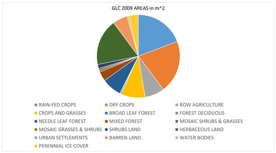
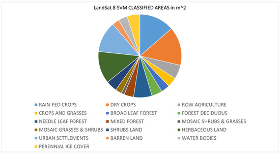
Figure 3.
Areal Coverage Comparison between Global Land cover 2009 and SVM classified Land Cover 2019.
3.3. Hydrologic Simulations
A comparative analysis was conducted to examine the impact of variations in the land use areas within the Jhelum River Basin, as discerned from the global land use data of 2009 and a 2019 Landsat 8 classified image, noted for its elevated accuracy values, on the hydrological simulations crafted via the SWAT model. Figure 4, Figure 5, Figure 6, Figure 7, Figure 8, Figure 9, Figure 10 and Figure 11 articulate the average monthly values for assorted components of the hydrologic cycle, revealing discernible fluctuations in both surface and lateral runoff, along with sediment yield, while concurrently maintaining consistent trends across the remaining components.
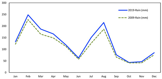
Figure 4.
Rainfall Comparison for Simulations of Land Cover 2009 and Land Cover 2019.
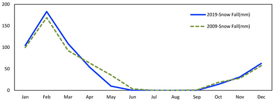
Figure 5.
Snowfall Comparison for Simulations of Land Cover 2009 and Land Cover 2019.
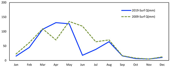
Figure 6.
Surface Runoff Comparison for Simulations of Land Cover 2009 and Land Cover 2019.
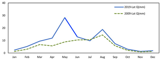
Figure 7.
Lateral Runoff Comparison for Simulations of Land Cover 2009 and Land Cover 2019.
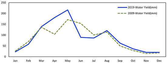
Figure 8.
Water Yield Comparison for Simulations of Land Cover 2009 and Land Cover 2019.
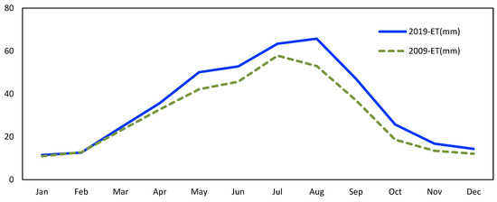
Figure 9.
Evapotranspiration Comparison for Simulations of Land Cover 2009 and Land Cover 2019.
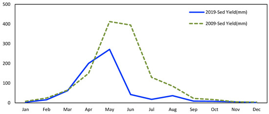
Figure 10.
Sediment Yield Comparison for Simulations of Land Cover 2009 and Land Cover 2019.
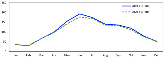
Figure 11.
Potential Evapotranspiration Comparison for Simulations of Land Cover 2009 and Land Cover 2019.
3.4. Sensitivity Analysis
Figure 12 depicts the effect of land-use classes on the surface runoff of a river basin. The runoff obtained by a classified JRB satellite image was 596.33 mm and the curve number (that is an infiltration parameter dependent on the assumed land use/land cover scenario, ranging from 0, all the rainfall becomes infiltration, and no runoff is present, to 100, all the rainfall becomes runoff and no infiltration is present) obtained was 78.01 (Figure 13). Interchange of classes indicated that the larger forest area decreased the surface runoff to nearly 540 mm. Conversely, the presence of larger urban areas increased the runoff to 740 mm, which explains the increase in runoff by 200 mm from the original value. The rest of the values can be seen in Figure 12. From the Figure, we can observe the scenarios in which other classes, if converted to urban settlements, added volume to the runoff. For example, in the case of agricultural land to urban settlement the value is 635.4 mm and interchange of ranges and urban settlements recorded 662.37 mm (Figure 12). The curve number (CN) derived from the classified satellite imagery of the Jhelum River Basin was quantified as 78.01, wherein a lower CN indicates a diminished runoff. Analyzing Figure 13 reveals a nuanced relationship between land cover type and CN: an increased forest land proportion led to a reduced CN of 75.1, while an augmentation of urban areas elevated the CN to a notable 82.73. This underscores a discernible relationship where a proliferation of forested lands mitigates the runoff to the river basin, while, conversely, urbanization amplifies it.
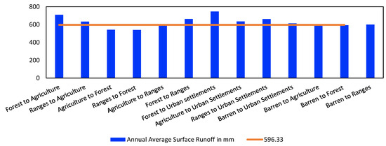
Figure 12.
Impact of Land-cover Classes on Surface Runoff.
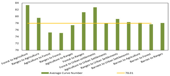
Figure 13.
Impact of Land-cover Classes on Curve Number.
4. Discussion and Conclusions
The findings revealed that the support vector method exhibited exceptional classification performance, achieving an accuracy rate exceeding 80% when applied to image data. In the context of thematic errors, the utilization of the random forest algorithm led to a notable reduction in the accuracy levels of the classified images, plummeting to nearly 60%. This decline in accuracy was primarily attributed to the higher prevalence of cloud cover in Sentinel-2 images compared to Landsat 8 images. Interestingly, while this increased cloud cover posed challenges for the support vector classifier, it appeared to have a more favorable impact on the performance of the random forest method, resulting in relatively greater accuracy outcomes.
In the case of Sentinel-2 data, the greatest achievable accuracy remained below the 80% threshold. When it came to Landsat 8 data, combined classification yielded commendable results, surpassing 75%, but disappointingly, this approach performed poorly when applied to Sentinel-2 imagery, resulting in a substantial drop in accuracy to 65%.
To assess changes in the water balance cycle within the Jhelum River Basin, a series of simulations spanning 15 years (2000–2015) were conducted using a combination of Landsat 8 SVM-classified images and the global land use data from 2009. These simulations revealed significant variations in surface and lateral runoff as well as sediment yield, while other components demonstrated relatively consistent trends. Notably, the analysis indicated that the conversion of forested areas, agricultural zones, rangelands, and barren lands into urban settlements could potentially elevate the average annual runoff from 596 mm to a striking 747 mm. Conversely, an increase in forested regions had the potential to decrease the annual runoff to as low as 547 mm from its previous level of nearly 600 mm. The results are in line with the previous literature. For instance, Recanatesi and Petroselli [39] found that urbanization increases the flood risk, which was more pronounced in the part of the selected area that has been more extensively interested by the soil sealing. Kandissounon et al. [40] quantified the contribution of extensive land cover change to urban flooding in Nigeria, describing an urban area where the changes in land cover led to a 64% increase in average surface runoff for single rainfall events, and an average annual surface runoff that has almost doubled due to amplified soil imperviousness. Umukiza et al. [41] evaluated the peak discharge and flow volume under different assumed scenarios of land use/land cover projected starting from a diachronic analysis of satellite images from 1985 and 2019. The results showed that the peak discharge and flow volume are affected by the variation in the CN value. Vojtek and Vojteková [42] in order to estimate the surface runoff for a watershed in Slovakia, in their investigated period (1949–2017), observed quite significant changes due to land cover changes, with arable land decreasing the most, by more than half, while the share of forests increased. In these circumstances, the runoff volume values in the basin area decreased during the years covered. Finally, it is noteworthy that land cover changes affect not only the surface water runoff, but are also a key input in environmental evaluations for the sustainable planning and management of socio-ecological systems, as demonstrated by Pelorosso et al. [43].
Therefore, in conclusion, for JRB changes in land cover areas do affect the runoff, the precise calculation of which is necessary for sustainable water resource quantification in a multi-purpose river basin.
Research Innovation and Future Recommendations
Our investigation transcends mere computational application, delving into a nuanced exploration of the interplay between varying algorithmic applications and their ramifications on land cover classification, particularly within the nuanced geographic context of the Jhelum River Basin. Distinct algorithms exhibit varied efficacies across divergent satellite data, a paradigm explicitly illustrated in the comparative analysis between the support vector machine (SVM) and random forest (RF) approaches. The SVM, albeit sensitive to sample selection, showcased adeptness in navigating the intricate geography, enabling precise classification of obscured or intermingled classes. In contrast, RF demonstrated a less proficient management of geographic complexity, underscoring the necessity for algorithmic selection to be intricately tied to data characteristics and the research context.
Furthermore, it became clear that the clarity and purity of satellite data were crucial for successful classification, with impurities or cloud obfuscations having the potential to cause pixel amalgamation and, as a result, class confusion during the classification process. This reveals a crucial point for further study and applications in water management, notably in determining the effects of changing land cover on hydrological simulations using SWAT-like models. The findings’ elucidation of the quantifiable impact of various land use classes on runoff provides water managers with data-driven insights that enable a more comprehensive and flexible strategy for quantifying and allocating water resources.
This study advocates for the strategic integration of these methodologies in water resource quantification, particularly in conjunction with physically parameterized hydrologic models like SWAT. This is because land-cover classes have a significant impact on river basin runoff and classification algorithms have been shown to be accurate. It is a project that goes beyond simple quantitative analysis and navigates the many fluidities and complexities of water management, which are intricately linked to shifting land-use patterns and environmental factors.
Considering the lessons learned from the Jhelum River Basin, future research directions should focus on improving the combination of machine-learning algorithms and hydrological models. This involves putting special emphasis on supporting various geographical resolutions and giving ongoing updates to land-cover and land-use datasets priority to improve prediction accuracy. Fostering collaborative interfaces between hydrologists and data scientists is crucial for the development of effective, flexible, and scientifically sound water management practices, especially in areas subject to changing hydrological patterns.
Author Contributions
Conceptualization, F.H. and S.K.; methodology, F.H.; software, R.F. and F.H.; validation, R.F. and F.H.; formal analysis, F.H.; investigation, F.H. and M.R.I.; data curation, F.H. and M.R.I.; writing—original draft preparation, F.H. and S.K.; writing—review and editing, A.P. and R.F.; supervision, S.K. and A.P. All authors have read and agreed to the published version of the manuscript.
Funding
This research received no external funding.
Data Availability Statement
Data are available on request.
Conflicts of Interest
The authors declare no conflict of interest.
References
- Petit, C.; Scudder, T.; Lambin, E. Quantifying processes of land-cover change by remote sensing: Resettlement and rapid land-cover changes in south-eastern Zambia. Int. J. Remote Sens. 2001, 22, 3435–3456. [Google Scholar] [CrossRef]
- Wulder, M.A.; Coops, N.C. Satellites: Make Earth observations open access. Nature 2014, 513, 30–31. [Google Scholar] [PubMed]
- Li, J.; Roy, D.P. A Global Analysis of Sentinel-2A, Sentinel-2B and Landsat-8 data revisit intervals and implications for terrestrial monitoring. Remote Sens. 2017, 9, 902. [Google Scholar] [CrossRef]
- Owe, M.; de Jeu, R.; Holmes, T. Multisensor historical climatology of satellite-derived global land surface moisture. J. Geophys. Res. Earth Surf. 2008, 113, F01002. [Google Scholar] [CrossRef]
- Gassman, P.W.; Reyes, M.R.; Green, C.H.; Arnold, J.G. The soil and water assessment tool: Historical development, Applications, and Future Research Directions. Trans. ASABE 2007, 50, 1211–1250. [Google Scholar] [CrossRef]
- Turner, B.L., II; Lambin, E.F.; Reenberg, A. The emergence of land change science for global environmental change and sustainability. Proc. Natl. Acad. Sci. USA 2007, 104, 20666–20671. [Google Scholar]
- Jensen, J.R.; Jensen, R.R. Introductory Geographic Information Systems; Pearson Higher Education: London, UK, 2012. [Google Scholar]
- Vivekananda, G.; Swathi, R.; Sujith, A. Multi-temporal image analysis for LULC classification and change detection. Eur. J. Remote Sens. 2021, 54, 189–199. [Google Scholar]
- de Mello, K.; Taniwaki, R.H.; de Paula, F.R.; Valente, R.A.; Randhir, T.O.; Macedo, D.R.; Hughes, R.M. Multiscale land use impacts on water quality: Assessment, planning, and future perspectives in Brazil. J. Environ. Manag. 2020, 270, 110879. [Google Scholar]
- Bao, Z.; Zhang, J.; Wang, G.; Chen, Q.; Guan, T.; Yan, X.; Liu, C.; Liu, J.; Wang, J. The impact of climate variability and land use/cover change on the water balance in the Middle Yellow River Basin, China. J. Hydrol. 2019, 577, 123942. [Google Scholar]
- Luo, Z.; Shao, Q.; Zuo, Q.; Cui, Y. Impact of land use and urbanization on river water quality and ecology in a dam dominated basin. J. Hydrol. 2020, 584, 124655. [Google Scholar]
- Stephens, C.; Marshall, L.; Johnson, F. Investigating strategies to improve hydrologic model performance in a changing climate. J. Hydrol. 2019, 579, 124219. [Google Scholar] [CrossRef]
- Farooq, R.; Mekanik, F.; Imteaz, M. Long Term Seasonal Rainfall Forecasting Using Artificial Neural Network: Case Study of Northern Territory, Australia. In Hydrology & Water Resources Symposium 2022 (HWRS): The Past, the Present, the Future; Engineers Australia: Brisbane, Australia, 2022; pp. 247–254. Available online: https://search.informit.org/doi/10.3316/informit.906134357228181 (accessed on 24 August 2023).
- Syed, Z.; Mahmood, P.; Haider, S.; Ahmad, S.; Jadoon, K.Z.; Farooq, R.; Ahmad, K. Short–long-term streamflow forecasting using a coupled wavelet transform–artificial neural network (WT–ANN) model at the Gilgit River Basin, Pakistan. J. Hydroinform. 2023, 25, 881–894. [Google Scholar] [CrossRef]
- Schaperow, J.R.; Li, D.; Margulis, S.A.; Lettenmaier, D.P. A near-global, high resolution land surface parameter dataset for the variable infiltration capacity model. Sci. Data 2021, 8, 216. [Google Scholar] [PubMed]
- Giuliani, G.; Rodila, D.; Külling, N.; Maggini, R.; Lehmann, A. Downscaling Switzerland land use/land cover data using nearest neighbors and an expert system. Land 2022, 11, 615. [Google Scholar] [CrossRef]
- Abatzoglou, J.T.; Dobrowski, S.Z.; Parks, S.A.; Hegewisch, K.C. TerraClimate, a high-resolution global dataset of monthly climate and climatic water balance from 1958–2015. Sci. Data 2018, 5, 170–191. [Google Scholar] [CrossRef] [PubMed]
- Ahmadisharaf, E.; Camacho, R.A.; Zhang, H.X.; Hantush, M.M.; Mohamoud, Y.M. Calibration and validation of watershed models and advances in uncertainty analysis in TMDL studies. J. Hydrol. Eng. 2019, 24, 03119001. [Google Scholar] [CrossRef]
- Rajib, A.; Kim, I.; Golden, H.; Lane, C.; Kumar, S.; Yu, Z.; Jeyalakshmi, S. watershed modeling with remotely sensed big data: MODIS leaf area index improves hydrology and water quality predictions. Remote Sens. 2020, 12, 2148. [Google Scholar] [CrossRef] [PubMed]
- Deng, Y.; Bartosovic, M.; Ma, S.; Zhang, D.; Kukanja, P.; Xiao, Y.; Su, G.; Liu, Y.; Qin, X.; Rosoklija, G.B.; et al. Spatial profiling of chromatin accessibility in mouse and human tissues. Nature 2022, 609, 375–383. [Google Scholar]
- Tiwari, A.K.; Singh, A.K.; Phartiyal, B.; Sharma, A. Hydrogeochemical characteristics of the Indus river water system. Chem. Ecol. 2021, 37, 780–808. [Google Scholar]
- Sarker, I.H. Machine Learning: Algorithms, real-world applications and research directions. SN Comput. Sci. 2021, 2, 160. [Google Scholar]
- Yomo, M.; Yalo, E.N.; Gnazou, M.D.-T.; Silliman, S.; Larbi, I.; Mourad, K.A. Forecasting land use and land cover dynamics using combined remote sensing, machine learning algorithm and local perception in the Agoènyivé Plateau, Togo. Remote Sens. Appl. Soc. Environ. 2023, 30, 100928. [Google Scholar] [CrossRef]
- Woldemariam, G.W.; Tibebe, D.; Mengesha, T.E.; Gelete, T.B. Machine-learning algorithms for land use dynamics in Lake Haramaya Watershed, Ethiopia. Model. Earth Syst. Environ. 2022, 8, 3719–3736. [Google Scholar] [CrossRef]
- Bindajam, A.A.; Mallick, J.; Talukdar, S.; Shohan, A.A.A.; Alshayeb, M.J. Assessment of long-term mangrove distribution using optimised machine learning algorithms and landscape pattern analysis. Environ. Sci. Pollut. Res. 2023, 30, 73753–73779. [Google Scholar] [CrossRef] [PubMed]
- Deng, F.; Huang, J.; Yuan, X.; Cheng, C.; Zhang, L. Performance and efficiency of machine learning algorithms for analyzing rectangular biomedical data. Lab. Investig. 2021, 101, 430–4411. [Google Scholar] [CrossRef]
- Wang, J.; Bretz, M.; Dewan, M.A.A.; Delavar, M.A. Machine learning in modelling land-use and land cover-change (LULCC): Current status, challenges and prospects. Sci. Total Environ. 2022, 822, 153559. [Google Scholar] [CrossRef]
- Talukdar, S.; Singha, P.; Mahato, S.; Shahfahad; Pal, S.; Liou, Y.-A.; Rahman, A. Land-use land-cover classification by machine learning classifiers for satellite observations—A Review. Remote Sens. 2020, 12, 1135. [Google Scholar] [CrossRef]
- Cervantes, J.; Garcia-Lamont, F.; Rodríguez-Mazahua, L.; Lopez, A. A comprehensive survey on support vector machine classification: Applications, challenges and trends. Neurocomputing 2020, 408, 189–215. [Google Scholar] [CrossRef]
- Blanco, V.; Japón, A.; Puerto, J. Optimal arrangements of hyperplanes for SVM-based multiclass classification. Adv. Data Anal. Classif. 2020, 14, 175–199. [Google Scholar] [CrossRef]
- Zhu, B.; Cheng, Z.; Wang, H. A Kernel function optimization and selection algorithm based on cost function maximization. In Proceedings of the 2013 IEEE International Conference on Imaging Systems and Techniques (IST), Beijing, China, 22–23 October 2013. [Google Scholar]
- Czarnecki, W.M.; Podlewska, S.; Bojarski, A.J. Robust optimization of SVM hyperparameters in the classification of bioactive compounds. J. Chemin. 2015, 7, 1–15. [Google Scholar] [CrossRef]
- Treder, M.S. Improving SNR and Reducing Training Time of Classifiers in Large Datasets via Kernel Averaging; Springer: Berlin/Heidelberg, Germany, 2018. [Google Scholar]
- Bernard, S.; Heutte, L.; Adam, S. On the selection of decision trees in random forests. In Proceedings of the 2009 International Joint Conference on Neural Networks, Atlanta, GA, USA, 14–19 June 2009. [Google Scholar]
- Sipper, M.; Moore, J.H. Conservation machine learning: A case study of random forests. Sci. Rep. 2021, 11, 3629. [Google Scholar] [CrossRef]
- White, E.D.; Easton, Z.M.; Fuka, D.R.; Collick, A.S.; Adgo, E.; McCartney, M.; Awulachew, S.B.; Selassie, Y.G.; Steenhuis, T.S. Development and application of a physically based landscape water balance in the SWAT model. Hydrol. Process. 2011, 25, 915–925. [Google Scholar] [CrossRef]
- Her, Y.; Frankenberger, J.; Chaubey, I.; Srinivasan, R. Threshold effects in HRU definition of the soil and water assessment tool. Trans. ASABE 2015, 58, 367–378. [Google Scholar]
- Gassman, P.W.; Sadeghi, A.M.; Srinivasan, R. Applications of the SWAT model special section: Overview and insights. J. Environ. Qual. 2014, 43, 1–8. [Google Scholar] [CrossRef] [PubMed]
- Recanatesi, F.; Petroselli, A. Land cover change and flood risk in a peri-urban environment of the metropolitan area of Rome (Italy). Water Resour. Manag. 2020, 34, 4399–4413. [Google Scholar] [CrossRef]
- Kandissounon, G.A.; Kalra, A.; Ahmad, S. integrating system dynamics and remote sensing to estimate future water usage and average surface runoff in Lagos, Nigeria. Civ. Eng. J. 2018, 4, 378–393. [Google Scholar] [CrossRef]
- Umukiza, E.; Raude, J.M.; Wandera, S.M.; Petroselli, A.; Gathenya, J.M. Impacts of land use and land cover changes on peakdischarge and flow volume in kakia and esamburmbur sub-catchments of Narok Town, Kenya. Hydrology 2021, 8, 82. [Google Scholar] [CrossRef]
- Vojtek, M.; Vojtekov, Á.J. Land use change and its impact on surface runoff from small basins: A case of Radiša basin. Folia Geogr. 2019, 61, 104. [Google Scholar]
- Pelorosso, R.; Apollonio, C.; Rocchini, D.; Petroselli, A. Effects of land use-land cover thematic resolution on environmental evaluations. Remote Sens. 2021, 13, 1232. [Google Scholar] [CrossRef]
Disclaimer/Publisher’s Note: The statements, opinions and data contained in all publications are solely those of the individual author(s) and contributor(s) and not of MDPI and/or the editor(s). MDPI and/or the editor(s) disclaim responsibility for any injury to people or property resulting from any ideas, methods, instructions or products referred to in the content. |
© 2023 by the authors. Licensee MDPI, Basel, Switzerland. This article is an open access article distributed under the terms and conditions of the Creative Commons Attribution (CC BY) license (https://creativecommons.org/licenses/by/4.0/).