Prediction of Sea Surface Reflectivity under Different Sea Conditions Based on the Clustering of Marine Environmental Parameters

Abstract

The high-precision prediction of sea clutter reflectivity is helpful in improving the performance of marine radar and sea surface remote sensing capabilities. Under the same sea state, when the significant wave height, wave period, wind speed, and other marine environmental parameters are different, the backward reflectivity of the sea clutter corresponding to the wave structure is not the same. Due to the complex and variable nature of sea clutter characteristics across various wave structures, a meticulous classification of wave structures by integrating multiple marine environmental parameters enables the achievement of the high-precision prediction of sea clutter reflectivity. In this study, utilizing measured data of diverse marine environmental parameters in the Yellow Sea, China, we applied the Affinity Propagation algorithm to data clustering. Based on the clustering outcomes, we accomplished a refined classification of wave structures and developed a discriminant model to precisely classify the refined wave structure, facilitating the categorization of new data. In order to achieve more accurate predictions of sea clutter reflectivity, this paper proposes a deep neural network model named GIT-HYB-DNN, which combines the empirical models GIT and HYB. The GIT-HYB-DNN model is applied to predict the reflectivity for each wave structure category separately. The results demonstrate that the root mean square errors of sea clutter reflectivity predictions for different wave structure categories in this study range from 0.62 dB to 0.84 dB. The prediction errors are significantly reduced compared to the root mean square error of 1.08 dB, which was obtained without refined wave structure classification. This study holds theoretical significance and practical value for the investigation of sea clutter characteristics and the selection of radar parameters.

1. Introduction

Microwave radar plays a crucial role in sea surface remote sensing and maritime military surveillance, and the received backscattered signals from the sea surface are referred to as sea clutter, which is a significant factor affecting the accuracy of detecting weak targets on the sea surface [1,2]. The sea clutter reflectivity is used to describe the radar cross-sectional area of the electromagnetic waves emitted by the radar and irradiated by the sea surface per unit area. Sea clutter reflectivity is one of the important characteristics of sea clutter, which can reflect the power level of sea clutter. Therefore, in the process of progressively refining radar signals, the high-precision prediction of sea clutter reflectivity is critically important.

Researchers from many countries have derived some semi-empirical sea clutter mean models based on real observed data of the sea surface. For instance, the Georgia Institute of Technology (GIT) [3] proposed a model applicable to radar frequencies ranging from 1 GHz to 100 GHz and grazing angles from 0.1° to 10°. This model takes inputs such as the sea state, grazing angle, wind speed, wind direction, and radar wavelength. The model developed by the Technology Service Corporation (TSC) [4] used the same inputs as GIT. However, TSC takes into account the effects of anomalous propagation. It is suitable for estimating average sea clutter backscattering coefficients under conditions with radar frequencies ranging from 0.5 GHz to 35 GHz, grazing angles from 0° to 90°, and full azimuthal wind directions. Reilly [5] introduced a hybrid (HYB) model as a modification of GIT, quantifying it based on the sea state, grazing angle, wind direction, and radar wavelength and incorporating features from Nathanson’s data and the GIT model, with an increased incidence angle of up to 30°. The Naval Research Laboratory (NRL) [6] proposed a model applicable to radar frequencies ranging from 0.1 GHz to 35 GHz and grazing angles from 0° to 60°, which is a function of the sea state, grazing angle, and radar wavelength. Rosenberg et al. [7] extended the continuous model for the X-band based on GIT, expanding the usable range of grazing angles from below 10° to 0.1° to 45°. Empirical models are often based on experimental data collected under different environmental and condition settings, leading to inherent differences among them. Therefore, each empirical model has different parameters and effective ranges [8].

The above-mentioned models proposed abroad are not suitable for predicting sea clutter reflectivity in the sea surrounding China. Chinese researchers have made modifications to these models specifically for the China Sea area. For example, Zhang et al. [9] proposed a modified GIT model that improved wind speed prediction. Wu et al. [10] used the FDTD method to correct the reflectivity of four semi-empirical sea clutter models, namely HYB, GIT, TSC, and NRL. Chen et al. [11] combined the influences of the sea state and grazing angle to propose a sea clutter reflectivity prediction model based on NRL. Li et al. [12] presented a modified TSC model specifically for the UHF band and horizontal polarization in the Yellow Sea with small grazing angles. Ma et al. [13] proposed the NRL-MSINN model based on deep learning, which incorporates multiple marine environmental parameters, sea conditions, the grazing angle, and NRL model parameters as inputs. Shi [14] constructed a prediction system for backscattering coefficients of sea clutter based on neural networks and various empirical models. Shui et al. [15] proposed a prediction model based on GRNN by considering the grazing angle, significant wave height, wind speed, and wind direction. Wang [16] developed a high-accuracy computational method for the average backscattering coefficient of high sea clutter in rough sea conditions. This method is based on electromagnetic calculations and combines the small slope approximation method with ray-tracing techniques to compute the backscattering coefficient. It achieves high precision and efficiency in the calculation of average backscattering coefficients in high sea clutter conditions. Most of these aforementioned prediction models only consider a limited number of marine environmental parameters and are only suitable for estimating sea clutter reflectivity under specific conditions. The NRL-MSINN model considers multiple marine environmental parameters, improving prediction accuracy. However, different marine environmental parameters can lead to different wave structures, for example, a higher likelihood of occurrence of swell waves when the wave period is larger. The electromagnetic scattering structure on the sea surface varies across different wave structures. Therefore, to further improve the prediction accuracy of sea clutter reflectivity, it is necessary to consider different wave structures.

Traditional sea state classifications, such as the grade of wave height issued by the Standardization Administration of China [17], are based on a single marine environmental parameter, namely significant wave height. However, even under the same sea state, wave structures often vary due to differences in parameters such as the wave period, maximum wave height, and maximum wave period. Furthermore, wave structures can be even more complex and diverse under different sea conditions. Liu et al. [18] verified through theoretical analysis and empirical data that the rate of reflectivity increases when the grazing angle varies significantly under different radar wavelengths, polarization modes, and sea surface roughness conditions. Das et al. [19] found that sea clutter reflectivity increases with increasing sea surface roughness. Yang et al. [20] discovered that when using only sea state as a descriptor of sea surface roughness, the accuracy of empirical models for sea surface reflectivity can be biased. In particular, the influence of various marine environmental parameters on the statistical characteristics of sea clutter, the uncertainty of marine environmental parameters (such as significant wave height, maximum wave height, wave period, maximum wave period, wind speed, etc.) when radar parameters are fixed, and with the stochastic nature of wave motion, all contribute to the variability in radar echoes caused by different wave structures. Therefore, to achieve a more refined classification of sea states, it is not sufficient to rely solely on significant wave height as the basis. The influence of multiple marine environmental parameters should be taken into account.

To achieve a finer classification of sea states, this study utilizes multiple marine environmental parameters and employs clustering to further divide the sea states. Clustering analysis and discriminant analysis play significant roles in the field of remote sensing [21,22,23,24]. Clustering analysis is an unsupervised learning method that aims to group samples into different clusters based on their similarities. By maximizing intra-cluster similarity and minimizing inter-cluster differences, clustering algorithms reveal the underlying structure and patterns in the data. On the other hand, discriminant analysis is a supervised learning method that aims to establish a function or model for predicting the class or label of input samples. Discriminant analysis learns a discriminant function or decision boundary that maximizes the compactness of samples within the same class and maximizes the separation between different classes. Clustering methods can help us understand the underlying structure and similarities in data of marine environmental parameters, providing valuable information and feature selection for subsequent discriminant modeling. Discriminant methods, on the other hand, learn the relationship between the features and labels of each clustered wave structure, offering an effective mechanism for classifying and predicting sea wave structures.

Based on the measured wave and sea clutter data from the Yellow Sea, this study first employed multiple marine environmental parameters (significant wave height, maximum wave height, wave period, maximum wave period, and wind speed) and a clustering algorithm to finely classify various wave structures. A discriminative model for finely classified wave structures was developed, which can classify new data into defined wave structure categories. Then, for each wave structure category, a deep neural network model called GIT-HYB-DNN, which combines the empirical models GIT and HYB, was used for prediction. The root mean square error (RMSE) was chosen as the loss function, and through optimization and parameter tuning, the predicted results achieved a range of 0.62 dB to 0.84 dB, which is superior to the direct prediction results of 1.08 dB obtained using the GIT-HYB-DNN model alone. The results of this research achieved the higher precision prediction of sea clutter reflectivity and an application value for the selection of radar parameters in the Yellow Sea area.

2. Data and Methods

In this study, the measured marine environmental parameters were first clustered using clustering methods, where clustered structures represent different sea states, enabling the finer classification of sea conditions. Based on these different sea states, the proposed GIT-HYB-DNN model was used for sea clutter reflectivity prediction. Using measured sea clutter data from a coastal radar in the Yellow Sea, combined with the GIT-HYB-DNN model, reflectivity prediction models based on marine environmental parameters for different wave structures were developed. This section first provides a description and analysis of the data used, followed by an introduction to the clustering algorithm, discriminant analysis, and the methodology for constructing the GIT-HYB-DNN model.

2.1. Data

The data used in this study include marine environmental parameter data and corresponding sea clutter data. The marine environmental parameter data were measured from August to November 2014 at a site called Lingshan Island near Qingdao, central to the Yellow Sea, China, using a buoy (Datawell Waverider 4, Produced by Datawell BV in Haarlem, The Netherlands) and a anemometer (Lufft WS700-UMB, Produced by Lufft in Germany) [12]. The sea clutter measurements were conducted synchronously with the collection of marine environmental parameters. The sea clutter data were obtained from a UHF shore-based radar with the following radar parameters: a radar frequency of 456 MHz, a radar bandwidth of 2.5 MHz, a pulse width of 10 μs, a depression angle of 4°, and a radial basis function of 1000 Hz. The radar was installed at an altitude of 430 m above sea level, as shown in Figure 1 [25]. To ensure data quality, the sea clutter data were processed to remove noise interference, co-frequency interference, blind zones, etc. [13]. The K-distribution is a commonly used probability distribution model that is employed to describe amplitude fluctuations in waveforms. The shape of the K-distribution is determined by its parameters, including the shape factor and scale factor. The shape factor controls the skewness of the distribution, while the scale factor influences the spread or width of the distribution. A smaller shape factor results in greater skewness and heavier tails, making such a distribution more suitable for describing signals or data with pronounced amplitude fluctuations [26]. For target detection in radar systems, selecting data with a shape factor less than 30 can assist the system in better distinguishing target signals from background clutter. Only sea clutter data with K-distribution shape factors below 30 were selected for sea clutter reflectivity prediction [13].

2.1.1. Description of Marine Environmental Parameters

Statistical characteristics of marine environmental parameters, such as significant wave height, maximum wave height, average wave height, wave direction, wave period, average wave period, and maximum wave period, reflect the appearance and structure of the waves. The measured marine environmental parameters used in this study consisted of a total of 516 sets of data. Figure 2 presents the distribution of significant wave height, with the grade of wave height distribution shown on the right axis. In Figure 2, “the sample number” represents the quantity of marine environmental parameters (the significant wave height, wave period, wind speed, and other marine environmental parameters) collected in the measurement area between August and November 2014. There was a total of 516 sets of data. The vertical axis represents the distribution of the significant wave height within these 516 sets of marine environmental parameters under different sea states. From Figure 2, it can be observed that the sea state in these wave data ranged from 1 to 4.

Table 1. The number and proportion of marine environmental parameter sets under different grades of wave height sea state levels.

Sea State Name (Sea State Levels)	Calm (1)	Small (2)	Gentle (3)	Moderate (4)
Number of marine environmental parameters sets	3	279	209	25
Percentage	0.6%	51.4%	40.5%	4.8%

provides the number and proportion of marine environmental parameter sets under different grades of wave height.

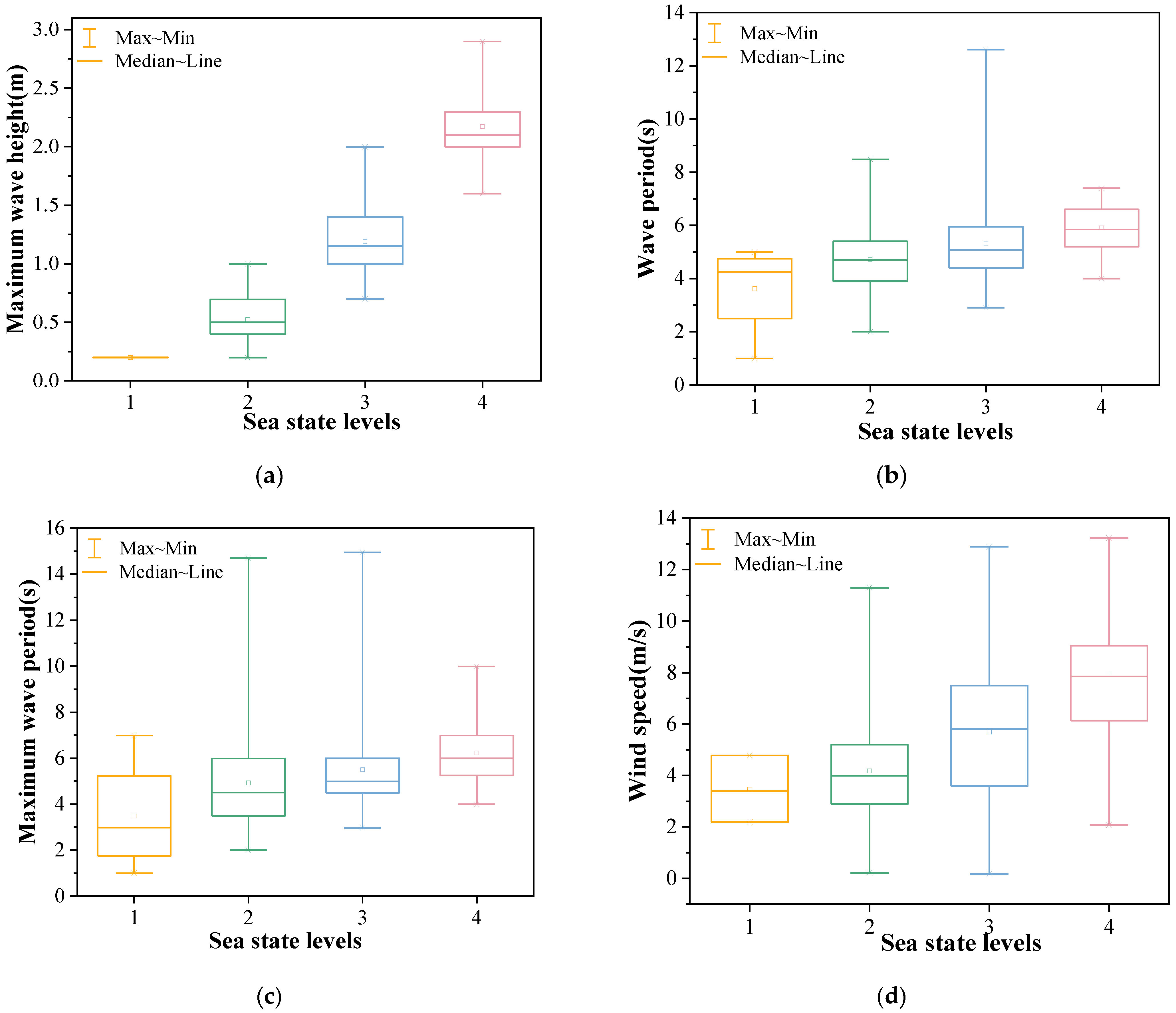
According to Table 1, it can be observed that the majority of the measured waves are from sea state 2, followed by sea state 3. Only a small portion belongs to sea state 4, and a very small fraction belongs to sea state 1. Figure 3 presents the ranges of the maximum wave height, wave period, maximum wave period, and wind speed under different sea conditions. When using the grade of wave height classification, it is evident that under the same sea state, there are significant differences in the wave period, maximum wave height, and maximum wave period, leading to variations in wave structures. Additionally, the sea surface can experience fluctuations under the influence of wind speed, affecting the fine surface structure of the sea, which, in turn, impacts electromagnetic scattering on the sea surface. Differences in wind speed under the same sea state indirectly affect wave structures. Therefore, using only significant wave height as the criterion for sea state classification is relatively crude.

To observe the spatial distribution of multiple marine environmental parameters, this study employed Principal Component Analysis (PCA) to reduce the dimensionality and visualize the multidimensional marine environmental parameters. PCA is used to transform correlated high-dimensional variables into linearly independent low-dimensional variables through orthogonal transformations. These low-dimensional variables are called principal components, which preserve the information of original data [27]. In this study, PCA was used to reduce the dataset from five dimensions to three dimensions, providing an intuitive understanding of the dataset’s overall shape. The reduced PCA components represent a linear combination of original data. By examining the weight coefficients of each principal component, we can understand the degree to which the original features contribute to each principal component. The weight coefficients of the principal components are obtained through eigenvalue decomposition of the covariance matrix.

Table 2. The weight coefficients between various components and the original marine environmental parameters.

	Component_1	Component_2	Component_3
Effective wave height (m)	0.5990	−0.0376	−0.3503
Maximum wave height (m)	0.6080	−0.0449	−0.0449
Wave period (s)	0.1934	0.7261	0.3469
Maximum wave period (s)	0.1746	0.5468	0.0763
Wind speed (m/s)	0.4511	−0.4125	0.7841

displays the weight coefficients between various components and the original marine environmental parameters.

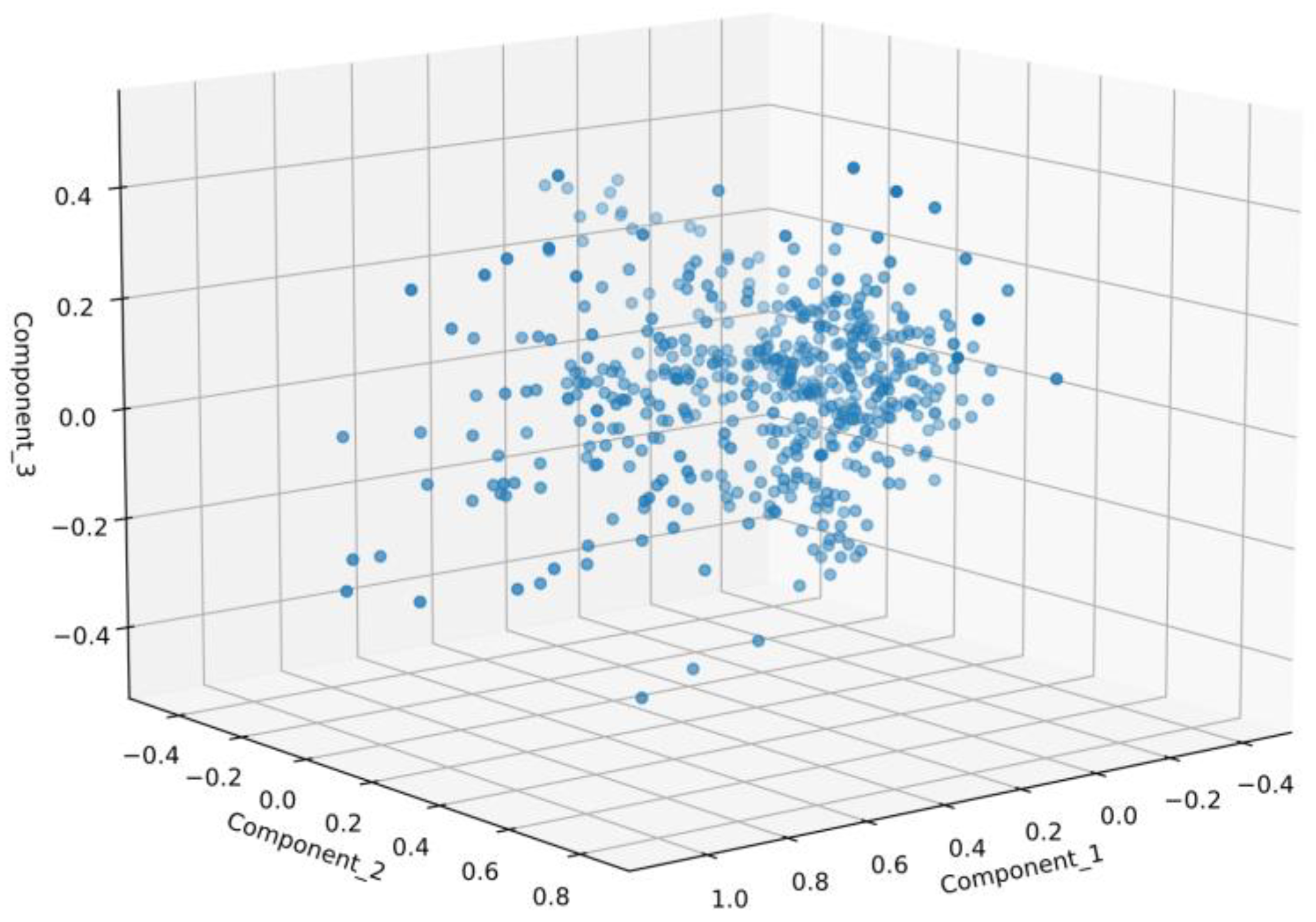
From Table 2, it can be observed that Component _1 is primarily associated with wave height and the maximum wave height, Component _2 is mainly related to the wave period, and Component _3 is predominantly linked to the wind speed. Figure 4 displays the distribution of the three main components of the reduced-dimensional marine environmental parameters in three-dimensional space.

2.1.2. Description of Sea Clutter Data

Under the same marine environment, the radar can collect sea clutter data from multiple range gates. With fixed radar parameters, the UHF radar collected a total of 516 sets of marine environmental parameters corresponding to sea clutter data. By extracting the effective region of sea clutter [13], a total of 18,476 samples of pure sea clutter data from different range gates were obtained. Figure 5 shows the variation in sea clutter reflectivity with the number of sea clutter samples.

2.2. Methods Section

In this section, the clustering algorithms used for wave structure classification, the discriminant analysis algorithm for determining wave structure categories, and the GIT-HYB-DNN model proposed in this paper for predicting sea clutter reflectivity are sequentially introduced.

2.2.1. Clustering Algorithm

Cluster analysis is a typical unsupervised learning algorithm in data mining. It can explore the inherent relationships and structures within the data and discover similar clusters within the dataset. The Affinity Propagation (AP) algorithm is a novel clustering algorithm based on exemplars [28]. The AP algorithm does not require the number of clusters or initial exemplars to be specified in advance. It only needs the similarity matrix of data points as input. By iteratively updating the availability and responsibility messages, it determines suitable exemplars.

The AP algorithm assumes initially that all samples in the dataset have an equal probability of being selected as exemplars. A similarity matrix $S$ of size $N\times N$ was constructed based on the pairwise similarity between samples. When using the Euclidean distance as the similarity metric, the similarity between any two samples $x_i$ and $x_k$ is given as follows:

$$s\left(i,k\right)=-{\parallel x_i-x_k\parallel }^2$$

(1)

where $s\left(i,k\right)$ represents the extent to which sample $x_k$ is suitable as an exemplar for sample $x_i$.

The values on the main diagonal of the matrix S are replaced with a bias parameter called preference ($p$). A higher value of $p$ indicates a higher probability of selecting that point as an exemplar. Therefore, the choice of the number of clusters in the final result may vary with different values of $p$. With the absence of prior knowledge, a common practice is to set $p$ to the median of the similarities $s\left(i,k\right)$ in the matrix S.

The AP algorithm iteratively collects evidence from the samples to select suitable exemplars. It introduces two important message parameters as follows: availability $r\left(I,k\right)$ and responsibility $a\left(I,k\right)$. The availability parameter represents the numerical message sent from sample $x_i$ to candidate exemplar $x_k$, while the responsibility parameter represents the numerical message sent from candidate exemplar $x_k$ to sample $x_i$. The availability $R\left(I,k\right)$ reflects the degree to which $x_k$ is suitable as an exemplar for $x_i$, while the responsibility $a\left(I,k\right)$ reflects the appropriateness of $x_i$ choosing $x_k$ as its exemplar. For each sample x, the sample $x_k$ with the highest sum of $r\left(I,k\right)$ and $a\left(I,k\right)$ is selected as the exemplar. The iteration process of the AP algorithm involves updating these two message parameters alternately.

The introduction of factor graphs and belief propagation theory in the AP algorithm eliminates the need to specify the number of clusters as a parameter, predefining initial cluster centers and requiring exemplar centers to correspond to actual samples in the data. These advantages make the AP clustering algorithm highly flexible and effective in practice.

2.2.2. Discriminant Analysis

Discriminant analysis is a technique used to classify samples into two or more known categories. The goal of discriminant analysis is to analyze and model the features of the samples in order to find a linear or nonlinear function that best discriminates between different categories. It achieves this by learning a discriminant function or decision boundary that maximizes the intra-class compactness and inter-class separability. Discriminant models are probabilistic approaches that model the relationship between unknown data $y$ and known data $x$. Given the input variables $x$, a discriminant model predicts $y$ by constructing a conditional probability distribution $P\left(y|x\right)$. Common discriminant models include linear regression models, linear discriminant analysis, support vector machines (SVM), neural networks, and more.

Support vector machines (SVMs) [29] are a highly effective algorithm for learning from linear or nonlinear data by minimizing structural risk to improve the ability to generalize. The Polynomial Kernel function enables SVM to map the original input features to a higher-dimensional feature space, allowing it to handle nonlinearly separable problems. By introducing the Polynomial Kernel function, SVM can learn more complex decision boundaries to accommodate more intricate data distributions.

The mathematical definition of the Polynomial Kernel function is as follows:

$$K\left(x,y\right)={\left(x·y+c\right)}^d$$

(2)

where $x$ and $y$ are input feature vectors. $c$ is a constant term and $d$ is the degree of the polynomial.

This kernel function maps the input features to a higher-dimensional feature space, where the relationships between features can be expressed via the inner product of polynomials. When $d=1$, the Polynomial Kernel function becomes a linear kernel. When $d>1$, the Polynomial Kernel function captures higher-order interactions among the input features, allowing the SVM model to learn nonlinear decision boundaries.

Compared to other kernel functions, the Polynomial Kernel function has relatively simple calculations and lower computational complexity. It is defined as the specified power, typically denoted as $d$, of the dot product of two vectors, representing the order or degree of the polynomial.

2.2.3. Sea Clutter Reflectivity Prediction Model

This paper proposes the GIT-HYB-DNN model for predicting sea clutter reflectivity by combining the following empirical models, GIT and HYB, and enhancing the DNN input parameters. This model reduces prediction errors. The empirical models are derived from summarized and measured data and are used to estimate the sea clutter amplitude mean. By inputting certain marine environmental parameters, this model provides the sea clutter amplitude mean for that specific condition. The GIT model [3], proposed by the Georgia Institute of Technology in the 1970s, is a backscattering reflectivity model based on measured data and mathematical models of different sea surface scattering mechanisms. Its notable feature is the simultaneous use of wind speed and significant wave height to describe the sea conditions. The HYB model [5] is a modification of the GIT model, consisting of a reference reflectivity and four correction terms. It provides estimates of average sea clutter backscattering reflectivity across all frequency ranges. The reflectivity is represented by ${\sigma }^0$ and is expressed in decibels (dB).

The expression of the GIT model is as follows:

$${\sigma }_{GIT}^0=10\left({\log }_{10}(\lambda {\varphi }_{\mathrm{g}\mathrm{r}}^{0.4}{A}_i{A}_u{A}_w\right)-54.09)$$

(3)

$$A_i=\frac{{\sigma }_{\varphi }^4}{1+{\sigma }_{\varphi }^4}$$

(4)

$${\sigma }_{\varphi }=({\varphi }_{\mathrm{g}\mathrm{r}}{SS}^2\left(1.152\lambda +0.44\right))/\lambda$$

(5)

$$A_u=\exp \left[0.2\left(1-2.8{\varphi }_{\mathrm{g}\mathrm{r}}\right)\cos \left({\theta }_w\right){\left(\lambda +0.015\right)}^{-0.4}\right]$$

(6)

$$A_w={\left(\frac{1.95U}{1+\frac{U}{15.4}}\right)}^{\frac{1.1}{{\left(\lambda +0.015\right)}^{0.4}}}$$

(7)

The specific calculation expression of the HYB model is as follows:

$${\sigma }_{HYB}^0=-77.96-24.4{\log }_{10}\left(\lambda \right)+K_{\mathrm{g}}+K_s+K_p+K_d$$

(8)

$$K_{\mathrm{g}}=\left\{\begin{array}{l} 20{\log }_{10}\left(\frac{{\varphi }_{\mathrm{g}\mathrm{r}}}{{\varphi }_{\mathrm{r}\mathrm{e}\mathrm{f}}}\right), 0.0017={\varphi }_{\mathrm{r}\mathrm{e}\mathrm{f}}\le {\varphi }_{\mathrm{g}\mathrm{r}}\le {\varphi }_{\mathrm{t}}={\sin }^{-1}\left(\frac{0.0894\lambda }{SS}\right)\\ 20{\log }_{10}\left(\frac{\sqrt{{\varphi }_{\mathrm{g}\mathrm{r}}{\varphi }_{\mathrm{t}}}}{{\varphi }_{\mathrm{r}\mathrm{e}\mathrm{f}}}\right), {\varphi }_{\mathrm{t}}<{\varphi }_{\mathrm{g}\mathrm{r}}\le \pi /6\end{array}\right.$$

(9)

$$K_s=5\left(SS-5\right)$$

(10)

$$K_p=\ln \left(\frac{{\left(0.08{SS}^2+0.015\right)}^{1.7}}{{\lambda }^{3.7}{\left(0.0001+{\varphi }_{\mathrm{g}\mathrm{r}}\right)}^{2.5}}\right)-22.2$$

(11)

$$K_d=\left(2+1.7{\log }_{10}\left(0.1/\lambda \right)\right)\left(\cos {\theta }_w-1\right)$$

(12)

where $\lambda$ represents the radar wavelength, ${\varphi }_{\mathrm{g}\mathrm{r}}$ represents the ground wiping angle, U represents the wind speed, SS represents the sea state, and ${\theta }_w$ represents the wind direction angle. ${\sigma }_{\varphi }$ is the roughness parameter, which is an input for the interference factor $A_i$. $A_i$ represents the interference factor in the GIT model. $A_u$ represents the wind direction factor in the GIT model, while $A_w$ represents the wind speed factor in the GIT model. $K_{\mathrm{g}}$, $K_s$, $K_p$, and $K_d$ are the correction factors relative to the grazing angle, sea state, polarization, and wind direction.

Based on the marine environmental parameters and sea clutter reflectivity database, a deep neural network (DNN) was used to establish a high-order, multi-dimensional, nonlinear mapping model between sea clutter characteristics and marine environmental parameters in the Yellow Sea region. The GIT-HYB-DNN prediction model is primarily responsible for data transformation between various sea clutter characteristics and marine environmental elements, including the input layer, multiple fully connected layers, and the output layer. Each layer builds upon the expression of the previous layer, seeking the correlation between marine environmental parameters and sea clutter characteristics in high-dimensional space, with the output being the sea clutter reflectivity. The structure of the GIT-HYB-DNN model is illustrated in Figure 6.

In Figure 6, the activation function chosen for the two adjacent hidden layers is the rectified linear unit (ReLU). The loss function used is the root mean square error (RMSE), which calculates the square root of the ratio of the squared deviations between the predicted and true values to the number of observations (n). It measures the deviation between the predicted and true values and is sensitive to outliers in the data. The model parameters are trained using the Adaptive Moment Estimation (Adam) algorithm, which is an adaptive optimization algorithm commonly used for training neural networks. Adam combines the advantages of adaptive gradient adjustment and momentum methods and is widely applied in deep learning.

The input data included 5 marine environmental parameters used for wave structure classification, as well as wave direction and wind direction. Additionally, there were functions related to the grazing angle in the GIT and HYB models, the wind direction factor and interference factor in the GIT model, the grazing angle correction factor and polarization correction factor in the HYB model, and computational parameters (sea state and grazing angle), as shown in

Table 3. GIT-HYB-DNN model input parameters.

Parameter Source	Name	Symbol
Sea Wave Parameters	Significant wave height	$H_s$
	Maximum wave height	$H_{max}$
	Wave direction	$\varphi$
	Wave period	$T$
	Maximum wave period	$T_{max}$
Wind Parameters	Wind speed	U
	Wind direction	$\phi$
Calculating Parameters	Sea state	$SS$
	Grazing angle	${\varphi }_{\mathrm{g}\mathrm{r}}$
GIT Model Parameters	Interference factor	$A_i$
	Wind factor	$A_u$
HYB Model Parameters	Correction factor for grazing Angle	$K_{\mathrm{g}}$
	Correction factor for polarization	$K_p$

.

3. Results

3.1. Wave Structure Clustering Results and Analysis

3.1.1. Clustering Results

We performed Affinity Propagation (AP) clustering analysis on 516 sets of measured marine environmental parameter data. Following the research findings in reference [30], the IGP is selected as the clustering validity index, and cross-validation was employed to determine suitable hyperparameter values. The optimal hyperparameter values yielded six clusters as the result of AP clustering.

Table 4. The number and proportion of marine environment parameter sets in each category after clustering marine environment parameter.

Category Names (Class Number)	Calm (1)	Visible (2)	Small (3)	Gentle (4)	Smooth (5)	Moderate (6)
Number of marine environment parameter sets	121	39	123	99	81	53
Percentage	23.4%	7.6%	23.8%	19.2%	15.7%	10.3%

provides the quantity of each cluster obtained from the AP clustering.

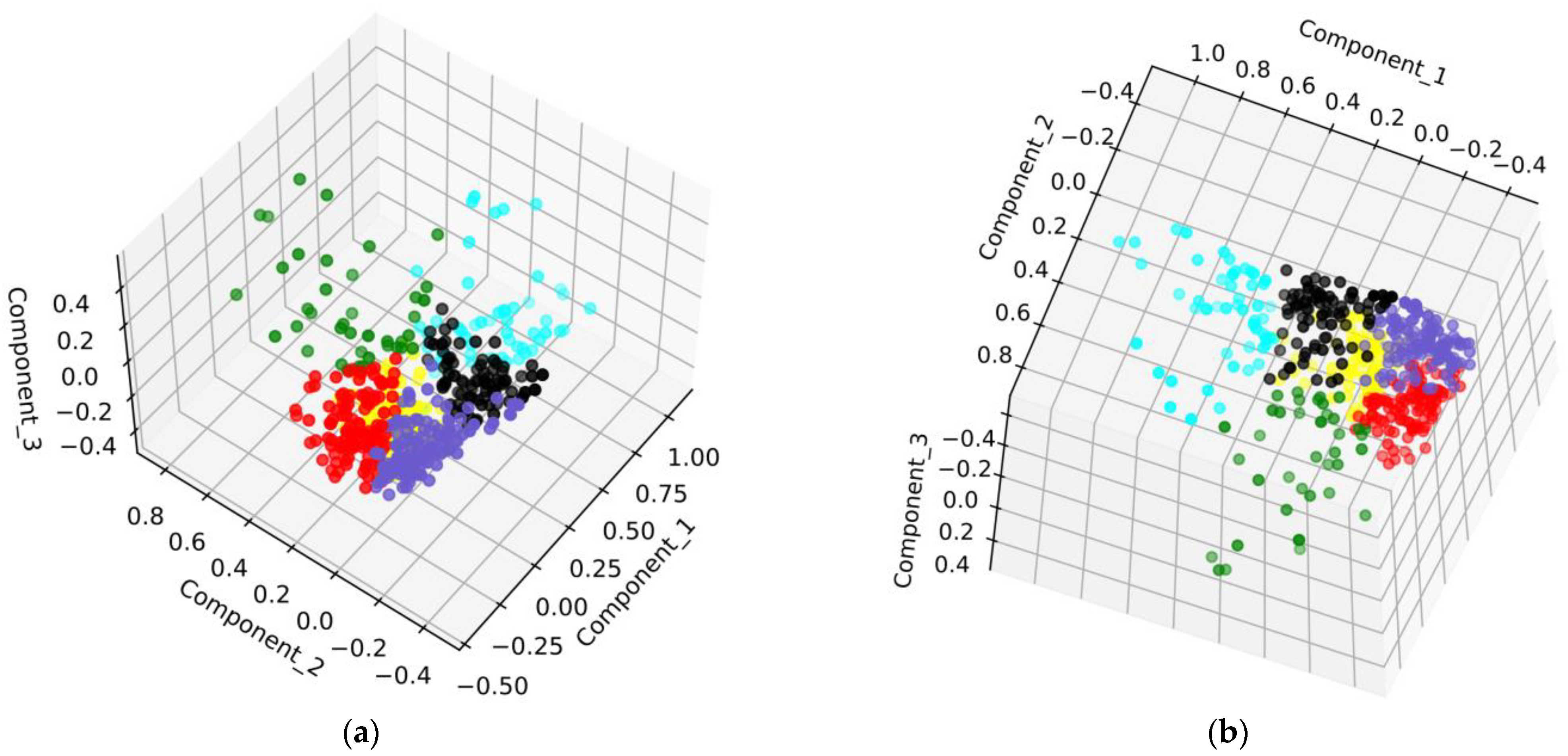
According to Table 4, a small portion of the data formed a separate cluster, while the remaining data were relatively and evenly distributed among other clusters. To visualize the clustering results effectively, PCA was applied to reduce the dimensionality of the data. The resulting three-dimensional visualization is shown in Figure 7, where each color represents a different cluster. The clustering results are displayed from two different perspectives. It can be observed that the AP clustering yielded favorable results, with clear boundaries between different clusters. Figure 7a shows that this particular category represented using green dots, exhibits significant differences in the direction of Component_2 compared to other categories. From Figure 7b, it can be observed that the boundaries of each category become distinct as Component_1 increases.

3.1.2. Analysis of Wave Structure Clustering Results

Based on the clustering results of marine environmental parameters, an analysis was conducted on significant wave height, maximum wave height, wave direction, wave period, maximum wave period, wind speed, wind direction, and the grazing angle in different wave structures. These marine environmental parameters also served as input data for the training predictive models of sea clutter reflectivity corresponding to different wave structures.

Table 5. The range of different marine environmental parameters in different wave structures.

Class	1	2	3	4	5	6
Significant wave height (m)	0.1~0.45	0.2~1	0.1~0.7	0.4~1.1	0.5~1.19	0.8~1.9
Maximum wave height (m)	0.15~0.8	0.2~1.5	0.2~1.1	0.6~1.6	0.79~1.89	1.2~2.9
Wave direction (°)	8.24~309.95	7.69~346.26	8.18~358.68	13.75~147.45	11.27~167.89	6.3~144.52
Maximum wave period (s)	3~7.99	6.5~15.93	2.45~6.48	2.52~7.24	2.48~6.98	4.5~11
Wave period (s)	3.19~7.24	5.2~12.16	2.6~5.3	3.9~7.2	2.79~6.74	4.6~7.6
Wind speed (m/s)	0.21~6.99	1.14~10.49	1.39~10.7	0.18~5.18	4.69~11.8	0.69~13.67
Wind direction (°)	0.25~358.92	0.39~357.7	0.24~358.88	0.98~359.53	0.39~359.5	0.98~359.5

provides the ranges of marine environmental parameters for six categories of wave structures.

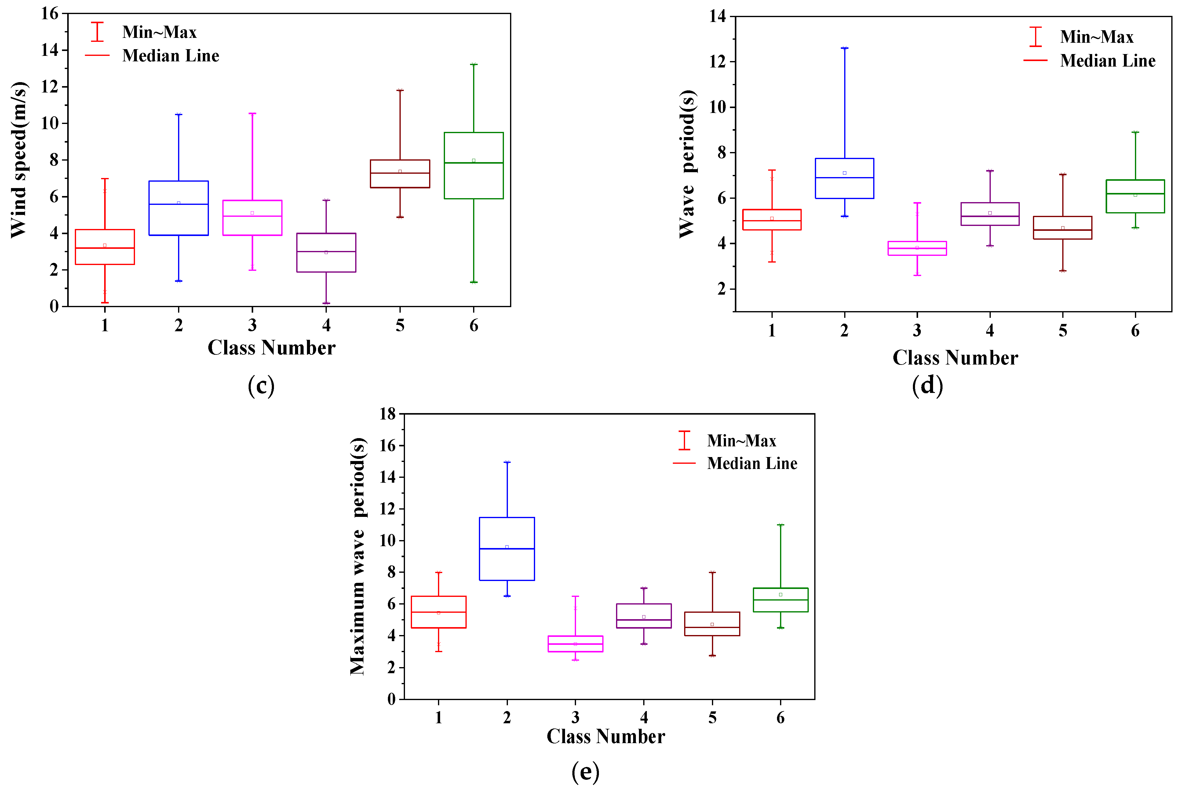
Figure 8 presents the ranges of marine environmental parameters for the six identified wave structures. From Figure 8, it can be observed that significant wave height, maximum wave height, wave period, and maximum wave period had a significant impact on wave structures, while wind speed, as an indirect factor, did not have a clear direct influence on wave structures, aligning with the objective reality. Among these six wave structures, except for the second class, there were notable differences in wave height and maximum wave height between each class, indicating distinct variations in the peak positions of the wave structures. The second wave structure exhibits wave heights within the range of the third and fourth classes but has the overall maximum wave period. Under the same wave speed, a larger wave period corresponded to a longer wavelength, suggesting a higher probability of this wave structure being a swell.

3.2. Construction of Discriminant Model

In order to determine the category of newly collected marine environmental parameters, this study constructs a discriminant model based on clustering. The 516 sets of clustered marine environmental data are labeled with categories ranging from 1 to 6. Out of these, 482 sets were randomly selected as the training and test sets, while 32 sets served as the validation set for training the discriminant model. The training set and test set were in a ratio of 8:2, and the resulting discriminant model achieved an accuracy of 96%. After evaluating the 32 samples in the validation set, 30 of them were correctly classified, and 2 were misclassified, resulting in a validation accuracy of 94%. The high accuracy of this discriminant model allowed it to be used for determining the categories of new marine environmental parameter data. By inputting marine environmental parameters into the corresponding sea clutter reflectivity prediction model, sea clutter reflectivity could be obtained.

3.3. Sea Clutter Reflectivity Prediction Results

This section is divided into two parts. In the first part, without clustering marine environmental parameters or wave structure classification, the training and test sets are divided based on all measured data. The GIT-HYB-DNN model was trained and used to predict sea clutter reflectivity. In the second part, after clustering the marine environmental parameters, a separate GIT-HYB-DNN model is established for each wave structure category to predict the sea clutter reflectivity.

3.3.1. Sea Clutter Reflectivity Prediction Results without Clustering of Marine Environmental Parameters

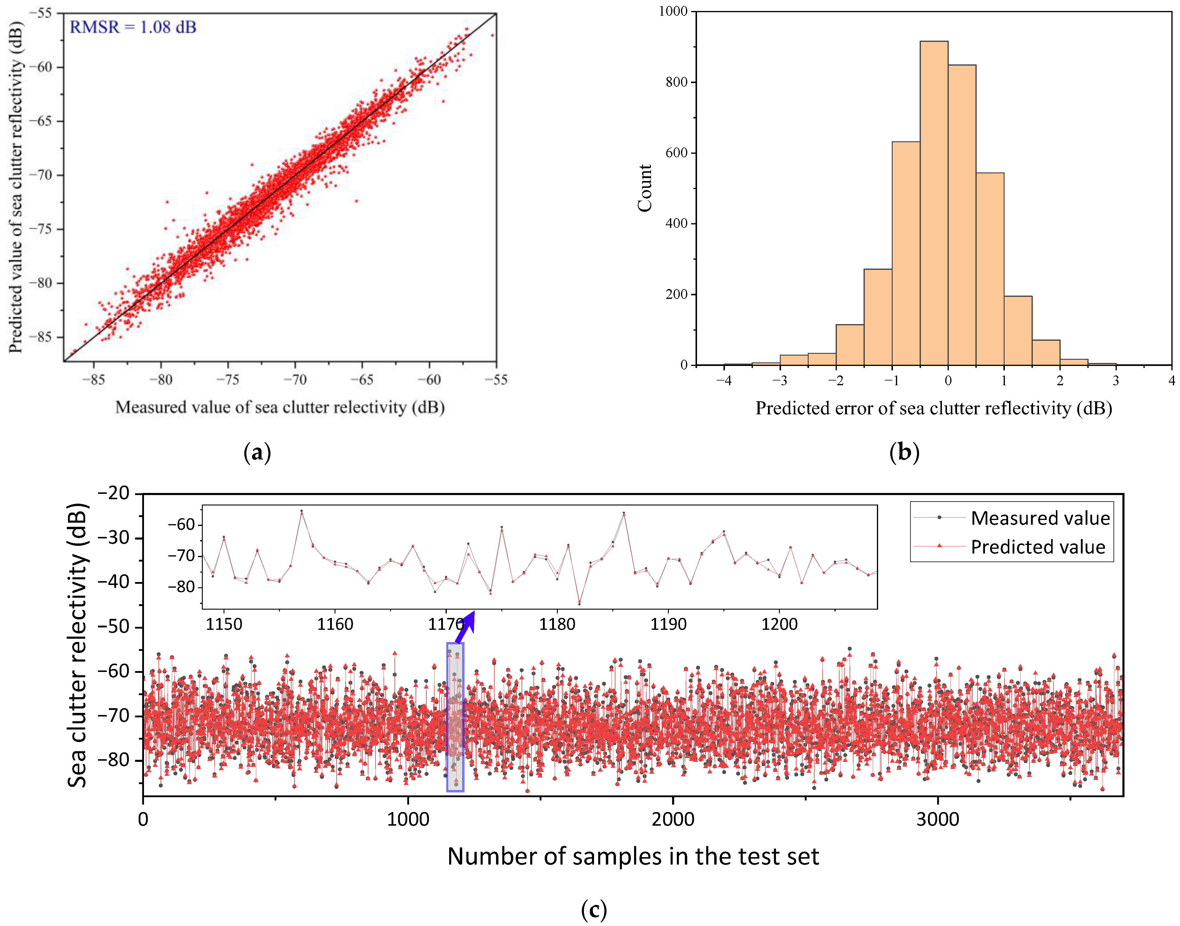
Under the same marine environmental conditions, the radar can collect sea clutter data from multiple range gates. After extracting effective sea clutter data, there were a total of 18,476 samples of sea clutter data corresponding to different range gates from the 516 sets of marine environmental parameters. Based on the GIT-HYB-DNN model proposed in this paper, all 18,476 measured data samples were used for sea clutter reflectivity prediction. The data were randomly divided into training, validation, and test sets with proportions of 64%, 16%, and 20%, respectively. The neural network was trained, and parameters were adjusted to achieve the minimum root mean square error (RMSE) on the test set, which was 1.08 dB. Under the same experimental data conditions, this RMSE was higher in accuracy compared to the prediction results of the NRL-MSINN model (1.23 dB) [31]. The test set prediction results are shown in Figure 9. Figure 9a displays a comparison between the measured sea clutter reflectivity and predicted reflectivity. The x-axis represents the measured reflectivity values obtained via calculating sea clutter time series based on the radar equation, while the y-axis represents the predicted reflectivity values. Figure 9b shows the histogram of the differences between the measured reflectivity values and the predicted reflectivity values. Figure 9c shows the line plot of measured and predicted values of reflectivity, and a random part was selected for amplification.

It can be observed that the true and predicted values are very close to the y = x line, and the prediction errors were mainly concentrated within the range of −1 dB to 1 dB. In the line plot, the measured values of reflectivity are close to the predicted values.

3.3.2. Sea Clutter Reflectivity Prediction Results Based on Classification of Wave Structures

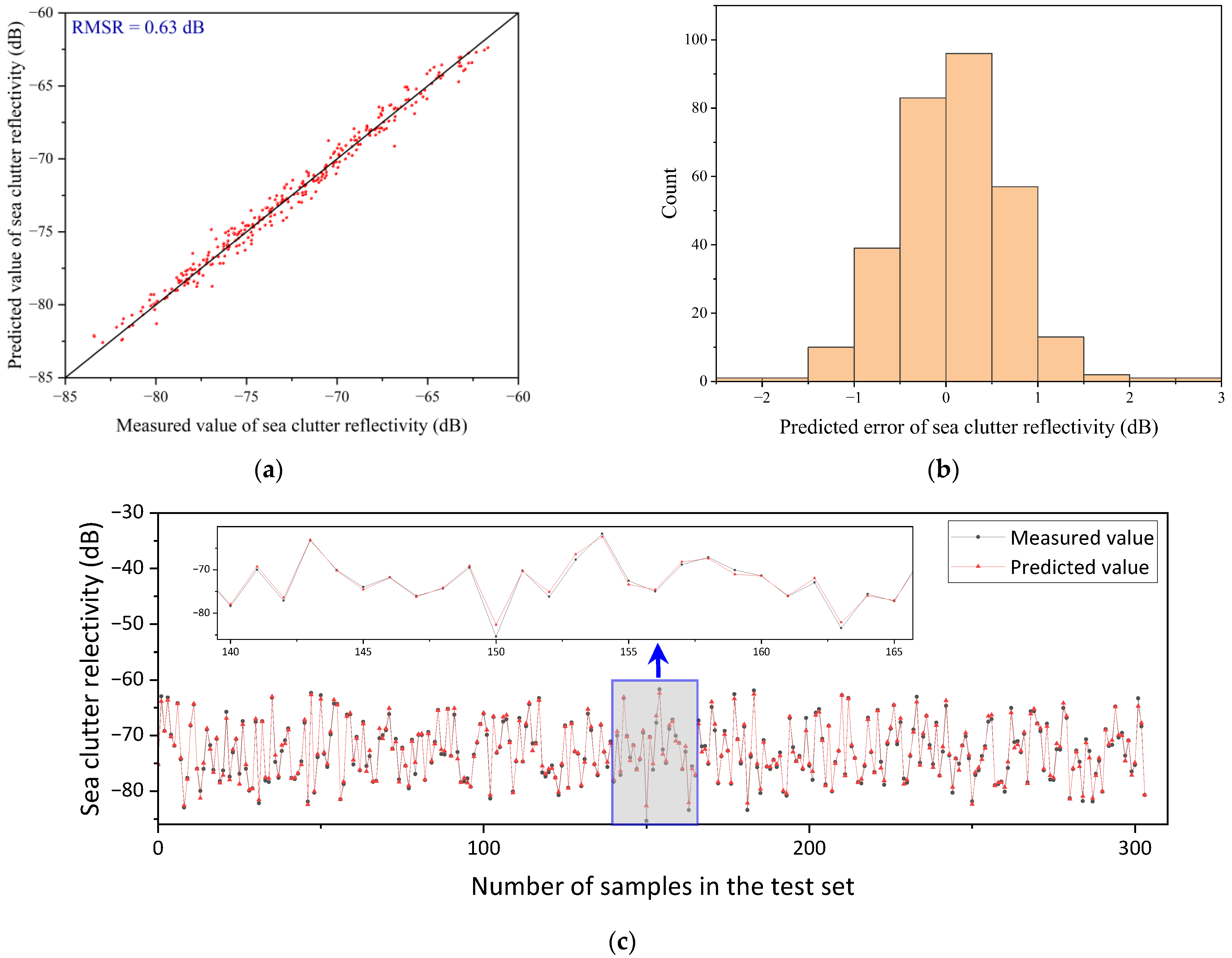
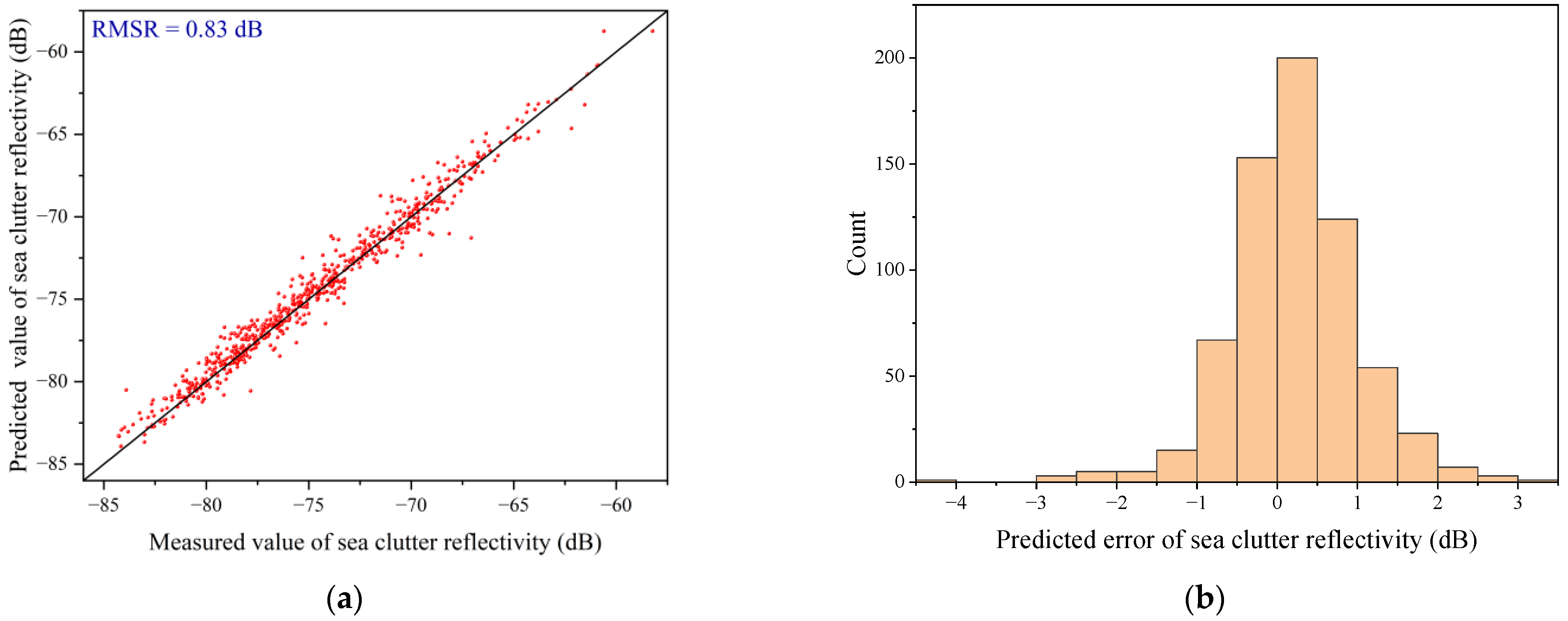
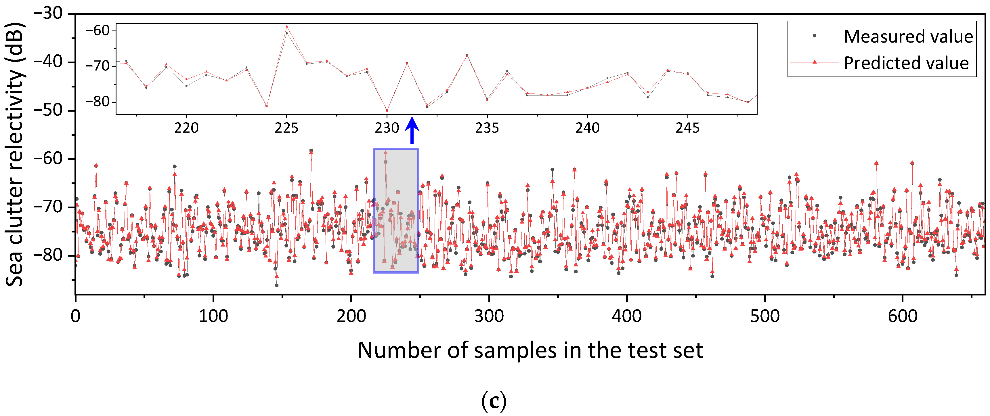
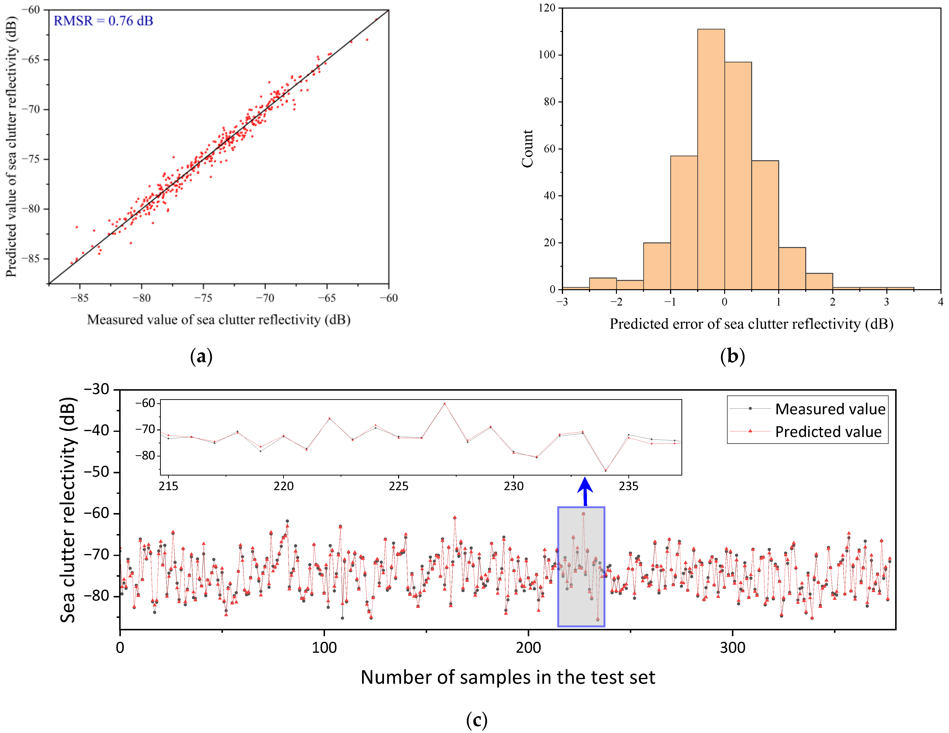
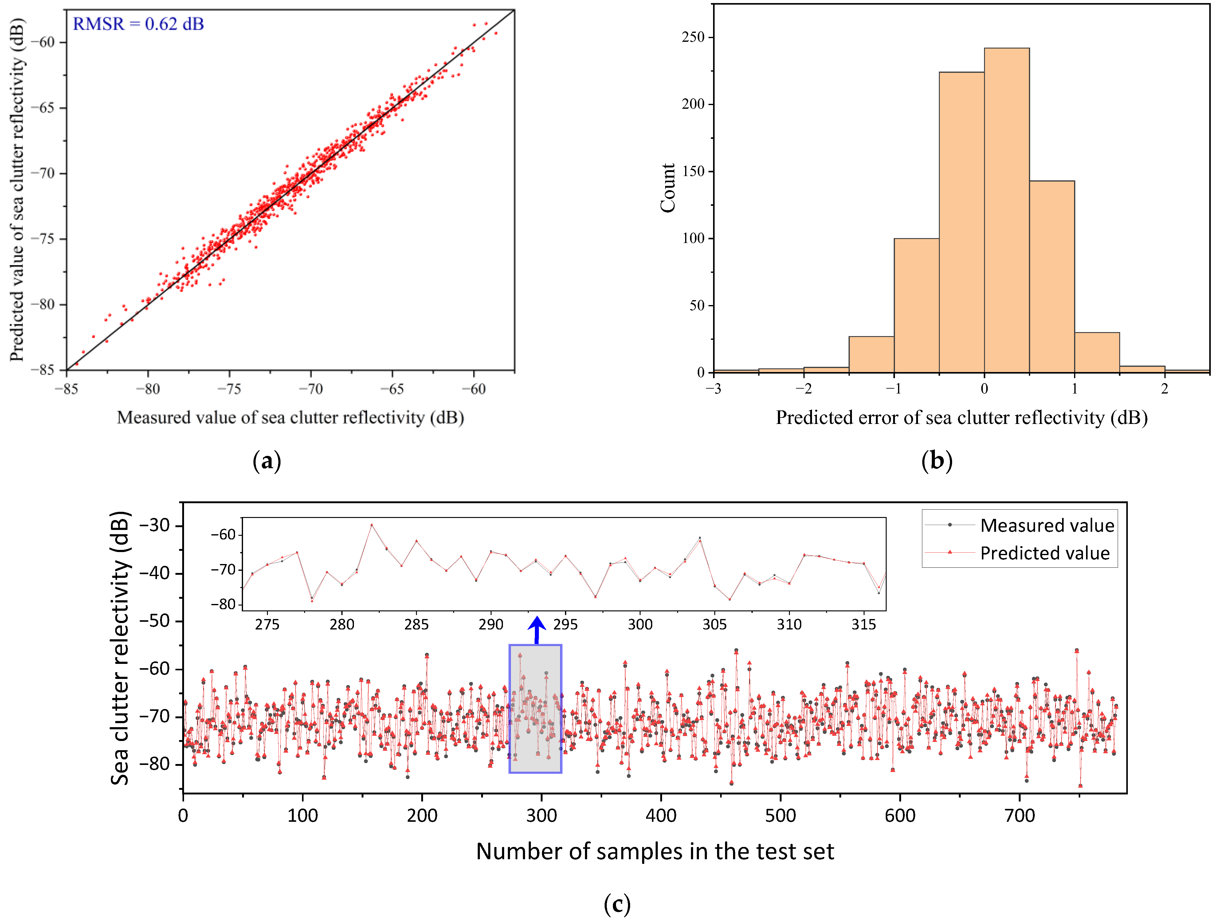
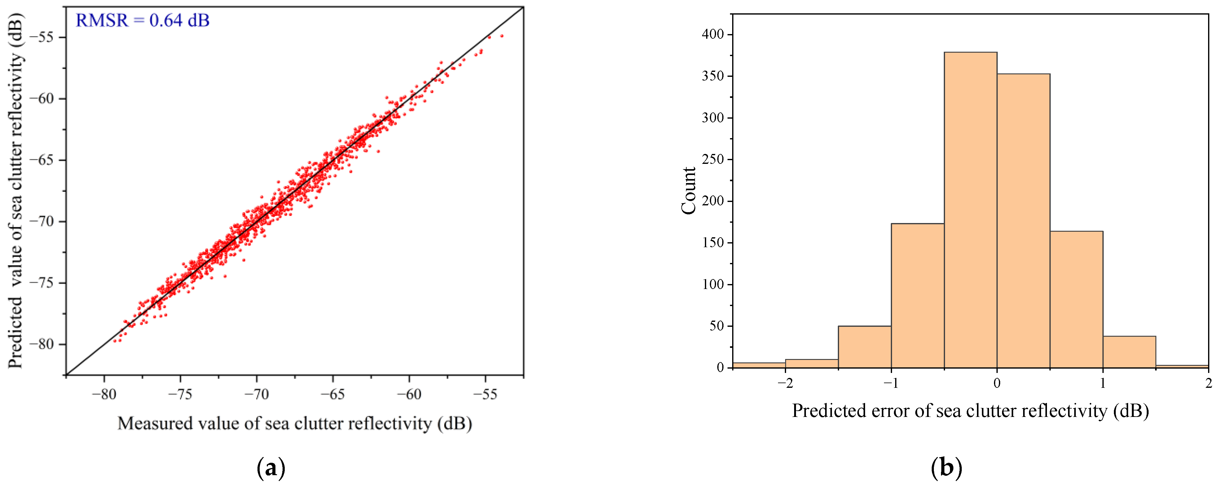
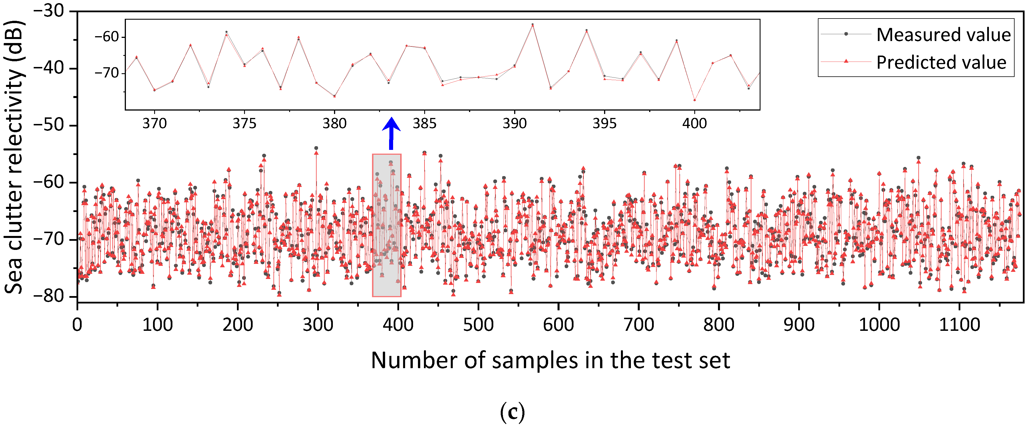
For each of the six categories of wave structures, this study conducted separate training and testing of the sea clutter reflectivity prediction models (GIT-HYB-DNN). The number of sea clutter data for each category was 1954, 1524, 3309, 1893, 3915, and 5881, respectively. The data were divided into training sets (64%), validation sets (16%), and testing sets (20%). After training the GIT-HYB-DNN models for each wave structure category, the minimum root mean square errors (RMSEs) for the testing sets were found to be 0.84 dB, 0.63 dB, 0.83 dB, 0.76 dB, 0.62 dB, and 0.64 dB, corresponding to the 1st to 6th wave structure categories, respectively. Figure 10, Figure 11, Figure 12, Figure 13, Figure 14 and Figure 15 depict the sea clutter reflectivity prediction results for the corresponding 1st to 6th wave structure categories. Figure 10a, Figure 11a, Figure 12a, Figure 13a, Figure 14a and Figure 15a display scatter plots of true reflectivity values against predicted reflectivity values. The x-axis represents the true reflectivity values obtained through radar equation calculations of the sea clutter sequences, and the y-axis represents the predicted reflectivity values. Figure 10b, Figure 11b, Figure 12b, Figure 13b, Figure 14b and Figure 15b present histograms of the differences between true and predicted reflectivity values. Figure 10c, Figure 11c, Figure 12c, Figure 13c, Figure 14c and Figure 15c are line plots of measured and predicted values of reflectivity, and a random part was selected for amplification.

The RMSE of the predicted sea clutter reflectivity models for the six categories of wave structures ranged from 0.62 dB to 0.84 dB. In the line plot, the measured values of reflectivity are very close to the predicted values. The prediction errors for classes 2 to 6 are primarily concentrated within the range of −0.5 to 0.5 dB, while class 1 is mainly concentrated within the range of −1 to 1 dB. Within classes 1 and 3, only a few prediction errors exceed 3 dB, while the remaining prediction errors are within 3 dB. Overall, through marine environmental clustering and fine classification of wave structures, the sea clutter reflectivity prediction performance improved for each specific wave structure category.

4. Discussion

This section includes the selection of the dataset division ratio to establish the discriminative model and a comparison of methods for improving the predictive performance of sea clutter reflectivity. This study mainly improves the predictive performance of sea clutter reflectivity through two aspects. Firstly, it finely divides the wave structures using a clustering algorithm, which is an unsupervised learning method. This algorithm divides the marine environmental parameter data into six different clusters based on similarity. Waves within the same cluster have similar structures, leading to similar scattering characteristics. Secondly, it utilizes a high-precision prediction model called GIT-HYB-DNN, whose inputs include various marine environmental parameters, considering more comprehensive influencing factors. It combines the rational elements from the empirical models GIT and HYB with the learning ability of deep neural networks. By combining these two methods, different prediction models are established for each type of wave structure. The input data for each model have high similarity and strong internal correlation, resulting in a reduction in sea clutter reflectivity prediction error in the Yellow Sea region range from 0.62 to 0.84 dB.

4.1. Division of Training Set and Test Set for Discriminant Model

When constructing the discriminant model, the 516 groups of labeled marine environmental data were divided into training and test sets using four different partition ratios as follows: 6:4, 7:3, 8:2, and 9:1. Training was performed separately for each ratio, and

Table 6. The accuracy of the discriminant model under different dataset divisions.

Ratio of Training Set to Test Set	16:4	7:3	8:2	9:1
Accuracy rate (%)	77	86	94	88

presents the accuracy of the discriminant model under different dataset divisions. Based on Table 6, it is evident that the accuracy was highest when the training-to-testing dataset split ratio was 8:2.

4.2. Sea Clutter Reflectivity Prediction

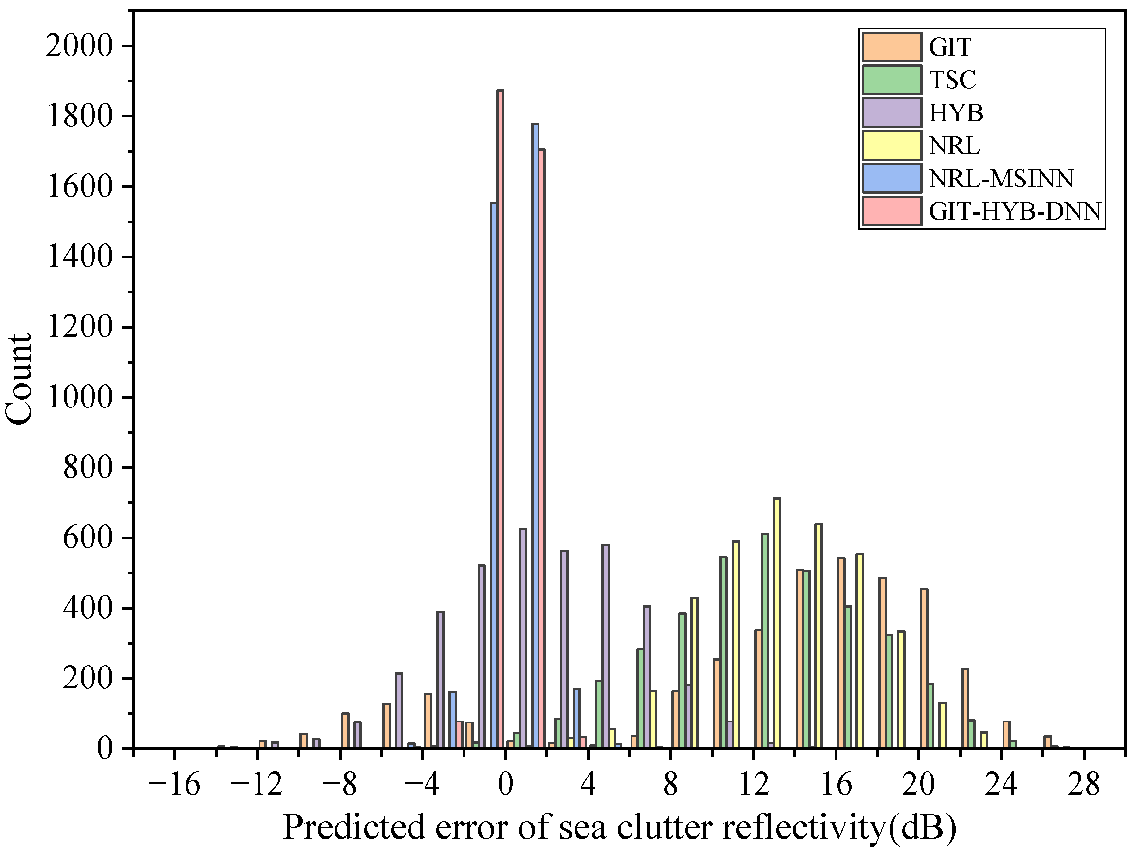
Based on the test data in Figure 9, we compared the predictive performance of four empirical models, the NRL-MSINN model and our GIT-HYB-DNN model. Figure 16 displays the distribution of the differences between the predicted sea clutter reflectivity and the true values for each method. The bin size is 2 dB. It can be observed that the GIT model’s prediction errors were mainly distributed in the range of 12 to 20 dB and were relatively scattered, with fewer instances near the 0-dB line. The TSC and NRL models have similar error distributions, approximately following a normal distribution, and are mainly concentrated in the range of 10 to 18 dB. The HYB model’s prediction errors are primarily distributed in the range of −2 to 6 dB. Both the GIT-HYB-DNN model and the NRL-MSINN model have prediction errors concentrated around the 0-dB line, with the GIT-HYB-DNN model showing a more centralized distribution.

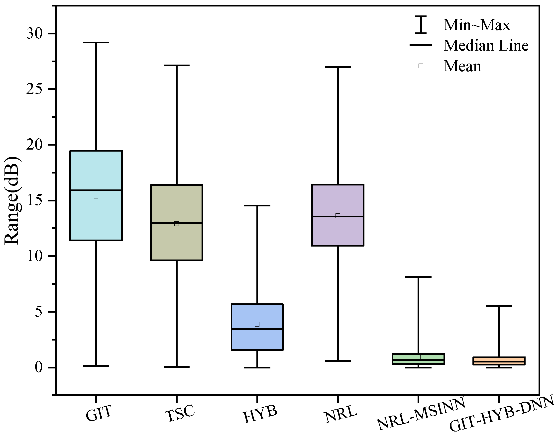
Figure 17 illustrates the absolute value distribution of the differences between the true values and the predicted values for each method. It can be observed that the median and mean of the prediction errors for the GIT, TSC, and NRL models are around 15 dB. Among the four empirical models, the HYB model demonstrates the best predictive performance. However, the NRL-MSINN model and the GIT-HYB-DNN model exhibit lower mean and median prediction errors, with the GIT-HYB-DNN model having the lowest values.

In Figure 18, a comparison is made between the prediction error distributions of the NRL-MSINN model and the GIT-HYB-DNN model, with a bin size of 1 dB. It can be observed that the GIT-HYB-DNN model had a higher frequency of occurrences in the range of −1 to 1 dB and fewer occurrences in other bin ranges. This indicates that the GIT-HYB-DNN model has smaller prediction errors and higher accuracy. Therefore, the GIT-HYB-DNN model demonstrates superior predictive performance compared to the NRL-MSINN model.

4.3. Prediction of Sea Clutter Reflectivity for Different Wave Structures

By clustering five sea environmental parameters in the Yellow Sea region, namely significant wave height, maximum wave height, wave period, maximum wave period, and wind speed, the waves were divided into six different structures. For each of the six wave structures, sea clutter reflectivity was predicted using the NRL-MSINN model and the GIT-HYB-DNN model.

Table 7. RMSE results predicted using the NRL-MSINN and GIT-HYB-DNN models for various wave structures.

Class	1	2	3	4	5	6
RMSE of the NRL-MSINN model (dB)	0.98	0.73	0.98	0.88	0.76	0.77
RMSE of the GIT-HYB-DNN model (dB)	0.84	0.63	0.83	0.76	0.62	0.64

presents the root mean square error (RMSE) results for the predictions of sea clutter reflectivity using the NRL-MSINN model and the GIT-HYB-DNN model for each of the six wave structures. It can be observed that the RMSE obtained from NRL-MSINN model predictions ranged from 0.73 to 0.98 dB, showing an improvement in predictive accuracy compared to the non-divided case with a prediction accuracy of 1.23 dB [31]. The RMSE from the GIT-HYB-DNN model predictions ranged from 0.62 to 0.84 dB, also indicating an improvement in predictive accuracy compared to the non-divided case with a prediction accuracy of 1.08 dB. Both models showed an increase in sea clutter reflectivity prediction accuracy, suggesting that the fine division of wave structures led to the improved predictive accuracy of sea clutter reflectivity.

4.4. Limitations of This Study and Directions for Future Research

The data in this paper were collected in the Yellow Sea region over a certain period, where the marine environment was complex and constantly changing. This study only considers data for the grade of wave height sea state levels 1 to 4. In order to comprehensively model sea clutter reflectivity prediction, it is necessary to include data from more sea states. The application of the AP clustering algorithm in this study resulted in a refined classification of wave structures into six categories. With a larger dataset, it is possible to achieve an even more detailed classification of wave structures.

In future research, there is a need to expand the dataset, especially by collecting data from a wider range of marine areas and over a longer time span, to obtain a more comprehensive and diverse set of marine environmental samples, thus enhancing the model’s generalization ability and predictive accuracy. It is also worth considering the use of deep clustering algorithms to explore wave structures further. This paper focuses solely on the sea clutter reflectivity; however, adopting the concept of refined wave structure, it is possible to investigate other characteristics of sea clutter.

5. Conclusions

This study improves the prediction accuracy of sea clutter reflectivity in the Yellow Sea by clustering multiple marine environmental parameters. It also proposes a refined classification criterion for wave structures based on significant wave height, maximum wave height, wave period, maximum wave period, and wind speed, along with the establishment of a discrimination model. Additionally, the scattering characteristics of sea clutter are investigated using deep neural networks, providing technical support for radar system parameter selection and sensing platforms in maritime environments.

For future research, it is recommended that a wider range of marine environmental parameters be analyzed using more suitable clustering methods to achieve a higher prediction accuracy. Furthermore, the research approach presented in this study can be applied to other marine areas, enabling the high-precision prediction of sea clutter reflectivity in multiple regions.

References

1. Wen, B.; Wei, Y.; Lu, Z. Sea Clutter Suppression and Target Detection Algorithm of Marine Radar Image Sequence Based on Spatio-Temporal Domain Joint Filtering. Entropy 2022, 24, 250. [Google Scholar] [CrossRef] [PubMed]
2. Nuoyi, Z.; Yeesock, K.; Kyu-Han, K.; Bum-Shick, S. Change detection of ocean wave characteristics. Expert Syst. Appl. 2016, 51, 245–258. [Google Scholar] [CrossRef]
3. Ewell, G.; Horst, M.; Tuley, M. Predicting the Performance of Low-Angle Microwave Search Radars—Targets, Sea Clutter, and the Detection Process. In Proceedings of the OCEANS ‘79, San Diego, CA, USA, 17–19 September 1979; pp. 373–378. [Google Scholar]
4. Antipov, I. Simulation of Sea Clutter Returns; Defence Science and Technology Organisation Canberra (Australia): DSTO-TR-0679; Defense Technical Information Center: Fort Belvoir, VA, USA, 1998.
5. Reilly, J.; Dockery, G. Influence of evaporation ducts on radar sea return. IEE Proc. F (Radar Signal Process.) 1990, 137, 80–88. [Google Scholar]
6. Gregers-Hansen, V.; Mital, R. An Improved Empirical Model for Radar Sea Clutter Reflectivity. IEEE Trans. Aerosp. Electron. Syst. 2012, 48, 3512–3524. [Google Scholar] [CrossRef]
7. Rosenberg, L.; Watts, S. Continuous sea clutter models for the mean backscatter and K-distribution shape. In Proceedings of the International Conference on Radar Systems (Radar 2017), Belfast, Ireland, 23–26 October 2017; pp. 1–6. [Google Scholar]
8. Watts, S.; Rosenberg, L. Challenges in radar sea clutter modelling. IET Radar Sonar Nav. 2022, 16, 1403–1414. [Google Scholar] [CrossRef]
9. Zhang, Y.; Zhang, J.; Li, X.; Wu, Z. Modified GIT model for predicting wind-speed behavior of low-grazing-angle radar sea clutter. Chin. Phys. B 2014, 23, 108402. [Google Scholar] [CrossRef]
10. Wu, G.; Fan, J.; Zhang, F.; Lu, F. A Semi-Empirical Model of Sea Clutter Based on Zero Memory Nonlinearity. IEEE Access 2019, 7, 18125–18137. [Google Scholar] [CrossRef]
11. Chen, P.; Jia, Z.; Su, Q.; Fan, Q. Sea clutter reflection coefficient model and radar echo signal calculation method. Mod. Def. Technol. 2020, 48, 81–85. [Google Scholar]
12. Li, X.; Xia, X.; Zhang, Y.; Shui, P.L.; Zhang, J. Modified reflectivity model of UHF-band sea clutter at low grazing angle. J. Syst. Eng. Electron. 2020, 42, 1035–1040. [Google Scholar]
13. Ma, L.; Wu, J.; Zhang, J.; Wu, Z.; Jeon, G.; Zhang, Y.; Wu, T. Research on Sea Clutter Reflectivity Using Deep Learning Model in Industry 4.0. IEEE. Ind. Inform. 2020, 16, 5929–5937. [Google Scholar] [CrossRef]
14. Shi, X.F. Research on Prediction Method of Key Characteristic Parameters of Sea Clutter. Master’s Thesis, Xidian University, Xi’an, China, 2020. [Google Scholar]
15. Shui, P.L.; Shi, X.F.; Li, X.; Feng, T.; Xia, X.Y.; Han, Y. GRNN-Based Predictors of UHF-Band Sea Clutter Reflectivity at Low Grazing Angle. IEEE Geosci. Remote Sens. Lett. 2022, 19, 1–5. [Google Scholar] [CrossRef]
16. Wang, C. A High-Precision Calculation Method for the Average Backscatter Coefficient of Sea Clutter under High Sea Conditions. Chinese Patent CN115984505A, 18 April 2023. [Google Scholar]
17. GB/T 42176-2022; The Grade of Wave Height. Standardization Administration of China: Beijing, China, 2023.
18. Liu, N.; Jiang, X.; Ding, H.; Xu, Y.; Guan, J. Wave Height Inversion and Sea State Classification Based on Deep Learning of Radar Sea Clutter Data. In Proceedings of the 2021 International Conference on Control, Automation and Information Sciences, Xi’an, China, 14–17 October 2021; pp. 34–39. [Google Scholar]
19. Das, N.; Hossain, M.S. Investigation of the Impact of Sea Conditions on the Sea Surface Reflectivity in Maritime Radar Sea Clutter Modeling. In Proceedings of the 2023 International Conference on Electrical, Computer and Communication Engineering, Chittagong, Bangladesh, 23–25 February 2023; pp. 1–4. [Google Scholar]
20. Yang, B.; Jiang, M.; Wang, J. Performance analysis of empirical models of sea surface reflectivity based on measured data. J. Phys. Conf. Ser. 2022, 2290, 012098. [Google Scholar] [CrossRef]
21. Abdolmaleki, M.; Consens, M.; Esmaeili, K. Ore-Waste Discrimination Using Supervised and Unsupervised Classification of Hyperspectral Images. Remote Sens. 2022, 14, 6386. [Google Scholar] [CrossRef]
22. Farahnakian, F.; Nicolas, F.; Farahnakian, F.; Nevalainen, P.; Sheikh, J.; Heikkonen, J.; Raduly-Baka, C. A Comprehensive Study of Clustering-Based Techniques for Detecting Abnormal Vessel Behavior. Remote Sens. 2023, 15, 1477. [Google Scholar] [CrossRef]
23. Yamashita, T.J.; Wester, D.B.; Tewes, M.E.; Young, J.H.; Lombardi, J.V. Distinguishing Buildings from Vegetation in an Urban-Chaparral Mosaic Landscape with LiDAR-Informed Discriminant Analysis. Remote Sens. 2023, 15, 1703. [Google Scholar] [CrossRef]
24. Carvalho, G.d.A.; Minnett, P.J.; Ebecken, N.F.F.; Landau, L. Oil Spills or Look-Alikes? Classification Rank of Surface Ocean Slick Signatures in Satellite Data. Remote Sens. 2021, 13, 3466. [Google Scholar] [CrossRef]
25. Li, X.; Shui, P.L.; Xia, X.; Zhang, J.; Shi, X. Analysis of UHF-band sea clutter reflectivity at low grazing angles in offshore waters of the Yellow Sea. Int. J. Remote Sens. 2020, 41, 7472–7485. [Google Scholar] [CrossRef]
26. Machado, J.R.F.; Vidal, J.C.B. Improved Shape Parameter Estimation in K Clutter with Neural Networks and Deep Learning. Int. J. Interact. Multimed. Artif. Intell. 2016, 3, 3715. [Google Scholar]
27. Weiwei, H. Classification of sport actions using principal component analysis and random forest based on three-dimensional data. Displays 2022, 72, 102135. [Google Scholar] [CrossRef]
28. Frey, B.J.; Dueck, D. Clustering by Passing Messages Between Data Points. Science 2007, 315, 972–976. [Google Scholar] [CrossRef]
29. Du, Y.; Han, D.; Liu, S.; Sun, X.; Ning, B.; Han, T.; Wang, J.; Gao, Z. Raman spectroscopy-based adversarial network combined with SVM for detection of foodborne pathogenic bacteria. Talanta 2022, 237, 122901. [Google Scholar] [CrossRef] [PubMed]
30. Zhou, S.; Xu, Z.; Tang, X. Comparative study on optimal clustering number determination methods based on nearest neighbor propagation algorithm. Comput. Sci. 2011, 38, 4. [Google Scholar] [CrossRef]
31. Ma, L. Research on Sea Clutter Characteristics Based on Deep Learning and Marine Environmental Parameters. Ph.D. Thesis, Xidian University, Xi’an, China, 2021. [Google Scholar]
Figure 1. Location of the measurement site and the region of sea clutter data collection and the yellow circle indicated Lingshan Island (35°45′6″N, 120°9′9″E) in a large-scale map.
Remotesensing 15 05318 g001
Figure 2. The distribution of the significant wave height within each set of marine environmental parameters under different sea states.
Remotesensing 15 05318 g002
Figure 3. Box plot of maximum wave height, wave period, maximum wave period and wind speed under different sea states. (a) Maximum wave height. (b) Wave period. (c) Maximum wave period. (d) Wind speed.
Remotesensing 15 05318 g003
Figure 4. The 3D visualization of marine environmental parameters after dimensionality reduction.
Remotesensing 15 05318 g004
Figure 5. Sea clutter reflectivity distribution.
Remotesensing 15 05318 g005
Figure 6. GIT-HYB-DNN model.
Remotesensing 15 05318 g006
Figure 7. AP clustering 3D visualization results. (a) AP clustering visualization angle 1; (b) AP clustering visualization angle 2.
Remotesensing 15 05318 g007
Figure 8. Marine environmental parameters and scraping angle of six classes of wave structure changes with the number of samples. (a) Significant wave height. (b) Maximum wave height. (c) Wind speed. (d) Wave period. (e) Maximum wave period.
Remotesensing 15 05318 g008aRemotesensing 15 05318 g008b
Figure 9. Prediction results of sea clutter reflectivity without clustering of marine environment parameters. (a) Scatter plot of true reflectivity versus predicted reflectivity; (b) Histogram of the difference between the true and predicted reflectivity values; (c) Line plot of measured and predicted values of reflectivity.
Remotesensing 15 05318 g009
Figure 10. Prediction results of sea clutter reflectivity for the first class of the wave structure. (a) Scatter plot of true reflectivity versus predicted reflectivity; (b) Histogram of the difference between the true and predicted reflectivity values; (c) Line plot of measured and predicted values of sea clutter reflectivity.
Remotesensing 15 05318 g010
Figure 11. Prediction results of sea clutter reflectivity for the second class of the wave structure. (a) Scatter plot of true reflectivity versus predicted reflectivity; (b) Histogram of the difference between the true and predicted reflectivity values; (c) Line plot of measured and predicted values of sea clutter reflectivity.
Remotesensing 15 05318 g011
Figure 12. Prediction results of sea clutter reflectivity for the third class of the wave structure. (a) Scatter plot of true reflectivity versus predicted reflectivity. (b) Histogram of the difference between the true and predicted reflectivity values; (c) Line plot of measured and predicted values of sea clutter reflectivity.
Remotesensing 15 05318 g012aRemotesensing 15 05318 g012b
Figure 13. Prediction results of sea clutter reflectivity for the fourth class of the wave structure. (a) Scatter plot of true reflectivity versus predicted reflectivity; (b) Histogram of the difference between the true and predicted reflectivity values; (c) Line plot of measured and predicted values of sea clutter reflectivity.
Remotesensing 15 05318 g013
Figure 14. Prediction results of sea clutter reflectivity for the fifth class of the wave structure. (a) Scatter plot of true reflectivity versus predicted reflectivity; (b) Histogram of the difference between the true and predicted reflectivity values; (c) Line plot of measured and predicted values of sea clutter reflectivity.
Remotesensing 15 05318 g014
Figure 15. Prediction results of sea clutter reflectivity for the sixth class of the wave structure. (a) Scatter plot of true reflectivity versus predicted reflectivity; (b) Histogram of the difference between the true and predicted reflectivity values; (c) Line plot of measured and predicted values of sea clutter reflectivity.
Remotesensing 15 05318 g015aRemotesensing 15 05318 g015b
Figure 16. Histogram of the difference between the predicted value and the true value of the sea clutter reflectivity using different models.
Remotesensing 15 05318 g016
Figure 17. The absolute value box plot of the difference between the true value and the predicted value of sea clutter reflectivity.
Remotesensing 15 05318 g017
Figure 18. Histogram of prediction error distribution of the NRL-MSINN model and GIT-HYB-DNN model.
Remotesensing 15 05318 g018