The Plumb-Line Matching Algorithm for UAV Oblique Photographic Photos

Abstract

Building facades has always been a challenge for feature matching in oblique photogrammetry due to weak textures, non-Lambertian objects, severe occlusion, and distortion. Plumb lines are essential building geometry structural feature lines in building facades, which show strong spatial relevance to these problems. Achieving plumb line matching has great application potential for optimizing the process and products of oblique photogrammetry. Thus, we proposed a novel matching algorithm for plumb lines based on spatial and color hybrid constraints according to its central projection imaging characteristics. Firstly, based on vanishing point theory, the plumb lines from photos were back-calculated to determine the matching target set; secondly, the property of its large elevation ranges was exploited to calculate the homonymous points as spatial constraints by projecting plumb lines onto the stratified spatial planes; thirdly, the neighboring primary colors on both sides of the plumb lines were extracted as feature descriptors and compared by colorimetry; then, the greedy strategy was employed to successively filter out the locally optimal solutions satisfying the spatial and color hybrid constraints to complete the initial matching; finally, the intersection-over-union analysis of the solution plane and the verticalness evaluation of the matching results were implemented to eliminate errors. The results show that the proposed algorithm can achieve an average accuracy of 97.29% and 78.41% in the forward and lateral overlap experiments from multi-scenes, respectively, displaying a strong adaptability to poor texture, inconsistency, and distortion. In conclusion, thanks to the plumb-line-oriented matching strategy, this algorithm owns inherent advantages in theory and computational complexity. It is suitable for all building-oriented oblique photogrammetry tasks and is highly worthy of promotion and application.

1. Introduction

The rapid development of computer vision and drone technology has given oblique photogrammetry new vitality. UAV oblique photogrammetry has shown great potential in many surveying and mapping industries due to its advantages, such as flexible mobility, low cost, and high time and space resolution [1,2,3]. The 3D real-scene model it produces has become the main data carrier and acquisitor of geographic information due to its authenticity, three-dimensionality, and temporalization characteristics.

UAV oblique photogrammetry realizes the production of 3D real-scene models by carrying cameras on the UAV, comprehensively collecting images of the target area from different angles, and realizing the models’ production through the steps of aerial triangulation, dense matching, and model construction [4,5].

Feature matching of oblique photos is one of the critical techniques and is the basis for aerial triangulation and dense matching. Oblique imagery covers a large and rich ground area and is able to characterize both the vertical and horizontal structure of the urban environment. But it also has greater scale variation, illumination differences, and mutual occlusion, which makes feature matching of tilted image pairs more complex [6,7], and the higher image resolution afforded by the sensor additionally increases the order of magnitude of matching. In addition, the large variation in viewing direction and viewpoints between image pairs demands a higher degree of operator invariance [8].

Weak texture, repetitive texture, non-Lambertian objects, occlusion deformation, etc., are challenging regions for feature matching. Building facade is the high incidence region of these problems in oblique photography. The texture of building walls is generally weak and repetitive, and there exists a large number of non-Lambertian objects, such as external windows. In addition, building facade generally has serious occlusion and distortion in oblique photos. Consequently, aerial triangulation makes it hard to achieve a high accuracy level, and building 3D real-scene models generally suffers from node redundancy and structural distortion [5,9,10], especially in building facades, as shown in Figure 1.

It is worth noting that plumb lines have a strong spatial correlation with those weak regions in feature matching, as shown in Figure 1, Photo. Plumb lines are generally distributed in textural or structural transition regions and are important architectural and structural feature lines widely distributed on building facades. Plumb lines often exist in pairs, with the middle portion often being the exterior windows and the remaining associated portion often being the exterior walls (corresponding to non-Lambertian objects, weakly and repetitive texture areas, respectively).

Extracting and matching plumb lines from oblique photos can utilize their spatial correlation with difficult matching regions as constraints to optimize photogrammetric data processing and production processes, e.g., optimizing the selection of connection points during aerial triangulation to further improve its accuracy; supplying points with explicit structural features for the dense matching to optimize the building 3D shape (the key points used to construct 3D model mesh are data feature points rather than building structure feature points); extracting 3D plumb lines and associated building structures such as exterior windows to optimize the generated building model.

Thus, plumb line matching shows huge application potential for the optimization of UAV oblique photogrammetry processes and products.

In recent years, line matching has received significant attention in many fields, such as image registration [11], 3D reconstruction [12,13], and location estimation [14,15,16]. Points in feature-point matching cannot characterize the geometric and structural information of the scene since their distribution is not restricted to the edges. In comparison, lines possess more geometric and structural information about the scene and objects [17], which provides additional constraints to solve the visual geometry problem in computer vision [18].

The point-matching technique is quite mature and is widely used in many fields, e.g., target detection, image stitching, 3D reconstruction, remote sensing image alignment, etc. [19,20,21]. But line matching algorithms still confront various challenges, like inconsistent endpoints resulting from occlusion and line extraction methods, diverse perspective distortions due to complex distributions and various structures, poor neighborhood texture features resulting from simple appearances, and changing pixel colors as a result of illumination transformations, and consistently lack strong pervasive geometric constraints to eliminate ambiguities [17,22]. Existing line matching algorithms are summarized into the following two categories.

The classical line-matching algorithm relies on the epipolar geometry or the corresponding distribution of points and lines between photo pairs. Schmid et al. [23] calculated the epipolar region to reduce the search domain of the corresponding line segment based on the epipolar geometry and finished the matching by calculating the average correlation between the image neighborhoods, which involved both the intrinsic and extrinsic parameters of the camera. Fan et al. [17] estimated the similarity between line pairs based on a straight line and the affine invariance of two points. However, this algorithm has a rather high demand for good point correspondence, which limits its performance in poorly textured scenes. Sun et al. [24] and Wei et al. [25] found the local homography plane through the fundamental matrix or feature point correspondences and later utilized the invariable of the homography graph’s local projective transformation to achieve line matching. Hofer et al. [26] determined the set of potential matching candidate targets based on epipolar lines at two endpoints of 2D lines and adopted mutual support of multiple images to achieve 3D position estimation of 2D lines and, subsequently, cluster 2D line segments by the spatiality of 3D positions of the lines. However, each 2D line must be simultaneously visible in at least three different views. Zheng et al. [27] built segmental projection transformation based on homonymous points and achieved high-precision line matching by interactive projection transformation verification. However, this algorithm is highly complex and relies heavily on high-quality homonymous points.

Extracting features of lines as descriptors is another way to achieve line matching. Initially, manual design features were adopted to construct descriptors. Wang et al. [28] proposed MSLD (Mean-Standard Deviation Line Descriptor), which constructs the descriptor matrix by counting the gradient vectors within the pixel support region, but the algorithm is not scale invariant. LBD (Line Band Descriptor) [29] calculated descriptors in the support region of line segments and adopted a multi-scale linear segment detection strategy. End-to-end line segment extraction, description, and feature matching based on deep learning are currently hot research topics. Vakhitov and Lempitsky [30] introduced new efficient deep convolutional structures and proposed learnable line descriptors LLD. Lange et al. proposed appearance-based line descriptors DLD [31] and wavelet-enhanced line feature descriptor WLD [32]. Ma et al. [33] achieved line segments matching via graph convolution networks. Pautrat et al. [34] introduced self-supervised networks and proposed SOLD², a deep network for joint line segment detection and description. Yoon and Kim [18] designed line transformers by treating line segments as sentences containing words, and the extracted descriptors performed well on variable-length line segments. Manual design methods are usually sparse and have low accuracy limits, whereas deep learning methods generally target specific application scenarios with insufficient generalization.

In summary, the methods based on epipolar geometry or point-line correspondence achieve matching by narrowing the scope of the search domain. The descriptor-based methods enable comparison and matching by constructing high-dimensional unique features of line segments.

However, as shown in Figure 2, plumb lines are subject to severe occlusion, large distortion, poor texture, background switching, dense distribution, and illumination variation in the photos acquired by the oblique photography task. These commonly existing problems often lead to sparsity and error in the matching results of conventional algorithms.

Compared to the importance of the plumb line, its related research has not attracted enough attention. Plumb line matching has significant application value for optimizing the process and products of oblique photogrammetry. Moreover, the spatial line segments obtained by traditional matching methods lack clear geometric and semantic features, thus limiting the application of research findings. In comparison, the spatial plumb lines possess explicit building structure features, which could provide reference data for applications such as regularized construction and modular recognition of building models. Therefore, this paper takes the plumb line as the research target to investigate the extraction and matching of the plumb line in the oblique photographic photo.

2. Methodology

Narrowing the search domain via geometric constraints and later comparing the targets via unique descriptors is an efficient way to achieve line matching. Generally, the range of the target search domain is positively related to the dimensionality of the descriptor. The descriptors with lower dimensions are generally more resistant to variations. Accordingly, further compression of the search domain, followed by the adoption of descriptors with lower dimensions, is a workable solution to improve the efficiency and accuracy of the line-matching algorithm.

Current algorithms focus on all detected line segments and limit the search domain or formulate descriptors via their commonality. This sacrifices the individuality of the different line segments, leading to serious resistance in compressing the search domain and designing lower-dimensional descriptors.

Exploiting the personalities of different line segments can further narrow the search domain and simultaneously reduce the demand for line descriptor dimensions. Classifying line segments according to their personalities before matching is an effective approach.

Thus, with plumb lines in photos as extraction and matching targets, the plumb-line-oriented strategy endows the algorithm with the inherent advantages of less computation and low complexity, which is more conducive to achieving a robust and highly accurate matching method.

The proposed plumb line matching algorithm was designed using five procedures: plumb line extraction; spatial constraint; feature description; initial matching; and error elimination, as shown in Figure 3. First, the plumb lines were extracted based on the theory that parallel lines in the projection space intersect at the same vanishing point (Section 2.1). Then, the strong spatial constraint was calculated by the property of the large elevation ranges of the plumb line (Section 2.2). Moreover, the colors of the neighborhoods on both sides were picked up separately as the descriptors of the plumb lines (Section 2.3). Subsequently, initial matching results could be obtained by combining spatial constraints and color feature descriptors as hybrid constraints (Section 2.4). Finally, the errors were eliminated by analyzing the verticalness and other characteristics of the matching results (Section 2.5).

The algorithm is implemented in C# and C++ language based on the Visual Studio 2019 platform. OpenCV 3.4.2 implements image-related operations such as image filtering, line detection, etc., and partial geometry-related operations such as intersection calculations are completed by ArcEngine 10.0.

2.1. Plumb Line Extraction

Plumb (vertical) lines and vanishing points are often found together and are used in many fields, such as 3D reconstruction of buildings [35], image stitching [36], and camera orientation [37]. Most studies calculated vanishing points and, based on them, extracted vertical lines from images. Tang et al. [38] approximated the center point of vertical images as the vanishing point and used the fuzzy Hough transform to extract vertical lines. Tardif [39] used the J-linkage method to identify three vanishing points corresponding to Manhattan directions without any prior information, using a consistency measure. Zhang et al. [40] separated vertical lines from extracted lines using an accumulation method and determined the corresponding vanishing point coordinates. Habbecke and Kobbelt [41] specified a one-dimensional direction, then randomly selected two line segments to calculate their intersection point as a hypothesis for the vanishing point and evaluated the remaining line segments supported by it, achieving vanishing point and vertical edge detection. This paper also calculates plumb lines from oblique images based on vanishing point theory.

As shown in Figure 4, the spatial straight lines that are not parallel to the imaging plane converge to the vanishing point in the projection space. The vanishing points depend only on the orientation of lines. Thus, parallel spatial lines intersect at the same vanishing point. Plumb lines are a set of spatially parallel lines pointing to the earth’s gravity, and their extension lines intersect at the same vanishing point in the photo.

Oblique photography tasks capture photos from vertical and oblique views. The photography point is usually higher than the photographed subject. Accordingly, the spatial plumb line is not parallel to the photo plane, which ensures the existence of its corresponding vanishing point [42].

The photo nadir point is the vanishing point corresponding to the spatial plumb line [43]; i.e., the extensions of the spatial plumb lines represented by the building structural plumb features line pass through the photo nadir point in the photo space. In the world coordinate system, the line connecting the position of the camera center and the vanishing point is parallel to the original line. Therefore, the photo nadir point $p^{pnp}$ can be calculated by mapping the position of the camera center $P^{ccp}$ onto the photo space through the perspective camera model $C$, using Equation (1).

$$p^{pnp}=C\left(P^{ccp}\right)$$

(1)

The back-calculation of the plumb lines can be achieved by screening the lines whose extensions pass through the photo nadir point. LSD [44] was adopted to detect the line segments in photos. Before that, bilateral filtering [45] was employed for image pre-processing to enhance the boundary contrast and reject the internal noise. Equation (2) calculates the deviation angle $\Delta \theta$ of the line segment from the photo nadir point.

$$\Delta \theta =\angle \left(p^{near},p^{far},p^{pnp}\right)$$

(2)

where $p^{near}$ and $p^{far}$ denote the points near and far from $p^{pnp}$ in the two endpoints of the line segment, respectively, and ∆θ is equal to the angle of two rays $\left(p^{far},p^{near}\right)$ and $\left(p^{far},p^{pnp}\right)$. The line segments with ∆θ less than the specified threshold (3° in this paper) are considered plumb lines. Figure 5 shows examples of the plumb line extraction results in the oblique photos.

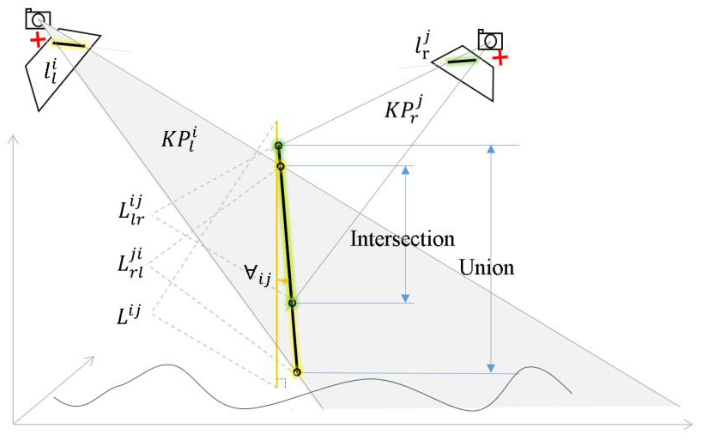
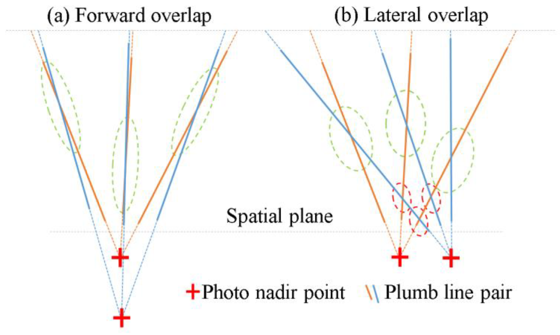
2.2. Spatial Constraint

Photos with position and pose can be mapped to any spatial plane by constructing affine transformation parameters through the perspective camera model $C$. The pixel coordinates of the photo’s four corner points are set as $\left\{p^n\right\}$. Through $C$, the inverse calculation is conducted to obtain four spatial lines $\left\{L^n\right\}$, which intersect with the spatial plane of elevation $\mathrm{Z}$ to obtain four points $\left\{P^n\right\}$. The correspondence between $\left\{p^n\right\}$ and $\left\{P^n\right\}$ could calculate the affine transformation matrix $\mathrm{H}=\left[\left[a_{11} a_{12} b_1\right]\left[a_{21} a_{22} b_2\right]\left[0 0 1\right]\right]$. Any point $p^k={\left[x^k,y^k\right]}^T$ in the photo can be mapped to the elevation $Z^k$ spatial plane $S{P}^k$ via Equation (3), and then, the corresponding point $P^k={\left[X^k,Y^k,Z^k\right]}^T$ can be obtained.

$$\left[\begin{array}{c}{X}^k\\ Y^k\\ Z^k\end{array}\right]=\left[\begin{array}{ccc}{a}_{11}& a_{12}& b_1\\ a_{21}& a_{22}& b_2\\ 0& 0& Z^k\end{array}\right]\left[\begin{array}{c}{x}^k\\ y^k\\ 1\end{array}\right]$$

(3)

The closer the $Z^k$ is to the $p^k$ corresponding object point elevation, the closer $P^k$ is to the corresponding object point. The positions of the homologous points overlap after being projected onto the space plane where the corresponding object is located.

As for the line segments, as shown in Figure 6, photo line segments $l_l^i$ and $l_r^j$ are taken as a set of homonymous lines of spatial line segment $L_g$, and $L_l^{hi}$ and $L_r^{hj}$ as their projected line segments in the spatial plane $S{P}_h$ with elevation $h$. If $h$ is within the elevation range of $L_g$, $L_l^{hi}$ and $L_r^{hj}$ exist at least at one point. $SP{P}_l^{hi}$ and $SP{P}_r^{hj}$ can be restored to the real position respectively, which represents the same object and overlaps with each other. $SP{P}_l^{hi}$ and $SP{P}_r^{hj}$ are homonymous points constrained by the same position and, accordingly, are named SPPs (Same Position Homonymous Points).

The probability of obtaining SPPs after homonymous line projection is proportional to the elevation range of its corresponding spatial line segment under uniform spatial stratification. Plumb lines possess a more extensive elevation range than others. Thanks to this property, the projection of their homonymous lines can ensure the existence of true SPPs in a certain density of stratified spatial planes.

Ground elevation range was obtained from the connection points previously to construct the spatial plane set $\left\{S{P}_h\right\}$ with equal elevation difference (0.1 m in this paper). Then, the set of plumb lines $\left\{l_l^i\right\}$ and $\left\{l_r^j\right\}$ was projected to $\left\{S{P}_h\right\}$ via Equation (3) to obtain the set of spatial line segments $\left\{L_l^{hi}\right\}$ and $\left\{L_r^{hj}\right\}$. Finally, the SPPs set $\left\{SP{P}^{hij}\right\}$ could be obtained by calculating their intersections. Figure 7 shows an instance of the SPPs calculation process.

SPPs compress the search domain of homonymous plumb lines as the spatial constraint. However, it is merely a necessary and insufficient condition for homonymous plumb-line determination. As shown in Figure 6 and Figure 7d, the false SPPs are generated between the adjacent plumb lines. Therefore, neighborhood color is selected as the feature descriptor to determine further whether plumb lines are homonymous.

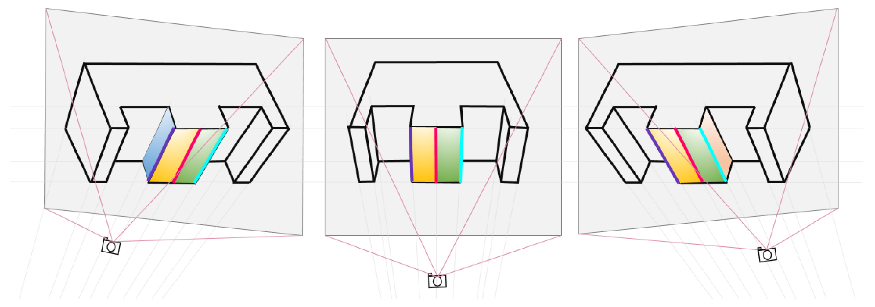
2.3. Feature Description

MSLD and LBD are classic line segment descriptors. MSLD counts the gradient vectors in 4 directions in each sub-region of the pixel support region to construct the descriptor matrix, while LBD divides the support domain of the line segments into multiple strips, counts the pixel gradient, and calculates the mean vector and standard deviation of the statistics as the descriptor matrix. They construct the support domain based on pixels and count multiple features with higher dimensionality and more uniqueness, but they are more sensitive to consistency and compression distortion on homonymous lines.

In comparison, color is more resistant to inconsistency, shape and scale change, etc., than higher dimensional descriptors, e.g., MSLD and LBD. As shown in Figure 2 and Figure 8, color can encompass all features in the plumb line’s neighborhood. Thus, the both-side neighborhood primary colors of the plumb line were extracted as descriptors for the homonymy determination.

As shown in Figure 8, two problems arise in the process of comparing the homonymous plumb-line neighborhood colors: the variability of brightness caused by the capture angle and illumination direction; and the instability of mixed colors caused by the change in pixel-corresponding spatial domain.

To reduce the impact of color variation on consistent determination, the colorimetry method was adopted to calculate values of the chromatic aberration instead of the Euclidean distance of RGB. Furthermore, the whole one-side neighborhood is regarded as a basic unit, thus expanding the spatial domain and weakening the mixed color instability problem.

2.3.1. Calculation of Chromatic Aberration

Colorimetry relates human subjective color perception to objective physical measurements, which uses the Lab (luminance, red/green difference, yellow/blue difference) color space. The CIEDE2000 is regarded as the best mutual matching chromatic aberration formula with human vision in theory currently [46,47,48,49]. Lab and CIEDE2000 are employed in this paper to extract and compare the plumb-line neighborhood primary colors.

2.3.2. Partitioning and Extraction of Neighborhood Pixels

Polar coordinate systems centered on each photo nadir point were constructed to partition and extract the plumb-line neighborhood pixels, as shown in Figure 9.

The neighborhoods of the homonymous plumb lines correspond one-to-one in the clockwise and anti-clockwise regions divided by the observation vector. The image of $phot{o}_l$ can be taken as an example. As shown in Figure 9, $R_l^i$, which is the vector from photo nadir points $p_l^{pnp}$ to the 2D plumb lines $l_l^i$, is the mapping of the observation vector from the photography center to the 3D plumb line $L^{ij}$ in the photos. When $L^{ij}$ is observed in both $phot{o}_l$ and $phot{o}_r$, their same-side neighborhoods are on the same side of the observation vector $R_l^i$ and $R_r^j$. Therefore, polar coordinates were established, and the neighbors of the plumb line were partitioned according to the clockwise and anti-clockwise regions in polar coordinates to achieve the correspondence of the homonymous plumb line’s same-side neighborhoods.

The distortion of the plumb-line neighborhoods varies among different photos. Thus, pixels cannot be acquired accurately by panning plumb lines. The plumb-line clockwise and anti-clockwise neighboring pixel sets $\left\{Pi{x}_l^i\right\}$ were extracted, respectively, based on the polar coordinate system of each image, as shown in Figure 9, using Equation (4).

$$\left\{Pi{x}_l^i\right\}=\{\begin{array}{c}{\displaystyle \sum }_{d=1}^2{\rm T}\left(Rotate\left(l_l^i,\exists \times \frac{\left(d+\tau \right)}{r}\right)\right) \\ {\rm T}\left(Rotate\left(l_l^i,\exists \times \frac{\Delta \theta }{2}\right) \right) if epl\end{array}$$

(4)

where the ${\rm T}\left(l\right)$ function extracts the pixels which through the line segment $l$, $Rotate\left(l_l^i,\theta \right)$ rotates the plumb line $l_l^i$ by arcdegree $\theta$ around the photo nadir point $p_l^{pnp}$; $\exists$ denotes the rotation direction parameter (−1 for clockwise; 1 for anti-clockwise); $d$ is the pixel distance of $l_l^i$ rotation (1 and 2 are chosen in this paper); $\tau$ represents the distance increment to avoid the mixed pixels generated by the drastic color change near the plumb line (0.5 is chosen in this paper); $r=Max\left(Distance\left(p_l^{pnp},l_l^i\right)\right)$ calculates the greater of the distances from the two endpoints of $l_l^i$ to $p_l^{pnp}$; $if epl$ represents the situation that another plumb line $l_l^{i2}$ exists in the neighborhood region formed by $l_l^i$ rotated by 3 pixels, and $\Delta \theta$ is the absolute value of the azimuthal difference between $l_l^i$ and $l_l^{i2}$.

After extracting the plumb line, the set of pixels in each line’s clockwise and anti-clockwise neighborhoods was recorded separately. The pixels were converted from RGB to Lab color space before proceeding to the next step of color feature description.

2.3.3. Description of Pixel Color Feature

The primary color was extracted as the descriptor of the neighborhood color. After extracting the plumb line $l_l^i$ clockwise or anti-clockwise neighborhood pixel set $\left\{Pi{x}_l^i\right\}$ via Equation (4), the pixels with the largest chromatic aberration from the average value were eliminated until the chromatic aberration of each pixel was within 6.0 from the average value or the number of remaining pixels was less than 70%. Lab mean values of the remaining pixels in $\left\{Pi{x}_l^i\right\}$ were employed as the primary color. Finally, the plumb line neighborhood clockwise and anti-clockwise primary colors $\left\{l_l^i.{\overline{lab}}_c\right\}$ and $\left\{l_l^i.{\overline{lab}}_{ac}\right\}$ were collected.

2.3.4. Consistent Determination of the Primary Color

Plumb lines are mainly located on the structure’s facade, and their visible angles are distributed within the facade orientation. As shown in Figure 10, with the gradual change in the observation view, the plumb-line neighborhood observations keep the single-side consistency in the edge structure plumb line (blue and cyan) and the both-side consistency in the middle structure plumb line (red).

As shown in Figure 11, neighborhood inconsistency on both sides appears when the observation vectors are located in the second and fourth quadrants (Q2 and Q4), respectively, where they form a pair of views (red observation vectors).

However, the observations of plumb-line both-side neighborhoods are rarely inconsistent, especially in the photos obtained from oblique photogrammetry tasks. In terms of the observation angle, the photography center is far higher than the captured building. Regarding realistic scenes, building structures almost always have right or obtuse angles.

Hence, the consistency of at least a single neighborhood observation could be an important basis for the match. SPCC (Single-Side Primary Color Consistency) was regarded as the basic requirement for determining the plumb-line homonyms and was calculated via Equation (5).

$$\mathrm{SPCC}=ToF\left[\Delta E_{00}\left(l_l^i.{\overline{lab}}_c,l_r^j.{\overline{lab}}_c\right) \left|\right| \Delta E_{00}\left(l_l^i.{\overline{lab}}_{ac}-l_r^j.{\overline{lab}}_{ac}\right)<6.0\right]$$

(5)

where $ToF$ denotes the True or False determination function; $\Delta E_{00}$ is the CIEDE2000 color aberration calculation formula; $l_r^j.{\overline{lab}}_c$ and $l_r^j.{\overline{lab}}_{ac}$ represent the clockwise and anti-clockwise neighborhood primary colors of plumb line $l_r^j$ of another image $phot{o}_r$, respectively.

2.4. Initial Matching

The initial matching of plumb lines was implemented based on the SPPs and primary color descriptors extracted in the previous sections.

The number of SPPs positively correlates with the probability of a plumb-line pair correct match. Accordingly, the greedy strategy was adopted regarding the plumb-line pair with the largest SPP number and the SPCC as the local optimal solution. The plumb-line pair $l_l^i$ and $l_r^j$ was traversed and recorded in $\left\{SP{P}^{hij}\right\}$ from the highest to the lowest according to the count of SPPs. If neither was recorded and SPCC was equal to true, then it should have been recorded to the initial set of matching results ${\left\{\langle l_l^i,l_r^j\rangle \right\}}^1$. The greedy strategy significantly reduced the computation and completed the initial matching with only once $\left\{SP{P}^{hij}\right\}$ traversal.

2.5. Error Rejection

The motion vector field of the initial matching results is too smooth to be purified by classical algorithms such as RANSAC [50] and VFC [51]. The trifocal tensor constraint is a commonly validated method in the line-matching algorithm under the positional constraint. However, this paper still expects to exploit the potential of line matching under two photos to reduce the computational complexity and improve the generalization.

The credibility of the matching results was gauged by the IoU (Intersection over Union) and verticalness of $L_{lr}^{ij}$. As shown in Figure 12, it was calculated by plumb-line spatial solution triangle intersection.

2.5.1. IoU Filtering

The IoU represents the inconsistency of the plumb-line pair, which is positively related to the correctness of the matching result, calculated via Equation (6).

$$Io{U}_{ij=}Min\left(\begin{array}{c}Abs\left(\frac{L_{lr}^{ij}.Zmin-L_{rl}^{ji}.Zmax}{L_{lr}^{ij}.Zmax-L_{rl}^{ji}.Zmin}\right)\end{array},Min\left(\frac{len\left(L_{lr}^{ij}\right)}{len\left(L_{rl}^{ji}\right)},\frac{len\left(L_{rl}^{ji}\right)}{len\left(L_{lr}^{ij}\right)}\right)\right)$$

(6)

As shown in Figure 12, $L_{lr}^{ij}$ and $L_{rl}^{ji}$ are the spatial plumb lines corresponding to the plumb lines $l_l^i$ and $l_r^j$, which are derived from the intersection of the spatially solved triangles $K{P}_l^i$ and $K{P}_r^j$ obtained by the inverse-perspective functions $C_l^{-1}$ and $C_r^{-1}$. They can be calculated via Equation (7).

$$\{\begin{array}{c}K{P}_l^i=C_l^{-1}\left(l_l^i\right) \\ K{P}_r^j=C_r^{-1}\left(l_r^j\right) \\ L_{lr}^{ij}=Intersect\left(K{P}_l^i,Panel(K{P}_r^j)\right)\\ L_{rl}^{ji}=Intersect\left(Panel\left(K{P}_l^i\right),K{P}_r^j\right)\end{array}$$

(7)

The function $Panel()$ solves for the plane where the spatial triangle is located, and the function $Intersect()$ solves for the intersection line of two spatial planes. The solution with IoU less than 0.3 was regarded as poor confidence and then eliminated from the initial matching ${\left\{\langle l_l^i,l_r^j\rangle \right\}}^1$, and the IoU filtering result ${\left\{\langle l_l^i,l_r^j\rangle \right\}}^2$ was obtained subsequently.

2.5.2. Verticalness Filtering

The angular deviation ${\forall }_{ij}$ of the spatial plumb line $L_{lr}^{ij}$ from the ideal spatial plumb line $L^{ij}$ (as shown in Figure 12) was calculated as an evaluation indicator of verticalness via Equation (8).

$${\forall }_{ij}={\forall }_{ji}=acos\left(\left(L_{lr}^{ij}.Zmax-L_{lr}^{ij}.Zmin\right)/\left(len\left(L_{lr}^{ij}\right)\right)\right)$$

(8)

The matching results of the incorrectly homonymous plumb lines are always featured with larger ${\forall }_{ij}$. However, the verticalness of spatial lines cannot be determined by fixed thresholds. Firstly, the plumb structural feature lines are not exactly parallel to the plumb lines; secondly, deviations exist between the matched and original spatial line due to the influence of positional accuracy, photographic baseline, camera distortion, etc. This results in different photo combinations corresponding to different verticalness thresholds.

However, after eliminating the gross errors, the overall deviations should satisfy the normal distribution. The angular deviation set $\left\{{\forall }_{ij}\right\}$ was obtained after iterating through ${\left\{\langle l_l^i,l_r^j\rangle \right\}}^2$, and the errors were finally eliminated via Equation (9).

$$\{\begin{array}{c}\left\{{\forall }_{ij}^o\right\}=\{\begin{array}{c}OTSU\left(\left\{{\forall }_{ij}\right\}\right) if gross errors exist\\ \left\{{\forall }_{ij}\right\} else \end{array} \\ \left\{{\forall }_{ij}^s\right\}=\left\{{\forall }_{ij}^o\right\}<\left(\mu \left(\left\{{\forall }_{ij}^o\right\}\right)+2\sigma \left(\left\{{\forall }_{ij}^o\right\}\right)\right) \end{array}$$

(9)

where $\left\{{\forall }_{ij}^o\right\}$ denotes the set after the gross errors being removed from $\left\{{\forall }_{ij}\right\}$. The number is counted from $\left\{{\forall }_{ij}\right\}$ which is over 30°; If it is more than 5%, then gross errors are conjectured to exist. In this case, OTSU is firstly applied to obtain $\left\{{\forall }_{ij}^o\right\}$ (select the smaller of the two sets). Otherwise, $\left\{{\forall }_{ij}^o\right\}$ can be directly set equal to $\left\{{\forall }_{ij}\right\}$. $\left\{{\forall }_{ij}^s\right\}$ is the fraction of $\left\{{\forall }_{ij}^o\right\}$ that is less than the mean ($\mu$) plus the twice standard deviation ($2\sigma$), and its corresponding plumb-line pairs are identified as the final matching result ${\left\{\langle l_l^i,l_r^j\rangle \right\}}^3$.

3. Experiment and Discussion

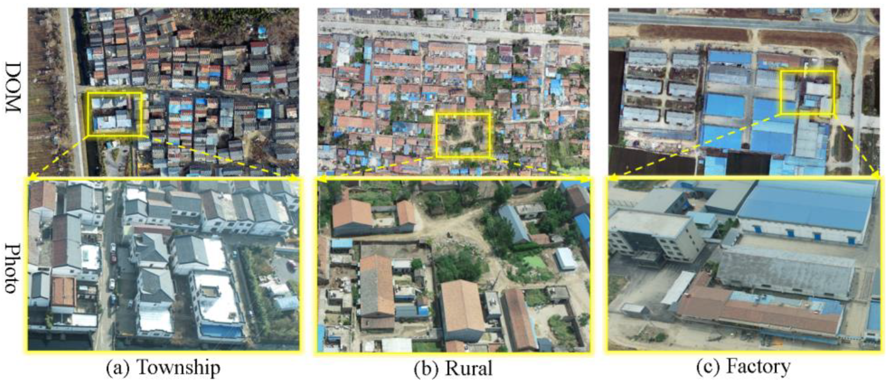
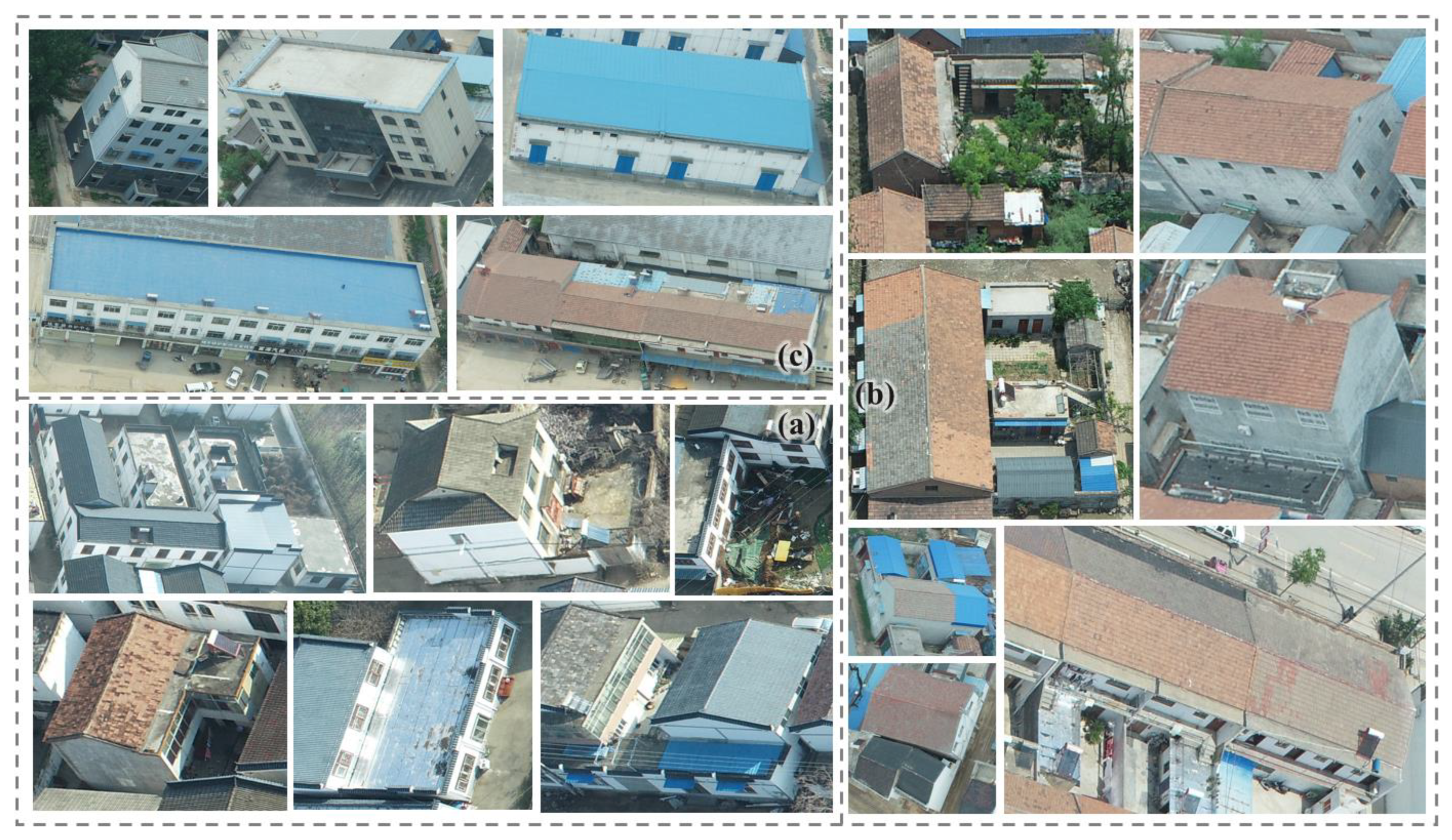
3.1. Data

The initial motivation was to extract and match plumb lines to optimize the process and products of UAV oblique photogrammetry, especially for the surface mesh’s optimization of 3D real-scene models of buildings. Hence, the UAV oblique photos and aero triangulation results from different production tasks (as shown in Figure 13) are selected as experimental data. As shown in the building examples in Figure 13 and Figure 14, there is a wide variety of buildings in the experimental area, and each building has a significantly different architectural style.

The photo acquisition device was DJI PHANTOM 4 RTK (DJI, Shenzhen, China) with a resolution of $5472\times 3648$ pixels (the main parameters of the aircraft and camera are shown in

Table 1. Main parameter table of DJI PHANTOM 4 RTK.

Aircraft		Camera		Platform
Type	Four-axis aircraft	Image sensor	1-inch CMOS; 20 million effective pixels	Controlled rotation range	Pitch: −90° to +30°
Hovering accuracy	±0.1 m	Camera Lens	FOV 84°; 8.8 mm/24 mm; Aperture f/2.8–f/11	Stabilization system	Three-axis (pitch, roll, yaw)
Horizontal flight speed	$\le 50 \mathrm{km}/\mathrm{h}$	Photo resolution	5472 × 3648 (3:2)	Maximum control speed	Pitch: 90°/s
Single flight time	Approx. 30 min	Photo format	JPEG	Angular jitter	±0.02°

, and the flight task parameters for data collection are shown in

Table 2. UAV Flight task parameters for data collection.

Parameter	Region a	Region b	Region c
Flight height	120 m	100 m	110 m
Photography angle	−45 degrees	−45 degrees	−50 degrees
Lateral overlap rate	70%	70%	70%
Forward overlap rate	80%	80%	80%

). The GET3D Cluster 5.0 was used to perform aerial triangulation of the UAV image set and obtain the position and posture information and connection points of the images.

3.2. Matching Photo Pair Selection

UAV oblique aerial photogrammetry requires a well-designed flight path that allows the camera to cover the target region and obtain photos that satisfy the requirements for the 3D reconstruction. In wide-scale oblique aerial photography missions, multi-oriented flying is one of the most common methods. As shown in Figure 15, UAVs normally fly along parallel flight strips at a fixed height and speed.

The overlap of consecutive photos within the same flight strip, known as forward overlap, satisfies the requirement of stereoscopic vision and requires a high degree of overlap; the overlap of photos between two adjacent flight strips, known as lateral overlap, satisfies the requirement of connecting adjacent flight strips and requires a low degree of overlap. The degree of photo overlap is a basic flight parameter, where the degree of forward overlap determines the interval for taking photos, while the degree of lateral overlap determines the spacing of the adjacent flight strips. In the experiment, the forward and lateral overlap of the photographic missions are set to 80% and 70%, respectively, which are commonly used empirical settings for UAV oblique photography used for 3D real-scene models of buildings.

Forward and lateral overlap are the two basic types of overlap of photo pairs in UAV oblique photogrammetry. Since the target area is not necessarily regular, the UAV takes photographs at fixed intervals along the flight strip during the mission. As a result, adjacent photos in one flight strip (forward overlap) basically move only forward–backward, and adjacent photos in neighboring flight strips (lateral overlap) move both left–right and forward–backward.

For the purpose of extracting and matching plumb lines, photos with forward overlapping are sufficient. However, to verify the performance and generalization of the algorithm, we simultaneously selected photos with forward and lateral overlapping in three representative scenes: township; rural; and factory.

3.3. Result

Similar oblique image line-matching algorithms that are also oriented toward the plumb line have not yet been found, so the performance of the algorithm could not be verified in the form of directly comparing the experimental results. Therefore, this paper firstly realizes all line matching by two types of matching algorithms based on BinaryDescriptor (traditional method based on line descriptor, encapsulated in OpenCV, hereinafter referred to as “BD”) and line transformers (deep learning method, hereinafter referred to as “LT”), and then extracts the correctly matched plumb-line pairs and displays the detailed images of the same region and statistically counts the correctly detected plumb lines to indirectly demonstrate the advantages of the proposed algorithm (hereinafter referred to as “Our”) in plumb-line matching.

Figure 16, Figure 17 and Figure 18 show the matching results. The experimental result graph is divided into three regions: the top is the experimental result of Our; the bottom left is the experimental result of BD; and the bottom right is the experimental result of LT. In the experimental results graph of Our, the upper half of “DOM Vision” and “Photo Vision” matching results correspond to the SPPs in DOM and the homonymous plumb lines in photos, respectively, where greens are the correct and reds are the wrong matching results; the bottom half “Detail” is the screenshot of matching details with the same scale; the homonymous plumb lines are marked with the same color. In the experimental result graphs of BD and LT, correctly matched plumb lines are connected with green connecting lines.

Most walls in the township scene a (Figure 16) are white, with gray edges. The advantage of the primary color of the line neighborhood as a descriptor is demonstrated, and the poor texture turns into a strong descriptor. The proposed algorithm accurately confronts the combined distortion of plumb-line rotation and compression. In addition, a1 shows a good detection rate of the plumb lines on the building facade, where extremely tight plumb lines are also correctly matched. Most of the line segments matched by BD and LT were parallel to the ground, and very few plumb lines perpendicular to the ground were successfully matched (as shown in

Table 3. Statistical table of the quantity of correctly matched plumb lines of different algorithms.

Forward Overlap				Lateral Overlap
Scene	Our	BD	LT	Scene	Our	BD	LT
a1	884 (913)	83 (1908)	0 (345)	a2	374 (470)	1 (4437)	0 (191)
b1	309 (316)	25 (1380)	0 (133)	b2	131 (168)	0 (1039)	0 (75)
c1	530 (542)	91 (1268)	7 (168)	c2	203 (265)	2 (1087)	0 (59)
Total	1723 (1771)	198 (4556)	7 (646)	Total	708 (903)	3 (6563)	0 (325)

).

The proposed algorithm is well-adapted to the rural scene b (Figure 17) in which the plumb-line neighborhood has complex and variable colors and serious endpoint inconsistencies. Some of the plumb lines in the BD algorithm are involved in matching, but a large number of mismatches are generated because of the similarity of building structures and textures. In the LT algorithm, almost no plumb lines are involved in the match and are successfully matched.

Factory scene c (Figure 18) includes various buildings, e.g., office buildings, factories, dormitories, etc. In c1, the correct matching of lines with similar geometry and texture on the left side verifies the strength of the SPPs’ spatial constraints; the accurate matching of the edge plumb lines existing in house corners and utility pole edges on the right side illustrates the applicability of the SPCC determination criterion in the case of complex changes in the background.

The statistics of the number of plumb lines correctly matched by the three algorithms are shown in Table 3, with the total number of matched line segments in parentheses.

Algorithms BD and LT show poor performance in plumb-line matching. The similar architectural structure of the building facades caused a large number of false matches for the BD algorithm, and only some plumb lines were successfully matched in the forward overlap experiments. The LT algorithm shows a poor adaptation to the experimental data, with a low number of detections in which essentially no plumb lines were successfully matched. The two line matching algorithms, BD and LT, were unable to extract high-quality homonymous plumb-line pairs. In comparison, the proposed algorithm shows a high level in both quantity and correct rate in plumb-line matching. Our plumb-line matching algorithm can be applied as a complement to other all-line matching algorithms.

Table 4. Statistical table of the quantity and accuracy of the proposed algorithm.

Forward Overlap				Lateral Overlap
Scene	Correct	Sum	Accuracy	Scene	Correct	Sum	Accuracy
a1	884	913	96.82%	a2	374	470	79.57%
b1	309	316	97.78%	b2	131	168	77.98%
c1	530	542	97.79%	c2	203	265	76.60%
Total	1723	1771	97.29%	Total	708	903	78.41%

shows the detailed statistics of the quantity and correct rate of the proposed algorithm in plumb-line matches.

From the point of view of accuracy, the average values in the forward and lateral overlap photos reach 97.29% and 78.41%, respectively. The former is higher than the latter, and both keep stability. From the view of quantity, the total numbers in the forward and lateral overlap photos are 1723 and 708, respectively. The former is higher than the latter, varying significantly between different scenes.

Overall, the proposed algorithm still performs well under the two broad criteria of 30% IoU threshold and SPCC, especially in heading overlap, which is trustworthy.

Matching results with high IoU or BPCC (both-side primary color consistency) possess higher accuracy, especially for lateral overlap experiments.

Table 5. Statistical table of quantity and accuracy changes in the proposed algorithm.

IoU	Forward Overlap						Lateral Overlap
	SPCC			BPCC			SPCC			BPCC
	Correct Sum Accuracy			Correct Sum Accuracy			Correct Sum Accuracy			Correct Sum Accuracy
0.3	1723	1771	97.29%	1435	1441	99.58%	708	903	78.41%	305	326	93.56%
0.4	1688	1728	97.69%	1414	1419	99.65%	672	829	81.06%	293	311	94.21%
0.5	1600	1633	97.98%	1347	1351	99.70%	614	734	83.65%	274	288	95.14%
0.6	1473	1495	98.53%	1256	1259	99.76%	543	620	87.58%	237	248	95.56%
0.7	1289	1305	98.77%	1103	1105	99.82%	450	493	91.28%	193	201	96.02%
0.8	983	996	98.69%	843	844	99.88%	332	358	92.74%	150	155	96.77%
0.9	506	513	98.64%	437	437	100.00%	175	178	98.31%	81	81	100.00%

and Figure 19 show the accuracy and quantity variation statistics of filtered experimental results under different IoU and primary color consistency determination criteria.

As the IoU rises, the accuracy displays an upward trend. As shown in Figure 19a, the forward overlap photo accuracy is consistently high, with the SPCC results ranging from 97% to 99%, BPCC results above 99.5%, and BPCC results reaching 100% at the IoU of 0.9. The lateral overlap photo accuracy improves significantly with the rise in IoU, showing a linear increase with a high speed, with the SPCC results rising from 78.41% to 98.31% and BPCC results from 93.56% to 100%. With the IoU rising, the quantity decreases at different rates. As shown in Figure 19b, the forward overlap photo correct matching quantity displays an exponential decreasing trend, and the final reduction quantity declines to 70.6% (SPCC) and 69.5% (BPCC). While lateral overlap photo correct matching quantity shows a smooth decreasing trend, the final reduction quantity reaches 75.3% (SPCC) and 73.4%(BPCC), respectively.

The BPCC results are included in the SPCC. The accuracy of BPCC results is significantly higher than that of SPCC, especially for lateral overlap photos. In forward overlap photos, BPCC result accuracy increases by 2.36–1.38%, compared with that of SPCC. In lateral overlap photos, the BPCC result accuracy increases by about 10%; especially at the start IoU of 0.3, it rises from 78.41% to 93.56% (an increase of 15.15%). The growth rate decreases gradually with the rise in IoU. The quantity of BPCC results accounts for about 85% (forward overlap) and 45% (lateral overlap), respectively.

The BPCC reduces the quantity but improves the accuracy significantly, especially for the lateral overlap photos. The proposed algorithm exhibits advanced performance in forward overlap photo matching experiments. As for the lateral overlap photos, the accuracy could be improved by screening high IoU (around 0.5) or BPCC results.

Overall, the proposed plumb-line matching algorithm performed well in different experimental scenes and could produce trustworthy building 3D plumb lines. An average accuracy of over 97% was achieved in the forward overlap photo experiments, and the BPCC results in the lateral overlap photo experiments reached an accuracy of over 93%. Moreover, the algorithm performed stable and high accuracy on the building facade despite the occlusion, structural distortion, and simple appearance, showing strong adaptability to inconsistency, rotation, scale, and poor texture.

3.4. Discussion

Verticality is the most important characteristic of a building and is the basis for ensuring its stability and safety. Therefore, even how irregular the shape of a building is, the plumb line in it is necessarily very regular. As a result, the proposed algorithm shows high accuracy stability in different matching scenes. The unique status of plumb lines in buildings ensures the algorithm’s generalization even in terms of complex building scenarios that are regular in height or shape. The experimental results demonstrate that SPPs and SPCC are reliable techniques for homonymous plumb-line determination. The proposed algorithm could solve the matching problem of building facades with high distortion and poor texture in oblique aerial photography.

When identifying plumb lines, it should be noted that the plumb lines calculated via Equation (2) are not always correct, as shown in Figure 5b. Generally, the longer the line segment and the smaller the deviation angle $\Delta \theta$, the higher the probability of obtaining the correct result. However, line segments of all lengths were still chosen, and a higher tolerance was adopted on the determination threshold of $\Delta \theta$, because the correspondence of the homologous plumb lines possesses the highest priority among the factors affecting the matching accuracy. To be specific, more lines were allowed to be involved in the matching at the beginning to ensure good correspondence of the homologous lines. But at the same time, the strict screening was executed at the end to improve the normality of the matching results. This improved the matching accuracy and ensured the geometric properties of matching results, positively affecting the subsequent applications.

When calculating SPPs by spatial layered projection, we chose 0.1 m as the layer interval. This means that there will be the same position homonymous point when the building structure represented by the plumb-line pair is above 0.1 m. However, theoretically, the finer the spatial layering, the more accurate the judgment of the spatial constraint strength by the number of SPPs. But this also means higher computation. Balancing the density of layering, computation, and matching accuracy and studying other SPP calculation methods, such as partition projection and classification projection, are important future research directions.

When describing the features of the plumb lines, we use the primary color as the descriptor. The following strategy was adopted to make the color description more accurate. First, we rotate the plumb line around the photo nadir point to ensure the accuracy of extracted pixels. Second, we use 1.5 and 2.5 pixels as the rotation values to avoid the mixed pixels from the plumb line itself and adjacent structures and make the pixels from the same structure. Finally, we eliminate the noise through iteration and then extract the primary color. This ensures the consistency of the extraction objects and the generality of the extraction method.

Taking plumb lines as targets actually simplifies the line-matching problem. The complexity of the matching problem is transformed from $N_l\times N_r$ to $N_l\times r_l\times N_r\times r_r$ (where $N_l$ and $N_r$ are the number of line segments in the image pair, and $r_l$ and $r_r$ are the proportion of plumb lines in it). Definitely, $r_l$ and $r_r$ are both less than 1 (in the experimental data, the plumb-line ratio is generally less than 0.1). Therefore, the algorithm has inherent advantages in theory and complexity compared to the algorithm that matches all lines, which also makes the algorithm achieve high accuracy, especially in heading overlap matching.

However, the matching results in the forward overlap photos are significantly superior to those in the lateral overlap photos. Differences in spatial constraint ability and color consistency result in this outcome. The plumb line behaves as a line segment pointing to the photo nadir point. In terms of the spatial constraints of SPPs, the deformation of the homonymous plumb line in the forward overlap photos is mainly vertical compression (as shown in Figure 2b,d), and the homonymous plumb line intersects in the spatial plane of the SPPs with a small-angle “X” shape (as shown in Figure 20a), the probability of intersecting with neighboring plumb lines to produce erroneous SPPs is low. Whereas the deformation of the plumb lines in the lateral overlap photos contains both vertical compression and left-right distortion (as shown in Figure 2a,c), and the homonymous plumb lines are intersected in the spatial plane of the SPPs with a large-angle “X” shape (as shown in Figure 20b), and neighboring plumb lines are more likely to produce erroneous SPPs. In terms of the degree of color consistency, the observation angle of the neighbors of the homonymous plumb line in the forward overlap image is less variable, and the color consistency is higher (as shown in Figure 2b,d). While the observation angle of the neighbors of the homonymous plumb line in the lateral overlap photo is more variable, the color is prone to lightness-dominated color changes, and the consistency is relatively lower (as shown in Figure 2a,c). Those lead to the resulting forward overlap experiments possessing a fairly high accuracy, while the lateral overlap performance is mediocre. Future research needs to focus on optimizing the SPPs constraint and SPCC calculation method, which can be applied to the lateral overlap photos to improve the matching quantity and accuracy.

Finally, the current version of the algorithm extracts and matches homonymous plumb lines from combinations of the same shoot direction photos taken during UAV mapping production missions. The future research direction is to improve and enhance the performance of the plumb-line matching algorithm in a wider range of application scenarios. Designing more reasonable and diversified combinations of images and optimizing the matching process by considering the geometric distribution and matching cost between plumb-line pairs are the next research contents.

4. Summary

Building facade is always a weak region for traditional matching methods in oblique photogrammetry. The plumb line and the weak texture, non-Lambertian objects, deformation, and occlusion regions in the building facade have a strong spatial correlation. Extracting and matching plumb lines can provide suggestions for selecting key points used for aerial triangulation and dense matching, thereby optimizing the process and products of oblique photogrammetry. Thus, we proposed a novel matching algorithm oriented to plumb lines based on the hybrid constraints of spatial and color elements. The main contributions of this study are summarized below.

First, we proposed the spatial constraints unique to plumb lines—SPPs (Same Position Homonymous Points). Exploited the property of the high elevation range of plumb lines, calculated the SPPs between plumb-line pairs by their intersections in the projection plane, and quantitatively described their spatial constraints by the number of SPPs.

Second, we designed the criterion for plumb-line feature similarity judgment—SPCC (Single-side Primary Color Consistency). Designed a polar coordinate system with the photo nadir point as center, endowed plumb line’s both neighborhoods with direction parameter, extracted and compared the primary color of the neighbors on both sides by the colorimetric method, and relied on the property with at least a single side of the plumb-line neighbors from the aerial perspective visible at the same time to realize the similarity determination of plumb line’s features.

Third, we eliminated the matching errors based on IoU and verticalness filtering. To address the problem that the plumb line’s matching vector field is excessively smooth and the classical purification algorithm cannot be applied, rejected errors by the overall analysis of IoU and verticalness of matching results.

The proposed algorithm performed robustly in the different scene and view combinations, demonstrating advanced accuracy, especially in the forward overlap photos. Benefiting from the strategy of plumb-line oriented partial line matching, the proposed algorithm owns inherent advantages in theory and computational complexity, applicable to all building-oriented oblique photogrammetry tasks. It can solve the problems of the sparse and high-error traditional algorithms in matching building facades with occlusion, distortion, and poor texture in oblique photogrammetry tasks. The plumb lines convey explicit geometric information possessing high application value and potential. The algorithm boasts of great potential for further improvement. More efforts will be made to reduce the computational effort, improve the matching quantity and accuracy of the lateral overlap photos, and enhance the confidence evaluation method to explore broader application scenarios.

References

1. Nex, F.; Remondino, F. UAV for 3D mapping applications: A review. Appl. Geomat. 2014, 6, 1–15. [Google Scholar] [CrossRef]
2. Yang, B.; Ali, F.; Zhou, B.; Li, S.; Yu, Y.; Yang, T.; Liu, X.; Liang, Z.; Zhang, K. A novel approach of efficient 3D reconstruction for real scene using unmanned aerial vehicle oblique photogrammetry with five cameras. Comput. Electr. Eng. 2022, 99, 107804. [Google Scholar] [CrossRef]
3. Li, Q.; Huang, H.; Yu, W.; Jiang, S. Optimized views photogrammetry: Precision analysis and a large-scale case study in qingdao. IEEE J. Sel. Top. Appl. Earth Obs. Remote Sens. 2023, 16, 1144–1159. [Google Scholar] [CrossRef]
4. Jiang, S.; Jiang, C.; Jiang, W. Efficient structure from motion for large-scale UAV images: A review and a comparison of SfM tools. ISPRS J. Photogramm. Remote Sens. 2020, 167, 230–251. [Google Scholar] [CrossRef]
5. Che, D.; He, K.; Qiu, K.; Ma, B.; Liu, Q. Edge Restoration of a 3D Building Model Based on Oblique Photography. Appl. Sci. 2022, 12, 12911. [Google Scholar] [CrossRef]
6. Remondino, F.; Gerke, M. Oblique aerial imagery—A review. Photogramm. Week 2015, 15, 75–81. [Google Scholar]
7. Verykokou, S.; Ioannidis, C. Oblique aerial images: A review focusing on georeferencing procedures. Int. J. Remote Sens. 2018, 39, 3452–3496. [Google Scholar] [CrossRef]
8. Chen, L.; Rottensteiner, F.; Heipke, C. Feature detection and description for image matching: From hand-crafted design to deep learning. Geo-Spat. Inf. Sci. 2021, 24, 58–74. [Google Scholar] [CrossRef]
9. Wu, B.; Xie, L.; Hu, H.; Zhu, Q.; Yau, E. Integration of aerial oblique imagery and terrestrial imagery for optimized 3D modeling in urban areas. ISPRS J. Photogramm. Remote Sens. 2018, 139, 119–132. [Google Scholar] [CrossRef]
10. Wang, D.; Shu, H. Accuracy Analysis of Three-Dimensional Modeling of a Multi-Level UAV without Control Points. Buildings 2022, 12, 592. [Google Scholar] [CrossRef]
11. Wang, K.; Shi, T.; Liao, G.; Xia, Q. Image registration using a point-line duality based line matching method. J. Vis. Commun. Image Represent. 2013, 24, 615–626. [Google Scholar] [CrossRef]
12. Hofer, M.; Wendel, A.; Bischof, H. Line-based 3D reconstruction of wiry objects. In Proceedings of the 18th Computer Vision Winter Workshop, Hernstein, Austria, 4–6 February 2013; pp. 78–85. [Google Scholar]
13. Wei, D.; Zhang, Y.; Liu, X.; Li, C.; Li, Z. Robust line segment matching across views via ranking the line-point graph. ISPRS J. Photogramm. Remote Sens. 2021, 171, 49–62. [Google Scholar] [CrossRef]
14. Elqursh, A.; Elgammal, A. Line-based relative pose estimation. In Proceedings of the 2011 IEEE Conference on Computer Vision and Pattern Recognition, Colorado Springs, CO, USA, 20–25 June 2011; IEEE: New York, NY, USA, 2011; pp. 3049–3056. [Google Scholar]
15. Lee, J.H.; Zhang, G.; Lim, J.; Suh, I.H. Place recognition using straight lines for vision-based SLAM. In Proceedings of the 2013 IEEE International Conference on Robotics and Automation, Karlsruhe, Germany, 6–10 May 2013; IEEE: New York, NY, USA, 2013; pp. 3799–3806. [Google Scholar]
16. Shipitko, O.; Kibalov, V.; Abramov, M. Linear features observation model for autonomous vehicle localization. In Proceedings of the 2020 16th International Conference on Control, Automation, Robotics and Vision (ICARCV), Shenzhen, China, 13–15 December 2020; IEEE: New York, NY, USA, 2020; pp. 1360–1365. [Google Scholar]
17. Fan, B.; Wu, F.; Hu, Z. Line matching leveraged by point correspondences. In Proceedings of the 2010 IEEE Computer Society Conference on Computer Vision and Pattern Recognition, San Francisco, CA, USA, 13–18 June 2010; IEEE: New York, NY, USA, 2010; pp. 390–397. [Google Scholar]
18. Yoon, S.; Kim, A. Line as a Visual Sentence: Context-Aware Line Descriptor for Visual Localization. IEEE Robot. Autom. Lett. 2021, 6, 8726–8733. [Google Scholar] [CrossRef]
19. Ma, J.; Jiang, X.; Fan, A.; Jiang, J.; Yan, J. Image matching from handcrafted to deep features: A survey. Int. J. Comput. Vis. 2021, 129, 23–79. [Google Scholar] [CrossRef]
20. Forero, M.G.; Mambuscay, C.L.; Monroy, M.F.; Miranda, S.L.; Méndez, D.; Valencia, M.O.; Gomez Selvaraj, M. Comparative analysis of detectors and feature descriptors for multispectral image matching in rice crops. Plants 2021, 10, 1791. [Google Scholar] [CrossRef]
21. Sharma, S.K.; Jain, K.; Shukla, A.K. A Comparative Analysis of Feature Detectors and Descriptors for Image Stitching. Appl. Sci. 2023, 13, 6015. [Google Scholar] [CrossRef]
22. Schmid, C.; Zisserman, A. Automatic line matching across views. In Proceedings of the IEEE Computer Society Conference on Computer Vision and Pattern Recognition, San Juan, PR, USA, 17–19 June 1997; IEEE: New York, NY, USA, 1997; pp. 666–671. [Google Scholar]
23. Schmid, C.; Zisserman, A. The geometry and matching of lines and curves over multiple views. Int. J. Comput. Vis. 2000, 40, 199–233. [Google Scholar] [CrossRef]
24. Sun, Y.; Zhao, L.; Huang, S.; Yan, L. Line matching based on planar homography for stereo aerial images. ISPRS J. Photogramm. Remote Sens. 2015, 104, 1–17. [Google Scholar] [CrossRef]
25. Wei, D.; Zhang, Y.; Li, C. Robust line segment matching via reweighted random walks on the homography graph. Pattern Recognit. 2021, 111, 107693. [Google Scholar] [CrossRef]
26. Hofer, M.; Maurer, M.; Bischof, H. Efficient 3D scene abstraction using line segments. Comput. Vis. Image Underst. 2017, 157, 167–178. [Google Scholar] [CrossRef]
27. Zheng, X.; Yuan, Z.; Dong, Z.; Dong, M.; Gong, J.; Xiong, H. Smoothly varying projective transformation for line segment matching. ISPRS J. Photogramm. Remote Sens. 2022, 183, 129–146. [Google Scholar] [CrossRef]
28. Wang, Z.; Wu, F.; Hu, Z. MSLD: A robust descriptor for line matching. Pattern Recognit. 2009, 42, 941–953. [Google Scholar] [CrossRef]
29. Zhang, L.; Koch, R. An efficient and robust line segment matching approach based on LBD descriptor and pairwise geometric consistency. J. Vis. Commun. Image Represent. 2013, 24, 794–805. [Google Scholar] [CrossRef]
30. Vakhitov, A.; Lempitsky, V. Learnable line segment descriptor for visual slam. IEEE Access 2019, 7, 39923–39934. [Google Scholar] [CrossRef]
31. Lange, M.; Schweinfurth, F.; Schilling, A. Dld: A deep learning based line descriptor for line feature matching. In Proceedings of the 2019 IEEE/RSJ International Conference on Intelligent Robots and Systems (IROS), Macau, China, 3–8 November 2019; IEEE: New York, NY, USA, 2019; pp. 5910–5915. [Google Scholar]
32. Lange, M.; Raisch, C.; Schilling, A. Wld: A wavelet and learning based line descriptor for line feature matching. Proc. Intl. Symp. Vis. Mod. Vis. 2020, 39–46. [Google Scholar]
33. Ma, Q.; Jiang, G.; Lai, D. Robust Line Segments Matching via Graph Convolution Networks. arXiv 2020. [Google Scholar] [CrossRef]
34. Pautrat, R.; Lin, J.T.; Larsson, V.; Oswald, M.R.; Pollefeys, M. SOLD2: Self-supervised occlusion-aware line description and detection. In Proceedings of the IEEE/CVF Conference on Computer Vision and Pattern Recognition, Virtual, 19–25 June 2021; pp. 11368–11378. [Google Scholar]
35. Xiao, J. Automatic building outlining from multi-view oblique images. ISPRS Ann. Photogramm. Remote Sens. Spat. Inf. Sci. 2012, 1, 323–328. [Google Scholar] [CrossRef]
36. Gao, J.; Wu, J.; Zhao, X.; Xu, G. Integrating TPS, cylindrical projection, and plumb-line constraint for natural stitching of multiple images. Vis. Comput. 2023, 1–30. [Google Scholar] [CrossRef]
37. Wang, Z.; Li, X.; Zhang, X.; Bai, Y.; Zheng, C. An attitude estimation method based on monocular vision and inertial sensor fusion for indoor navigation. IEEE Sens. J. 2021, 21, 27051–27061. [Google Scholar] [CrossRef]
38. Tang, L.; Xie, W.; Hang, J. Automatic high-rise building extraction from aerial images. In Proceedings of the Fifth World Congress on Intelligent Control and Automation (IEEE Cat. No. 04EX788), Hangzhou, China, 15–19 June 2004; IEEE: New York, NY, USA, 2004; Volume 4, pp. 3109–3113. [Google Scholar]
39. Tardif, J.P. Non-iterative approach for fast and accurate vanishing point detection. In Proceedings of the 2009 IEEE 12th International Conference on Computer Vision, Kyoto, Japan, 29 September–2 October 2009; IEEE: New York, NY, USA, 2009; pp. 1250–1257. [Google Scholar]
40. Zhang, Y.; Dai, T.; Gao, S. Auto Extracting Vertical Lines from Aerial Imagery over Urban Areas. Geospat. Inf. 2009, 7, 4. [Google Scholar] [CrossRef]
41. Habbecke, M.; Kobbelt, L. Automatic registration of oblique aerial images with cadastral maps. In Trends and Topics in Computer Vision: ECCV 2010 Workshops, Heraklion, Crete, Greece, 10–11 September 2010, Revised Selected Papers, Part II 11; Springer: Berlin/Heidelberg, Germany, 2012; pp. 253–266. [Google Scholar]
42. Xiao, J.; Gerke, M.; Vosselman, G. Building extraction from oblique airborne imagery based on robust façade detection. ISPRS J. Photogramm. Remote Sens. 2012, 68, 56–68. [Google Scholar] [CrossRef]
43. Zhang, J.; Zhang, Y.; Fang, F. Absolute Orientation of Aerial Imagery over Urban Areas Combined with Vertical Lines. Geomat. Inf. Sci. Wuhan Univ. 2007, 32, 197–200. [Google Scholar]
44. Gioi, R.G.V.; Jakubowicz, J.; Morel, J.M.; Randall, G. LSD: A Fast Line Segment Detector with a False Detection Control. IEEE Trans. Pattern Anal. Mach. Intell. 2010, 32, 722–732. [Google Scholar] [CrossRef] [PubMed]
45. Tomasi, C.; Manduchi, R. Bilateral filtering for gray and color images. In Proceedings of the Sixth International Conference on Computer Vision, Bombay, India, 7 January 1998; IEEE: New York, NY, USA, 1998; pp. 839–846. [Google Scholar]
46. Pereira, A.; Carvalho, P.; Coelho, G.; Côrte-Real, L. Efficient ciede2000-based color similarity decision for computer vision. IEEE Trans. Circuits Syst. Video Technol. 2019, 30, 2141–2154. [Google Scholar] [CrossRef]
47. Kinoshita, Y.; Kiya, H. Hue-correction scheme considering CIEDE2000 for color-image enhancement including deep-learning-based algorithms. APSIPA Trans. Signal Inf. Process. 2020, 9, e19. [Google Scholar] [CrossRef]
48. Yang, Y.; Zou, T.; Huang, G.; Zhang, W. A high visual quality color image reversible data hiding scheme based on BRG embedding principle and CIEDE2000 assessment metric. IEEE Trans. Circuits Syst. Video Technol. 2021, 32, 1860–1874. [Google Scholar] [CrossRef]
49. Zheng, Y.; Xu, Y.; Qiu, S.; Li, W.; Zhong, G.; Chen, M.; Sarem, M. An improved NAMLab image segmentation algorithm based on the earth moving distance and the CIEDE2000 color difference formula. In Proceedings of the Intelligent Computing Theories and Application: 18th International Conference, ICIC 2022, Xi’an, China, 7–11 August 2022; Proceedings, Part I. Springer International Publishing: Cham, Germany, 2022; pp. 535–548. [Google Scholar]
50. Fischler, M.A.; Bolles, R.C. Random sample consensus: A paradigm for model fitting with applications to image analysis and automated cartography. Commun. ACM 1981, 24, 381–395. [Google Scholar] [CrossRef]
51. Ma, J.; Zhao, J.; Tian, J.; Yuille, A.L.; Tu, Z. Robust point matching via vector field consensus. IEEE Trans. Image Process. 2014, 23, 1706–1721. [Google Scholar] [CrossRef]
Figure 1. Examples of oblique photos and building 3D real-scene models. (a,b) show two examples with different styles of photographs and 3D real scene models, respectively. Building facade is always a weak region for traditional matching methods in oblique photogrammetry due to the many challenges, such as occlusion, deformation, weak texture, repetitive texture, and non-Lambertian objects. Therefore, the facade of the real 3D building model based on oblique photogrammetry generally has too many nodes and distorted structures. As can be seen, the plumb lines in the image generally appear in pairs, with their middle positions generally building structures such as exterior windows and terraces (where the glass is typically non-Lambertian object), and the rest of the neighborhood generally comprises walls (wall textures are mostly weak and repetitive). Therefore, the plumb lines have a close spatial relationship with these problem regions in both images and models.
Remotesensing 15 05290 g001
Figure 2. Examples of plumb lines in the photos from oblique photography tasks (screenshot at the same scale); (a,c) are from lateral overlap photo pair; (b,d) are from forward overlap photo pair. Plumb lines are particular line segments widely distributed in human activity scenes, especially on the facades of structures, e.g., building corners and door or window edges.
Remotesensing 15 05290 g002
Figure 3. Overall flowchart of the algorithm.
Remotesensing 15 05290 g003
Figure 4. Schematic of the vanishing points of parallel spatial lines in the photos. Extensions of parallel structural lines of the building intersect at the same vanishing point.
Remotesensing 15 05290 g004
Figure 5. Examples of plumb line back-calculation results in the photos. The red lines are the plumb line that back-calculates through the photo nadir point; (a,c) show two perfect back-calculation results where the plumb lines are extracted correctly. In comparison, some lines are incorrectly identified as plumb lines in (b), which are coincidentally oriented to the camera center.
Remotesensing 15 05290 g005
Figure 6. Schematic diagram of SPPs calculation. The yellow and green lines are the projections of the two photo line segments in different spatial planes using Equation (3); the “+” red circle represents the true SPPs, and the “x” red circle represents the false SPPs.
Remotesensing 15 05290 g006
Figure 7. Examples of the SPPs calculation process. The purple points are SPPs, and the spatial line segment elevation increases continuously from green to red. When the elevation of the spatial plane is within the elevation range of the plumb line, the homologous plumb lines will intersect, producing true SPPs. Therefore, SPPs can be used as positional constraints to determine the possible set of homologous plumb line pairs. But adjacent plumb lines may also intersect in the spatial plane, producing false SPPs.
Remotesensing 15 05290 g007
Figure 8. Examples of both-side neighborhood pixels of the plumb lines. Color is an essential feature of line-segment neighborhoods. Plumb lines mostly appear in the structural and color transition regions, with poor texture neighborhoods; (a,b) are from the forward and lateral overlap photos. Complex variations in the neighborhoods of the homonymous plumb lines lead to worse one-to-one correspondences between pixels. Thus, classical approaches, e.g., MSLD and LBD, are not applicable.
Remotesensing 15 05290 g008
Figure 9. Schematic diagram of plumb-line neighborhood pixels partitioning and extraction based on the photo polar coordinate system. The black line is the target plumb line, and the purple line is the other plumb line. The target is the plumb line l l i with yellow fluorescence, and R l i is the observation vector from the photo nadir point to the target. The l l i neighborhood pixels are partitioned by locating on the R l i clockwise or anti-clockwise region and are extracted by rotating l l i around p l p n p . The green and blue are the partitioning and extraction results of l l i clockwise and anti-clockwise neighborhood pixels, respectively.
Remotesensing 15 05290 g009
Figure 10. Schematic diagram of the consistency of the plumb-line neighborhoods under multi-view observation. When the observation view changes, the blue, red, and cyan plumb lines maintain at least single-side neighborhood consistency.
Remotesensing 15 05290 g010
Figure 11. Schematic diagram of the visible neighborhood of the plumb line under different observations. Colored arrows represent observation vectors. When the two observation vectors are located in the Q2 and Q4 quadrants (red arrows), respectively, the observations of the plumb-line neighborhood on both sides are inconsistent.
Remotesensing 15 05290 g011
Figure 12. Schematic diagram of plumb-line pairs forward intersection. K P l i and K P r j are the spatial solution triangles of plumb lines l l i and l r j , respectively.   L l r i j ,   L r l j i are their intersection lines with each other, which display certain overlapping and deviate from the standard spatial plumb line L i j with angular .
Remotesensing 15 05290 g012
Figure 13. Diagram of the experimental scenes. Photo (a) shows a township scene, in which the closely distributed buildings are of a single type, with an elevation range of 33.1–45.3 m; Photo (b) is a rural scene, in which the buildings are sparsely distributed and diverse in types, with an elevation range of 31.3–40.8 m; Photo (c) shows a factory scene, in which the buildings are distributed independently and are of complex types, with an elevation range of 30.6–51.5 m.
Remotesensing 15 05290 g013
Figure 14. Sample diagrams of buildings in different scenarios. The factory scene (c) contains taller factory dormitory buildings, medium-height office buildings, and lower factory buildings, all of which are distinctly different in terms of architectural appearance and building height; the township scene (a) and rural scene (b) do not vary much in height, but each has its own unique style in terms of building structure. Building facades in all scenes have weak textures, repeated textures, non-Lambertian objects (external windows), and occluded deformed regions.
Remotesensing 15 05290 g014
Figure 15. Schematic diagram of the UAV oblique-photography flight strips and the selection of experimental photo pairs. The green image pairs are forward-overlapping photo pairs (from the same flight strip, one in front and one behind), and the blue image pairs are lateral overlapping photo pairs (from neighboring flight strips, a combination of offsets perpendicular to and along the flight strip is generally present, but the former is generally much larger than the latter).
Remotesensing 15 05290 g015
Figure 16. Matching results of township scene a. In the DOM vision, the green circles and red crosses correspond to the SPPs (which are also the projection results of the spatial plumb lines generated by the forward intersection of the homologous plumb-line pairs) corresponding to the correct and erroneous plumb-line pair matching results, respectively. In the Photo and Detail visions, the homologous plumb-line pairs are shown in the same color. In the Photo vision, the green and red connecting lines correspond to the correct and erroneous matching results, respectively. Figure 17 and Figure 18 are similarly represented as such.
Remotesensing 15 05290 g016aRemotesensing 15 05290 g016b
Figure 17. Matching results of rural scene b.
Remotesensing 15 05290 g017aRemotesensing 15 05290 g017b
Figure 18. Matching results of factory scene c.
Remotesensing 15 05290 g018aRemotesensing 15 05290 g018b
Figure 19. Folding line graph of quantity and accuracy changes in the proposed algorithm.
Remotesensing 15 05290 g019
Figure 20. Schematic of the plumb-line projection in the space plane in the forward and lateral overlap experiments.
Remotesensing 15 05290 g020