Abstract
During gravity field modeling, the conventional acceleration approach rarely incorporates KBR inter-satellite range rate data from the GRACE mission. To propose an improved acceleration method, this study introduces initial orbital position and velocity vectors to be estimated along with a combination of Cowell, KSG, and Adams integrators. In addition to achieving a full-rank design matrix regarding orbit corrections when constructing observation equations, the proposed method is capable of utilizing range rate observations for gravity field estimation. To verify the reliability of this approach, GRACE data from April 2002 to December 2016 was used to calculate a time series of monthly gravity solutions up to a degree and order of 96, referred to as Tongji-Acc RL06 in this paper. The computed time series are compared with the official models (i.e., CSR RL06, GFZ RL06, and JPL RL06) in terms of geoid degree variances, signal contents over distinct areas, and noise levels in desert regions. The investigations lead to the following conclusions: (a) the geoid degree variances indicate that Tongji-Acc RL06 exhibits comparable signal levels (approximately below 20 degrees) to the other three models while demonstrating lower noise at higher degrees (above 40 degrees); (b) the analysis over the globe, typical river basins, and land–ice regions illustrates that the solutions derived using the proposed acceleration method agree well with the official models based on the dynamic approach; (c) especially over the two large-scale river basins (i.e., Amazon and Zambezi) and another two small-scale river basins (i.e., Tennessee and Irrawaddy), Tongji-Acc RL06 significantly improves the SNR values; and (d) in the cases of the Sahara and Karakum deserts, Tongji-Acc RL06 achieves noise reductions of over 55.8% and 61.5% relative to CSR RL06, respectively. In general, the signal and noise analyses demonstrate that the proposed acceleration-based approach can effectively extract gravity field signals from KBR inter-satellite range rate observations with improved SNR, while significantly reducing the high-frequency noise.
1. Introduction
The primary goal of the Gravity Recovery and Climate Experiment (GRACE) mission is to explore complicated and interconnected global-scale mass changes within the Earth system [1]. Launched in 2002, the GRACE mission consists of a pair of twin satellites positioned around 200 km apart, closely tracking each other in a near-circular orbit at an altitude of approximately 500 km and an inclination of 89.5° [2]. Over a span of about 15 years, the GRACE mission provides invaluable observations that enable continuous monitoring of the Earth’s mass variations. Equipped with a highly precise K-band range (KBR) instrument, the two satellites are capable of measuring inter-satellite range variations with precision at the micrometer level. Onboard global positioning system (GPS) receivers can accurately determine the orbits of both satellites with an accuracy of a few centimeters. Additionally, dedicated accelerometer sensors are employed to detect non-gravitational accelerations that affect the twin satellites. The attitudes of the satellites are determined using super-star cameras installed on each satellite. Considering the invaluable GRACE observations in exploring mass variations within the Earth system, its successor GRACE Follow-On (GRACE-FO) was launched on 22 May 2018 [3]. The GRACE-FO mission continues to serve as the primary means of monitoring global-scale mass changes. Notably, the GRACE-FO is equipped with a Laser Ranging Interferometer (LRI) in addition to sensors on the GRACE satellites, which boasts an accuracy of tens of nanometers [4]. Several time-variable gravity field solutions with unexpected precision, characterized by geopotential coefficients, have been established based on the GRACE/GRACE-FO Level-1B observations. The notable solutions include the CSR (Center for Space Research) RL06 [5], JPL (Jet Propulsion Laboratory) RL06 [6], GFZ (GeoForschungsZentrum) RL06 [7], ITSG-Grace2018 [8], and DMT-1 models [9]. These models have been widely employed for studying mass transport on the Earth’s surface, including coseismic deformation caused by earthquakes [10,11], terrestrial water storages [12,13,14], sea level changes [15,16], and ice melting [17,18].
Different research centers used distinct methodologies to determine the gravity field models. These mainly include the dynamic approach by the CSR, GFZ, and JPL [5,6], the acceleration approach by the Delft University of Technology [9,19,20,21,22], the short-arc approach by the Graz University of Technology and Tongji University [23,24,25,26,27], and the energy balance method by Ohio State University [28,29]. Among these approaches, the acceleration method establishes a direct linear relationship between the satellite’s acceleration and geopotential coefficients according to Newton’s second law. The acceleration method was originally proposed by Rummel (1980) for utilizing inter-satellite acceleration in determining the gravity field. Subsequently, the feasibility of this method was verified through numerical simulations conducted by Austin (2000) and Shen (2000) [30,31,32]. The notable aspect of the acceleration approach lies in its formulation of linear observation equations, which avoids the need to resolve variation equations and perform iterative computations. Therefore, the computational efficiency can be significantly enhanced by this method. However, achieving high-degree models with high quality using this approach poses challenges. This is mainly because the numerical differentiation of orbit positions for obtaining inter-satellite accelerations in the low-low tracking mode may potentially amplify high-frequency noise [33]. To suppress the high-frequency noise and achieve a more optimal gravity field model, several scholars have developed some filtering techniques, such as analytical whitening or auto-regressive (AR) modeling that approximates the variance–covariance matrices [20,22,34,35].
One of the acceleration approaches proposed by Ditmar et al. (2004) is known as the average acceleration method, where an analytical whitening filter was constructed by employing a variance–covariance matrix based on a differentiation procedure among three adjacent epochs [20]. The average acceleration method enables the estimation of gravity field signals from kinematic orbits of satellites. To extract the gravity field signals from the highly precise inter-satellite range observations, Liu et al. (2008) established the relationship between the combination of GRACE inter-satellite ranges at three adjacent epochs and the weighted average acceleration [36]. However, directly using the satellites’ orbits to estimate ambiguities in inter-satellite range observations before estimating the gravity field is not theoretically rigorous. Additionally, this method did not account for the impact of orbit errors on the computation of the unit vector in the line-of-sight (LOS) direction of the GRACE satellites. Expanding on the considerations mentioned above, Chen et al. (2015) introduced the Cowell integral formula to establish the observation equations for the orbits of both satellites and the inter-satellite range observations [19]. This improved approach effectively eliminates the ambiguities in the inter-satellite range observations by employing differencing between adjacent epochs.
The inter-satellite ranges and range rates, as two distinct types of observations for tracking the changes between the twin satellites of GRACE, can be used in a mathematical sense to estimate the gravity field since they measure the same gravity field signals. The previous acceleration methods have predominantly incorporated inter-satellite range observations into gravity field modeling, such as the determination of DMT-1, DMT-2, and Tongji_Acc RL01 models [9,19,22]. A relative study demonstrates that the inter-satellite range observations provide clear localized spatial features of gravity anomaly signals caused by mass anomalies on the Earth’s surface [37]. Due to the inherent ambiguities in the range of observations, it is necessary to estimate or eliminate these ambiguities [9,22]. Despite the reduced spatial localization of range rate observations [37,38], their potential advantage lies in the absence of any ambiguity associated with this observable. Therefore, to date, in the dynamic approach [5,6,7] and the short-arc method [27], the inter-satellite range rates are generally employed as a fundamental observable for gravity field determination (e.g., CSR RL06, GFZ RL06, and JPL RL06).
In order to systematically explore the influence of the range rate observations on gravity field determination within the acceleration method, this paper proposes an improved acceleration method that incorporates range rate data into gravity field estimation through a combination of Adams [39], KSG [40], and Cowell [41] integration techniques to formulate orbit and range rate observation equations. In the proposed method, the introduction of initial position and velocity parameters contributes to a full-rank design matrix regarding the orbit corrections for constructing observation equations, thus enabling the utilization of high-precision range rate observations. The subsequent sections of this article are structured as follows: Section 2 introduces the theoretical model for the improved acceleration method. In Section 3, the satellite observations and force models are described. Subsequently, the signals and noise levels of Tongji-Acc RL06 are compared with those of CSR RL06, GFZ RL06, and JPL RL06 in Section 4 and Section 5. Finally, the outcomes are presented in Section 6.
2. Methodology
To establish the improved acceleration method, we introduce the initial orbital position vector and velocity vector to be estimated in this paper. Using an -order KSG integral, we can easily derive the orbit observation equations as follows for the epochs at time and
where stands for the KSG integral coefficients; is geopotential coefficients; and means accelerometer parameters (namely, scales and biases). Subsequently, for the epochs at the time , the observation equations can be recursively generated according to
where stands for the Cowell integral coefficients. The relationship between the satellite’s acceleration and velocity vectors for the epochs at the time is established by introducing an -order Adams integral as follows:
where is the correction to the initial velocity vector; represents the Adams integration coefficients.
The relationship between the inter-satellite range rates and the parameters to be estimated is established in the following manner
where the symbol represents the range rates; represents the difference in velocity between GRACE A and GRACE B at the time , which is calculated on the basis of Equation (A7) for both satellites in Appendix A; and denotes the line-of-light vector from GRACE A to GRACE B.
In order to determine gravity field models by integrating kinematic orbit and range rate observations, the observation equations for the orbit and range rate data at all epochs in the -th arc can be expressed in the matrix form as follows:
where the symbols and represent GRACE A and GRACE B, respectively; denotes the symbol for range rate observations; the parameter vector to be estimated includes the gravity field coefficients , accelerometer calibration parameters , and initial position and velocity parameters ; represents the design matrix regarding the parameter vector ; is the residual vector by subtracting the computed reference values from the observations, as given in Equations (A12) and (A13) in Appendix A; and denotes the corresponding correction to both orbit and range rate observations. Using the least squares method, we derive the following sub-normal equations for both kinematic orbit and range rate observations in the -th arc.
Previous studies have demonstrated that both orbit and range rate data are dominated by correlated noise [25,42]. In order to achieve an optimal weighting for orbit data and KBR range rate measurements in the proposed acceleration method, the variance–covariance matrix is designed to account for the spectral characteristics present in both measurements according to auto-regressive filtering [29,35,42,43]. Since the unknown parameter vector in the sub-normal Equation (6) contains both gravity field coefficients and local parameters, the local parameters need to be eliminated in accordance with Beutler et al. (2010b) [44]. This operation leads to a reduced sub-normal equation only with respect to the gravity field parameters . All subsequent reduced sub-normal equations within the same month are accumulated to form the final monthly normal equation only regarding . Consequently, the gravity field solutions can be obtained by solving the gravity field parameters from the final monthly normal equation. To ensure comprehensiveness, clarity, and enhanced reproducibility, a detailed treatment of the mathematical framework for the improved acceleration method is provided in Appendix A.
3. Satellite Observations and Force Models
The sub-normal Equation (6) is constructed by using GRACE satellite observations (GRACE Level-1B Release 03) primarily provided by JPL (Jet Propulsion Laboratory). These observations consist of non-conservative force acceleration (1 s) and attitude (1 s) data of both satellites, along with inter-satellite range rate (5 s) measurements. Additionally, kinematic orbits provided by the Graz University of Technology, with a sampling rate of 10 s, are utilized. To mitigate the impact of KBRR data outliers, in accordance with statistical principles, any KBRR data with postfit residuals exceeding triple the standard deviation (STD) value of KBR residuals is down-weighed during gravity field modeling. As an example, the spatial distribution of the identified outliers in February 2011 is plotted in Figure 1, which does not show a clear geographical correlation. Moreover, the proportion of outliers only reaches 0.59%, which is close to the expected result of 0.3% at a confidence level of 99.7% based on the triple sigma criterion.
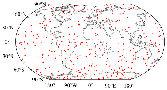
Figure 1.
The spatial distribution of the identified KBR outliers in February 2011.
Additionally, establishing the observation equations for kinematic orbit and range rate measurements necessitates the incorporation of background force models, including both conservative acceleration and non-conservative acceleration components. The non-conservative accelerations can be determined using observations of high-precision accelerometers installed on the GRACE satellites. Table 1 provides an overview of the conservative force models, including N-body perturbations, solid Earth tides, ocean tides, solid Earth pole tides, ocean pole tides, oceanic and atmospheric de-aliasing variations, as well as relativistic corrections.

Table 1.
Dynamic model.
Since Tongji-Acc RL06 is limited to a certain degree and order of 96, we employ the high-precision static gravity field model GOCO06s [45] truncated up to 160 d/o to account for potential influences caused by signals at higher degrees and orders. The N-body disturbances are directly computed based on the gravitational interactions with the sun and the moon [46]. To calculate the precise positions of the sun and the moon, the JPL DE421 planetary Ephemeris [47] is employed. Following the IERS 2010 conventions [48], the impacts of the solid tides and solid pole tides are compensated. To effectively account for the ocean tide effects, we utilized the FES2014b ocean tide model that encompasses 34 primary tidal components [49]. For the secondary ocean tides, the admittance theory proposed by Rieser et al. (2012) is used [50], which conducts linear interpolation based on the primary tides of FES2014b in accordance with the IERS2010 conventions. The perturbation of ocean pole tides is addressed using the Desai model developed by Desai et al. (2002) [51]. In order to remove the non-tidal variations in the atmosphere and ocean, we utilize the Atmospheric and Ocean De-aliasing Level-1B Release 06 product (AOD1B RL06) up to a degree and order of 180, which is provided via the GFZ [52]. Following the IERS2010 conventions, we take the effects of general relativity into account.
4. Results
Using the proposed acceleration method that incorporates the inter-satellite range rate observations, we compute a time series of monthly gravity field models called Tongji-Acc RL06 from GRACE Level-1B RL03 data covering the period from April 2002 to December 2016. In this paper, the quality assessment of Tongji-Acc RL06 monthly models involves a comparative analysis with CSR RL06, GFZ RL06, and JPL RL06 monthly solutions in terms of signal and noise characteristics. In Section 4.1, the comparison is performed in the spectrum domain. The spatial distribution of global mass changes and annual amplitudes is discussed in Section 4.2. To verify the consistency of model signals, an assessment is conducted in Section 4.3 by examining annual amplitudes across river basins with different sizes and analyzing trends and uncertainties in land–ice areas from the four solutions. The root mean squares (RMS) values of mass change residuals over the Sahara Desert and the Karakum Desert are subsequently computed in Section 4.4 to estimate the noise levels of the models.
4.1. Spectrum Analyses
To perform the analyses of signals and noise in the frequency domain, the geoid degree variances of various GRACE monthly gravity field models are calculated with respect to the high-precision static gravity field model GOCO06s. To comprehensively analyze the quality of the derived solutions, we plotted the geoid degree variances (GDV) for three months under varying observational conditions [8] in Figure 2. These three months include January 2003 with early lousy data, April 2003 with repeat orbit cycles, and January 2014 representing the late-year weaker data with gaps. Additionally, the average geoid degree variance (AGDV) over the period from April 2002 to December 2016 is displayed as well.
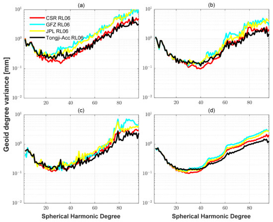
Figure 2.
The geoid degree variances w.r.t GOCO06s: (a) January 2003; (b) April 2003; (c) January 2014; and (d) long-term mean over the period from April 2002 to December 2016.
On one hand, it is widely accepted that the GRACE gravity field solutions are dominated by signals at the lower degrees (approximately before degree 30) [53], resulting in a gradual decrease in amplitudes as the degree increases within this range, as depicted in Figure 2. On the other hand, the higher-degree portions beyond degree 40 primarily represent noise, leading to an amplification of amplitudes with increasing degrees [54,55]. As such, the relatively smaller amplitudes observed at higher-degree ranges generally indicate lower noise in the GRACE models [56]. In Figure 2, it is apparent that the signal level (about below 20 degrees) exhibited by Tongji-Acc RL06 closely aligns with those of other models, demonstrating that the proposed acceleration method can effectively retrieve the gravity field signals from the inter-satellite range rate observations. Nevertheless, Tongji-Acc RL06 generally shows a more significant noise reduction beyond degree 40 in comparison with CSR RL06, GFZ RL06, and JPL RL06. Within the degree range of 20 to 40, Tongji-Acc RL06 generally agrees with GFZ RL06 and JPL RL06, regardless of data quality. The above analyses suggest that the improved acceleration method is able to retain lower-degree gravity field signals as the dynamic method used for developing CSR RL06, GFZ RL06, and JPL RL06. Additionally, it significantly reduces the high-degree noise in gravity field solutions under varying observational conditions.
Since the geoid degree variances solely capture the mean signal and noise for each degree, the differences in the geopotential coefficients between the solutions used in Figure 2 and GOCO06s for each degree and order are further plotted in Figure 3. As depicted in Figure 3, Tongji-Acc RL06 is more effective in determining the above 60-degree zonal (order 0) and near-zonal coefficients than the other three models. Furthermore, notable noise distinctions can be observed among the four solutions at the higher degrees and orders. In general, Tongji-Acc RL06 exhibits a pronounced reduction in noise compared with the other three models at high degrees.
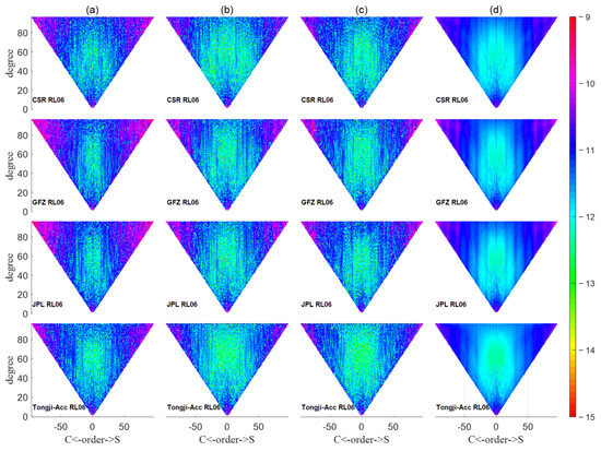
Figure 3.
The differences in geopotential coefficients (log10 scale) w.r.t GOCO06s: (a) January 2003; (b) April 2003; (c) January 2014; and (d) long-term mean for the period from April 2002 to December 2016.
4.2. Global Mass Variation Signal
In consideration of correlated noise and high-frequency noise in the GRACE monthly gravity field solutions [25,42], post-processing filtering methods such as Gaussian smoothing [57], DDK filtering [58], and decorrelation filter [59] have to be used. To mitigate the effects of the correlated noise and high-frequency noise, a 300 km Gaussian smoothing and P4M6 decorrelation filtering technology is employed in this section. Furthermore, the degree-one coefficients of the four gravity field models are replaced with the results from Swenson et al. (2008) [60]. The C20 coefficients of the GRACE models are substituted with the outcomes obtained through Satellite Laser Ranging (SLR) [61].
In this research, the global mass variation signals for Tongji-Acc RL06, CSR RL06, GFZ RL06, and JPL RL06 are extracted with respect to the average solutions from April 2002 to December 2016 in terms of equivalent water height (EWH) grids. Subsequently, the global mass changes in January 2003, April 2003, and January 2014 are displayed in Figure 4, which represent three typical months characterized by varying data quality. The selection of these three months is based on the highly problematic data in January 2003, deep orbit repeat observation during April 2003, and the reduced amount of data in January 2014. In Figure 4, the global mass change signals from Tongji-Acc RL06 demonstrate a good consistency with those from the other three models. All four solutions indicate that strong mass change signals are primarily observed in inland regions, while mass variations in ocean areas exhibit relatively smooth patterns. However, despite the application of 300 km Gaussian smoothing and P4M6 decorrelation filtering, the spatial maps of the four solutions exhibit noticeable striping noise, particularly over mid- and low-latitude regions. One contributing factor to this issue stems from the polar orbital configuration of the GRACE satellites, leading to sparse ground track coverage at the mid- and low-latitudes [55,62]. Furthermore, we can observe that in these three months characterized by inferior data quality, the Tongji-Acc RL06 generally exhibits a lower noise level.
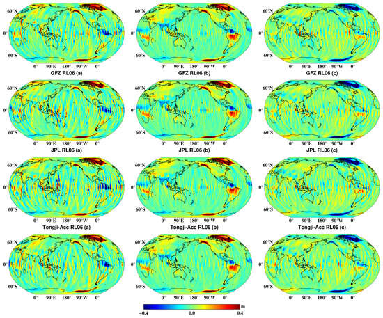
Figure 4.
Monthly global mass changes from the GRACE models processed using 300 km Gaussian smoothing and P4M6 decorrelation filtering: (a) January 2003; (b) April 2003; and (c) January 2014.
The spatial distribution of the estimated annual amplitudes of mass changes for the period from April 2002 to December 2016 is further depicted in Figure 5, showing a good agreement among the four solutions. In general, the four solutions all retrieve the strong annual signals over lands, primarily in the Amazon River Basin, Greenland, Ganges River Basin in India, Qinghai–Tibet Plateau in China, Zambezi River Basin in Africa, and the Mississippi River Basin, as noted by Meyer et al. (2016) [54]. These results suggest a comparable signal level between the Tongji-Acc RL06 and the other three models.
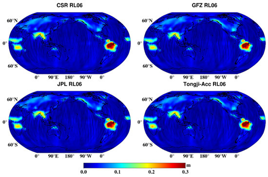
Figure 5.
Annual amplitudes of global mass changes obtained from the four GRACE models processed using 300 km Gaussian smoothing and P4M6 decorrelation filtering.
4.3. Mass Variation Signal in River Basin and Land–Ice Areas
Monthly gravity field solutions have played a crucial role in signal estimates over hydrological and land–ice areas [2,63,64,65,66,67]. In this paper, we have selected ten river basins with varying latitudes and sizes (e.g., Amazon, Tennessee—the smallest sub-basin of the Mississippi River, and Congo River), along with two ice sheets (i.e., Gulf of Alaska and Greenland) for investigation. After applying P4M6 decorrelation filtering and 300 km Gaussian smoothing to the CSR RL06, GFZ RL06, JPL RL06, and Tongji-Acc RL06 solutions, we derived mass change time series for these regions. As shown in Figure 6, there is good consistency among the four solutions, exhibiting pronounced annual amplitudes across these 12 regions. Additionally, both the Gulf of Alaska and Greenland exhibit significant mass loss, which aligns with previous findings by Chen et al. (2011) and Luthcke et al. (2013) [63,68].
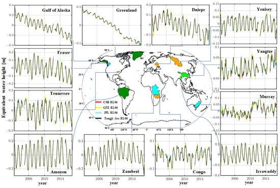
Figure 6.
Time series of mass change from the four GRACE models processed using 300 km Gaussian smoothing and P4M6 decorrelation filtering.
To further evaluate the performance of the four solutions, we computed the mean annual amplitudes for the four solutions using two combined filtering methods (i.e., a P4M6 decorrelation filtering combined with Gaussian smoothing with a radius of 300 km and 500 km, respectively). The corresponding results are presented in Table 2 and Table 3. In Table 2, regardless of the filtering strategies employed, Tongji-Acc RL06 generally exhibits comparable mean annual amplitudes as the other three models. As in previous studies, the annual amplitudes calculated based on the CSR RL06 in the Amazon and Murray River Basins are 20.0 cm and 2.1 cm, respectively, aligning with the findings of this paper [69]. In Table 3, the trend estimates from Tongji-Acc RL06 are in good agreement with those from the other three models as well. Particularly, when using P4M6 decorrelation filtering and 300 km Gaussian smoothing, the trends over the Gulf of Alaska and Greenland are estimated to be −2.9 ± 0.2 cm/year and −6.8 ± 0.3 cm/year for Tongji-Acc RL06, respectively. The result of −6.8 ± 0.3 cm/year for Greenland demonstrates a strong consistency with the trend estimate of −6.7 ± 0.2 cm/year by Zhong et al. (2023) [69].

Table 2.
Mean annual amplitudes from the four GRACE models processed using combined filtering methods over 12 areas for the period from April 2002 to December 2016 (cm).

Table 3.
Trend estimates from the four GRACE models processed using combined filtering methods over Greenland and the Gulf of Alaska for the period from April 2002 to December 2016 (cm/year).
4.4. Noise Levels over the Sahara and Karakum Deserts
Considering the significant noise characteristics in desert areas [70,71], we selected the Sahara Desert and the Karakum Desert as two examples for analyzing the noise in different gravity field solutions. During the noise analysis, a combination of 300 km Gaussian smoothing and P4M6 decorrelation filtering is first applied, which is considered moderate filtering. After removing significant seasonal terms (including bias, trend, acceleration, annual, semi-annual, and S2 seasonal components) [72], the RMS values of the residual mass variations from the four solutions for the period between April 2002 and December 2016 are illustrated in Figure 7. The noise level in Figure 7 is generally lower for Tongji-Acc RL06 compared with CSR RL06, GFZ RL06, and JPL RL06, since the RMS values over both deserts mainly reflect the noise of monthly models [73]. Additionally, Figure 7 exhibits several individual spikes, which are attributed to poor data quality over certain months (e.g., January 2003, January 2004, September 2004, etc.) [8].
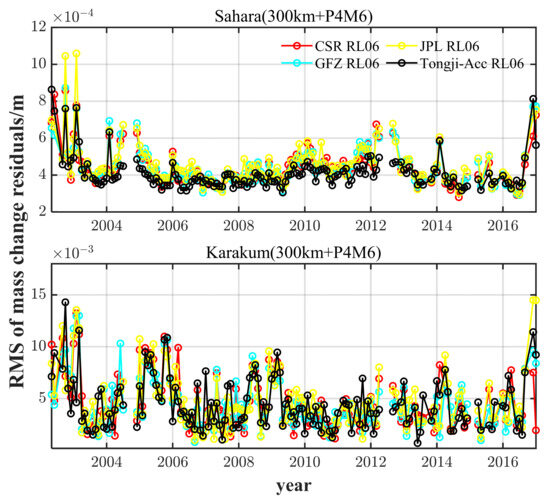
Figure 7.
Time series of RMS values of mass change residuals from the four GRACE models for the period from April 2002 and December 2016 in both deserts.
For a comprehensive evaluation of noise levels for the four solutions under varying filtering strengths, based on P4M6 decorrelation filtering, Table 4 provides statistics on the average RMS of mass change residuals over both deserts at different Gaussian smoothing radii (i.e., 0 km, 100 km, 200 km, 300 km, 400 km, and 500 km). Three key insights can be derived from Table 4: (1) the combination of P4M6 decorrelation filtering and Gaussian smoothing with a larger radius leads to a noticeable decrease in model noise levels; (2) Tongji-Acc RL06 shows a lower noise level compared with the other three models, especially when the smoothing radius is no more than 300 km; however, further increasing the smoothing radius will reduce the difference in noise between Tongji-Acc RL06 and the other models; and (3) particularly in the case of no Gaussian smoothing, Tongji-Acc RL06 demonstrates substantial enhancements in noise reduction compared with CSR RL06. The corresponding noise reductions reach 55.8% and 61.5% over the Sahara Desert and the Karakum Desert, respectively. In general, these findings suggest that the proposed acceleration method is capable of reducing the noise in monthly gravity field solutions.

Table 4.
Mean RMS of mass change residuals from the four GRACE models for the period from April 2002 to December 2016.
Note that the mean RMS only reflects the overall level of model noise. Therefore, we further plot the spatial distribution of RMS values over both deserts in Figure 8 and Figure 9, where a P4M6 decorrelation filtering combined with 300 km Gaussian smoothing is used. We can observe from Figure 8 and Figure 9 that the Tongji-Acc RL06 model demonstrates a spatial distribution characterized by lower RMS values in both desert regions in contrast to the other three models. The finding further supports our conclusion that Tongji-Acc RL06 exhibits reduced noise levels compared with the CSR RL06, GFZ RL06, and JPL RL06, which is consistent with what we conclude from Figure 7.
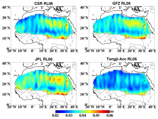
Figure 8.
RMS values of mass change residuals over the Sahara Desert computed from the four GRACE models processed using 300 km Gaussian smoothing and P4M6 decorrelation filtering.
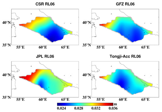
Figure 9.
RMS values of mass change residuals over the Karakum Desert computed from the four GRACE models processed using 300 km Gaussian smoothing and P4M6 decorrelation filtering.
5. Discussion
In the previous sections, we primarily analyzed the signal and noise levels of the GRACE models at different scale regions. Although the signal levels are consistent among the four solutions, distinctions in model quality arise due to the presence of both signal and noise components within each individual GRACE model. To accurately assess the quality of the various GRACE models, a feasible approach involves separating the signal from noise and quantifying their respective signal-to-noise ratios (SNRs). In this paper, we select two large-scale river basins (i.e., Amazon and Zambezi) and another two small-scale river basins (i.e., Tennessee and Irrawaddy) as illustrative examples to analyze the quality of various models. During computing the SNRs for the four solutions under different filtering strengths, a combination of P4M6 decorrelation filtering and Gaussian smoothing with varying radii (i.e., 0 km, 100 km, 200 km, 300 km, 400 km, and 500 km) is applied. By subtracting the dominant signal terms (including the bias, trend, acceleration, annual, semi-annual, and S2 seasonal terms) from the filtered mass changes, we obtain the mean RMS value of mass change residuals. This mean RMS value mainly represents the noise level of the model under consideration [74]. Considering the predominant annual signals in the selected river basins, as depicted in Figure 6, we can regard the estimated annual amplitude (AMP) as a signal level [70]. Subsequently, we can derive the SNR value according to SNR = AMP/RMS [27].
As a result, the SNR values of different solutions processed using P4M6 decorrelation filtering and Gaussian smoothing with varying radii over the four basins are depicted in Figure 10. It shows that Tongji-Acc RL06 consistently exhibits higher SNR values compared with CSR RL06, GFZ RL06, and JPL RL06 across all filtering procedures in the four regions. Additionally, the spatial distribution of the SNR values for the four solutions in the large-scale Amazon and the small-scale Tennessee River Basins are further illustrated in Figure 11 and Figure 12, respectively. In both figures, a combination of P4M6 decorrelation filtering and 300 km Gaussian smoothing is employed. In the spatial domain, Tongji-Acc RL06 has also improved the SNR values over river basins with distinct sizes, as demonstrated by Figure 11 and Figure 12. Consistent results were obtained in the remaining two regions, which are not shown here. Overall, these findings regarding the SNR values confirm the reliability of the monthly solutions derived using the proposed acceleration method.
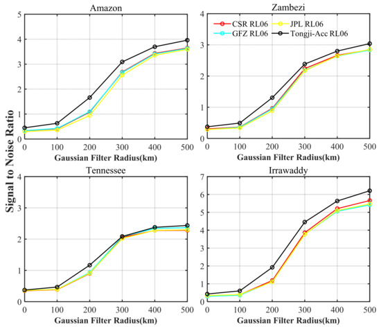
Figure 10.
The SNR values of the four GRACE models processed using a combination of P4M6 decorrelation filtering and Gaussian smoothing with varying radii in four river basins.
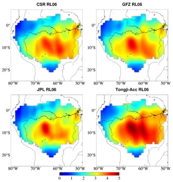
Figure 11.
The SNR values of the four GRACE models processed using P4M6 decorrelation filtering and 300 km Gaussian smoothing in the Amazon River Basin.
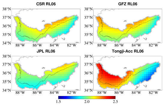
Figure 12.
The SNR values of the four GRACE models processed using P4M6 decorrelation filtering and 300 km Gaussian smoothing in the Tennessee River Basin.
6. Conclusions
In this paper, we propose an improved acceleration approach for utilizing inter-satellite rate measurements during gravity field modeling. Based on the proposed method, a time series of monthly gravity field models complete to a degree and order of 96, referred to as Tongji-Acc RL06, was calculated from inter-satellite range rate and kinematic orbit observations. To evaluate the signal and noise characteristics of Tongji-Acc RL06, we compared geoid degree variances, signal and noise contents in global and local regions with varying sizes, and noise levels over the Sahara Desert and the Karakum Desert.
The resulting geoid degree variances demonstrate a significant agreement between the signal components (below degree 20) of Tongji-Acc RL06 and those of CSR RL06, GFZ RL06, and JPL RL06 models. Nevertheless, Tongji-Acc RL06 exhibits significantly lower noise (above a degree of 40) than the other three models. Following P4M6 decorrelation and 300 km Gaussian smoothing, the global mass variations obtained from Tongji-Acc RL06 exhibit good agreement with those from the other three models. However, regardless of the Gaussian smoothing radius applied, Tongji-Acc RL06 consistently demonstrates a higher SNR across diverse sizes of river basins compared with the other three solutions. Further noise analysis conducted over the Sahara Desert and the Karakum Desert reveals that the noise was significantly reduced in Tongji-Acc RL06. In particular, after applying only the P4M6 decorrelation filtering, Tongji-Acc RL06 achieves a noise reduction of over 55.8% and 61.5% compared with CSR RL06, respectively.
In conclusion, the findings presented in this paper demonstrate that the proposed acceleration approach can effectively extract the gravity field signals from inter-satellite range rate observations comparable to those obtained from the three official models determined using the dynamic method. Nevertheless, the noise of gravity field models has been greatly reduced by the proposed method compared with that of the official models. It is worth noting that a related study by Ray et al. (2009) indicates that the numerical differentiation of range rate yields range acceleration with improved spatial localization characteristics [37]. Based on the GRACE range acceleration data, the resulting C20 estimate obtained using the dynamic method is comparable to that derived from SLR [38]. This study inspires us to further extend the acceleration approach for processing range acceleration data in the future.
Author Contributions
Conceptualization, Q.C.; methodology, Z.S., Q.C. and Y.S.; validation, Z.S., Q.C. and Y.S.; formal analysis, Z.S. and Q.C.; data curation, Q.C.; writing—original draft preparation, Z.S.; writing—review and editing, Q.C. and Y.S. All authors have read and agreed to the published version of the manuscript.
Funding
This work is primarily supported by the National Natural Science Foundation of China (42192532 and 42174099). It also has partial sponsorship from the Fundamental Research Funds for the Central Universities.
Data Availability Statement
Our heartfelt gratitude goes to JPL for generously providing the GRACE Level-1B data, which can be accessed at https://podaac.jpl.nasa.gov/, accessed on 5 June 2023. Additionally, we extend our sincere acknowledgments to the Graz University of Technology for providing the kinematic orbits, available at http://ftp.tugraz.at/outgoing/ITSG/, accessed on 10 June 2023.
Acknowledgments
In this section, we would like to thank Wei Feng for using the GRACE Matlab Toolbox (GRAMAT) to conduct part of the research for this article [75].
Conflicts of Interest
The authors declare no conflict of interest.
Appendix A
Appendix A.1. Overview of Classical Acceleration Method
As provided in Equation (A1), the classical acceleration method utilizes the concept of the 3-point differentiation to establish a functional relationship between the acceleration computed from kinematic orbits at three adjacent epochs and the weighted average acceleration [9,19,22,36]:
in which represents the position vector of the satellite at time t; the sampling interval of observations, denoted as Δt, is set to 5 s; the integration variable is associated with time; and the force acting on the satellite at time consists of both conservative and non-conservative forces.
Since the weight function for an integration arc with epochs defined in Equation (A2) is a high-order polynomial, the computation is exceedingly complicated. To simplify the calculation of the weight function, Chen et al. (2015) applied an -order Cowell integral to directly establish the correlation between the orbits at the three adjacent epochs and the weighted average acceleration, leading to a discrete observation equation for orbits as follows [19]:
where denotes the Cowell integral coefficients; N stands for the maximum number of epochs within the integral arc. In this study, Equation (A3) serves as the basis for establishing the relationship between the geopotential coefficients and the inter-satellite range rate observations. The computation of an n-order Cowell integral involves the preceding n acceleration records since the start of the integration arc. For convenience, observation equations for the previous epochs were ignored in Chen et al.’s study (2015) [19].
Appendix A.2. Improved Acceleration Method
For each epoch within the integral arc, as defined in Equation (A4), the orbit vector can be expressed as a kinematic orbit observation vector plus a correction vector .
By substituting Equation (A4) into Equations (1) and (2), followed by linearization, we can derive the observation equations for the satellite’s orbit positions at the time in the following manner:
Analogously, the linearized orbit observation equations at the time and can be generated as follows:
where and represent the a priori geopotential coefficients and accelerometer parameters, respectively; and are their corresponding corrections.
The substitution of Equation (A4) into Equation (3) is performed, followed by linearization to derive the subsequent equation as follows:
For brevity, the orbit observation Equations (A5) and (A6) for both satellites in the -th arc can be summarized in matrix form as follows:
where and stand for the design matrices regarding the parameter vector to be estimated and the correction vector to kinematic orbits, respectively; the symbols A and B represent GRACE A and GRACE B, separately; and the residual vector is the difference between the kinematic orbit observations and the reference orbit positions computed via numerical integration according to Equations (A5) and (A6).
The relationship between the inter-satellite range rates and the orbital position and velocity vectors of both satellites is established in the following manner.
Inserting Equations (A5)–(A7) into Equation (A9), we derive the linearized observation equation for inter-satellite range rate measurements as follows:
where the reference inter-satellite range rate, denoted as , is directly determined by employing the reference position and velocity vectors of the two GRACE satellites; the term represents the residual of the inter-satellite range rate observation. Similar to Equation (A8), the observation equation for the inter-satellite range rate observations in the -th arc can be rewritten as follows:
where and stand for the design matrices regarding the corrections to kinematic orbit observations of both satellites; the design matrix is the partial derivative matrix with respect to the unknown parameter vector ; is the difference between the range rate observations and the reference value . As demonstrated in Equations (A5) and (A6), the incorporation of the satellite’s initial position and velocity parameters results in orbit observation equations for each satellite in the k-th arc, corresponding to the number of orbit observation epochs. Consequently, both the design matrices and possess characteristics of being full-rank and invertible.
Integrating Equations (A8) and (A11), we can derive more concise observation equations for the kinematic orbit observations of both satellites and the inter-satellite range rate data in the -th arc as follows:
where
In Equations (A12) to (A14), the parameters to be estimated include the geopotential coefficients and local parameters (i.e., the initial position and velocity parameters, as well as accelerometer scales and biases). Subsequently, the following sub-normal Equation (6) in the k-th arc corresponding to Equation (A12) can be easily established through the least squares method.
Note that the unknown parameter vector in the sub-normal Equation (6) in the -th arc consists of the geopotential coefficients and local parameters. To generate the final monthly normal equation only regarding the unknown geopotential coefficients, the local parameters have to be eliminated. For a detailed implementation of the elimination process, one can refer to Beutler et al. (2010b) [44].
References
- Flury, J.; Bettadpur, S.; Tapley, B.D. Precise accelerometry onboard the GRACE gravity field satellite mission. Adv. Space Res. 2008, 42, 1414–1423. [Google Scholar] [CrossRef]
- Tapley, B.D.; Bettadpur, S.; Watkins, M.; Reigber, C. The gravity recovery and climate experiment: Mission overview and early results. Geophys. Res. Lett. 2004, 31, L09607. [Google Scholar] [CrossRef]
- Kornfeld, R.P.; Arnold, B.W.; Gross, M.A.; Dahya, N.T.; Klipstein, W.M.; Gath, P.F.; Bettadpur, S. GRACE-FO: The Gravity Recovery and Climate Experiment Follow-On Mission. J. Spacecr. Rocket. 2019, 56, 931–951. [Google Scholar] [CrossRef]
- Abich, K.; Abramovici, A.; Amparan, B.; Baatzsch, A.; Okihiro, B.B.; Barr, D.C.; Bize, M.P.; Bogan, C.; Braxmaier, C.; Burke, M.J.; et al. In-orbit performance of the GRACE Follow-on laser ranging interferometer. Phys. Rev. Lett. 2019, 123, 031101. [Google Scholar] [CrossRef] [PubMed]
- Bettadpur, S. UTCSR Level-2 Processing Standards Document for Level-2 Product Release 0006, 1–16; Center for Space Research, The University of Texas at Austin: Austin, TX, USA, 2018. [Google Scholar]
- Yuan, D. JPL Level-2 Processing Standards Document for Level-2 Product Release 06, 1–16; Jet Propulsion Laboratory, California Institute of Technology: Pasadena, CA, USA, 2018. [Google Scholar]
- Dahle, C.; Flechtner, F.; Murböck, M.; Michalak, G.; Neumayer, H.; Abrykosov, O.; Reinhold, A.; König, R. GFZ Level-2 Processing Standards Document for Level-2 Product Release 06; GFZ German Research Centre for Geosciences: Potsdam, Germany, 2018. [Google Scholar]
- Kvas, A.; Behzadpour, S.; Ellmer, M.; Klinger, B.; Strasser, S.; Zehentner, N.; Mayer-Gürr, T. ITSG-Grace2018: Overview and evaluation of a new GRACE-only gravity field time series. J. Geophys. Res. Solid Earth. 2019, 124, 9332–9344. [Google Scholar] [CrossRef]
- Liu, X.; Ditmar, P.; Siemes, C.; Slobbe, D.C.; Revtova, E.; Klees, R.; Riva, R.; Zhao, Q. DEOS Mass Transport model (DMT-1) based on GRACE satellite data: Methodology and validation. Geophys. J. Int. 2010, 181, 769–788. [Google Scholar] [CrossRef]
- Han, S.-C.; Shum, C.K.; Bevis, M.; Ji, C.; Kuo1, C.-Y. Crustal dilatation observed by GRACE after the 2004 Sumatra-Andaman earthquake. Science 2006, 313, 658–662. [Google Scholar] [CrossRef]
- Han, S.-C.; Sauber, J.; Riva, R.E.M. Contribution of satellite gravimetry to understanding seismic source processes of the 2011 Tohoku-Oki earthquake. Geophys. Res. Lett. 2011, 38, L24312. [Google Scholar] [CrossRef]
- Wahr, J.; Molenaar, M.; Bryan, F. Time variability of the earths gravity field hydrological and oceanic effects and their possible detection using grace. J. Geophys. Res. Solid Earth 1998, 103, 30205–30229. [Google Scholar] [CrossRef]
- Zhou, J.; Wang, L.; Zhong, X.; Yao, T.; Qi, J.; Wang, Y.; Xue, Y. Quantifying the major drivers for the expanding lakes in the interior Tibetan Plateau. Sci. Bull. 2022, 67, 474–478. [Google Scholar] [CrossRef]
- Yin, L.; Wang, L.; Keim, B.D.; Konsoer, K.; Yin, Z.; Liu, M.; Zheng, W. Spatial and wavelet analysis of precipitation and river discharge during operation of the Three Gorges Dam, China. Ecol. Indic. 2023, 154, 110837. [Google Scholar] [CrossRef]
- Wal, W.V.D.; Wu, P.; Sideris, M.G.; Shum, C.K. Use of GRACE determined secular gravity rates for glacial isostatic adjustment studies in North-America. J. Geodyn. 2008, 46, 144–154. [Google Scholar]
- Gunter, B.C.; Wittwer, T.; Stolk, W.; Klees, R.; Ditmar, P. Comparison of Regional and Global GRACE Gravity Field Models at High Latitudes. In Geodesy for Planet Earth, Proceedings of the 2009 IAG Symposium, Buenos Aires, Argentina, 31 August 31–4 September 2009; Springer: Berlin/Heidelberg, Germany, 2012. [Google Scholar]
- Luthcke, S.B.; Zwally, H.J.; Abdalati, W.; Rowlands, D.D.; Ray, R.D.; Nerem, R.S.; Lemoine, F.G.; McCarthy, J.J.; Chinn, D.S. Recent Greenland ice mass loss by drainage system from satellite gravity observations. Science 2006, 314, 1286–1289. [Google Scholar] [CrossRef] [PubMed]
- Siemes, C.; Ditmar, P.; Riva, R.E.M.; Slobbe, D.C.; Liu, X.L.; Farahani, H.H. Estimation of mass change trends in the Earth’s system on the basis of GRACE satellite data, with application to Greenland. J. Geod. 2013, 87, 69–87. [Google Scholar] [CrossRef]
- Chen, Q.; Shen, Y.; Chen, W.; Zhang, X.; Ju, X. A modified acceleration-based monthly gravity field solution from grace data. Geophys. J. Int. 2015, 202, 1190–1206. [Google Scholar] [CrossRef]
- Ditmar, P.; van Eck van der Sluijs, A.A. A technique for modeling the Earth’s gravity field on the basis of satellite accelerations. J. Geod. 2004, 78, 12–33. [Google Scholar] [CrossRef]
- Ditmar, P.; Kuznetsov, V.; van Eck van der Sluijs, A.A.; Schrama, E.; Klees, R. DEOS_CHAMP-01C_70’: A model of the Earth’s gravity field computed from accelerations of the CHAMP satellite. J. Geod. 2006, 79, 586–601. [Google Scholar] [CrossRef][Green Version]
- Farahani, H.H.; Ditmar, P.; Inácio, P.; Didova, O.; Gunter, B.; Klees, R.; Guo, X.; Guo, J.; Sun, Y.; Liu, X.; et al. A high resolution model of linear trend in mass variations from DMT-2: Added value of accounting for coloured noise in GRACE data. J. Geodyn. 2017, 103, 12–25. [Google Scholar] [CrossRef][Green Version]
- Mayer-Gürr, T. Gravitationsfeldbestimmung aus der Analyse kurzer Bahnbögen am Beispiel der Satellitenmissionen CHAMP und GRACE. Ph.D. Thesis, University of Bonn, Bonn, Germany, 2006. [Google Scholar]
- Mayer-Gürr, T.; Eicker, A.; Ilk, K.H. ITG-Grace02s: A GRACE gravity field derived from range measurements of short arcs. In Gravity Field of the Earth, Proceedings of the 1st International Symposium of the International Gravity Field Service (IGFS), Istanbul, Turkey, 28 August–1 September; Command of Mapp: Ankara, Turkey, 2007; Volume 18, pp. 193–198. [Google Scholar]
- Mayer-Gürr, T.; Zehentner, N.; Klinger, B.; Kvas, A. ITSG-Grace2014: A new GRACE gravity field release computed in Graz. In Proceedings of the Oral Presentation at the GRACE Science Team Meeting, Potsdam, Germany, 29 September 2014. [Google Scholar]
- Chen, Q.; Shen, Y.; Zhang, X.; Chen, W.; Hsu, H. Tongji-GRACE01: A GRACE-only Static Gravity Field Model Recovered from GRACE Level-1B Data using Modified Short Arc Approach. Adv. Space Res. 2015, 56, 941–951. [Google Scholar] [CrossRef]
- Chen, Q.; Shen, Y.; Chen, W.; Francis, O.; Zhang, X.; Chen, Q.; Li, W.; Chen, T. An optimized short-arc approach: Methodology and application to develop refined time series of Tongji-grace2018 GRACE monthly solutions. J. Geophys. Res. Solid Earth 2019, 124, 6010–6038. [Google Scholar] [CrossRef]
- Jekeli, C. The determination of gravitational potential differences from satellite-to-satellite tracking. Celest. Mech. Dyn. Astron. 1999, 75, 85–101. [Google Scholar] [CrossRef]
- Han, S.C. Efficient Global Gravity Field Determination from Satellite-to-Satellite Tracking. Ph.D. Thesis, School of the Ohio State University, Columbus, OH, USA, 2003. [Google Scholar]
- Rummel, R. Gravity Parameter Estimation from Large Data Sets Using Stabilized Integral Formulas and a Numerical Integration Based on Discrete Point Data; Department of Geodetic Science and Surveying, Ohio State University: Columbus, OH, USA, 1982. [Google Scholar]
- Shen, Y.Z. Study of Recovering Gravitational Potential Model from the Ephemerides of CHAMP; The Institute of Geodesy and Geophysics, Chinese Academy of Science: Wuhan, China, 2000. (In Chinese) [Google Scholar]
- Austen, G.; Grafarend, E.W.; Reubelt, T. Analysis of the Earth’s Gravitational Field from Semi-Continuous Ephemeris of a Low Earth Orbiting GPS-Tracked Satellite of Type CHAMP, GRACE or GOCE; Springer: Berlin/Heidelberg, Germany, 2002. [Google Scholar]
- Shen, Y.; Xu, H.; Wu, B. Simulation of recovery of the geopotential model based on inter-satellite acceleration data in the low-low satellite to satellite tracking gravity mission. Chin. J. Geophys. 2005, 48, B07–B11. [Google Scholar] [CrossRef]
- Ning, J.; Zhong, B.; Luo, Z.; Wang, H. Decorrelation filtering method for recovering the Earth’s gravity field based on satellite acceleration. J. Geod. Geoinf. Sci. 2010, 39, 331–337. [Google Scholar]
- Nie, Y.; Shen, Y.; Pail, R.; Chen, Q.; Xiao, Y. Revisiting Force Model Error Modeling in GRACE Gravity Field Recovery. Surv. Geophys. 2022, 43, 1169–1199. [Google Scholar] [CrossRef]
- Liu, X. Global Gravity Field Recovery from Satellite-to-Satellite Tracking Data with the Acceleration Approach. Ph.D. Dissertation, Delft University of Technology, Delft, The Netherlands, 2008. [Google Scholar]
- Ray, R.D.; Luthcke, S.B.; Boy, J.-P. Qualitative comparisons of global ocean tide models by analysis of intersatellite ranging data. J. Geophys. Res. Ocean. 2009, 114. [Google Scholar] [CrossRef]
- Allgeyer, S.; Tregoning, P.; Mcqueen, H.; McClusky, S.C.; Potter, E.-K.; Pfeffer, J.; McGirr, R.; Purcell, A.P.; Herring, T.A.; Montillet, J.-P. ANU GRACE Data Analysis: Orbit Modeling, Regularization and Inter-satellite Range Acceleration Observations. J. Geophys. Res. Solid Earth 2022, 127, e2021JB022489. [Google Scholar] [CrossRef]
- Jørgen, B.-J.; Gutin, G. Theory, Algorithms and Applications; Springer Science & Business Media: Berlin/Heidelberg, Germany, 2002. [Google Scholar]
- Shampine, L.; Gordon, M. Computer Solution of Ordinary Differential Equations, The Initial Value Problem; W.H.Freeman and Company: San Francisco, CA, USA, 1975; Volume 14, pp. 1097–1105. [Google Scholar]
- Cowell, P.H.; Cormmelin, A.C.D. Investigation of the motion of Halley’s comert from 1759 to 1910. Appendix to Greenwich Observation for 1909. Edinburgh 1910, 18, 637–646. [Google Scholar]
- Farahani, H.H.; Ditmar, P.; Klees, R.; Liu, X.; Zhao, Q.; Guo, J. The static gravity field model DGM-1S from GRACE and GOCE data: Computation, validation and an analysis of GOCE mission’s added value. J. Geod. 2013, 87, 843–867. [Google Scholar] [CrossRef]
- Zhao, Q.; Guo, J.; Hu, Z.; Shi, C.; Liu, J.; Cai, H.; Liu, X. GRACE gravity field modeling with an investigation on correlation between nuisance parameters and gravity field coefficients. Adv. Space Res. 2011, 47, 1833–1850. [Google Scholar] [CrossRef]
- Beutler, G.; Jäggi, A.; Mervart, L.; Meyer, U. The celestial mechanics approach: Application to data of the GRACE mission. J. Geod. 2010, 84, 661–681. [Google Scholar] [CrossRef]
- Kvas, A.; Brockmann, J.M.; Krauss, S.; Schubert, T.; Gruber, T.; Meyer, U.; Mayer-Gürr, T.; Schuh, W.-D.; Jäggi, A.; Pail, R. GOCO06s—A satellite-only global gravity field model. Earth Syst. Sci. Data 2021, 13, 99–118. [Google Scholar] [CrossRef]
- Montenbruck, O.; Gill, E. Satellite Orbits: Models, Methods, and Applications; Springer: Berlin/Heidelberg, Germany, 2000. [Google Scholar]
- Folkner, W.M.; Williams, J.G.; Boggs, D.H. The planetary and lunar ephemeris DE 421. IPN Prog. Rep. 2009, 42, 1. [Google Scholar]
- Petit, G.; Luzum, B. IERS Conventions. (No. IERS-TN-36); Bureau International Des Poids et Mesures Sevres: Sèvres, France, 2010. [Google Scholar]
- Carrere, L.; Lyard, F.; Cancet, M.; Guillot, A. FES 2014, a new tidal model on the global ocean with enhanced accuracy in shallow seas and in the Arctic region. In Proceedings of the Egu General Assembly Conference, Vienna, Austria, 12–17 April 2015. [Google Scholar]
- Rieser, D.; Mayer-Gürr, T.; Savcenko, R.; Bosch, W.; Wünsch, J.; Dahle, C.; Flechtner, F. The Ocean Tide Model EOT11a in Spherical Harmonics Representation. Technical Note. 2012. Available online: https://www.tugraz.at/fileadmin/user_upload/Institute/IFG/satgeo/pdf/TN_EOT11a.pdf (accessed on 5 June 2023).
- Desai, S.D. Observing the pole tide with satellite altimetry. J. Geophys. Res. Ocean. 2002, 107, 7-1–7-13. [Google Scholar] [CrossRef]
- Dobslaw, H.; Bergmann-Wolf, I.; Dill, R.; Poropat, L.; Thomas, M.; Dahle, C.; Esselborn, S.; König, R.; Flechtner, F. A new high-resolution model of non-tidal atmosphere and ocean mass variability for de-aliasing of satellite gravity observations: AOD1B RL06. Geophys. J. Int. 2017, 211, 263–269. [Google Scholar] [CrossRef]
- Luthcke, S.B.; Rowlands, D.D.; Lemoine, F.G.; Klosko, S.M.; Chinn DMcCarthy, J.J. Monthly spherical harmonic gravity feldsolutions determined from GRACE inter-satellite range-ratedata alone. Geophys. Res. Lett. 2006, 33, L02402. [Google Scholar] [CrossRef]
- Chen, Q.; Shen, Y.; Francis, O.; Chen, W.; Zhang, X.; Hsu, H. Tongji-Grace02s and Tongji-Grace02k: High-precision static GRACE-only global Earth’s gravity field models derived by refined data processing strategies. J. Geophys. Res. Solid Earth 2018, 123, 6111–6137. [Google Scholar] [CrossRef]
- Meyer, U.; Jäggi, A.; Jean, Y.; Beutler, G. AIUB-RL02: An improved time-series of monthly gravity fields from GRACE data. Geophys. J. Int. 2016, 205, 1196–1207. [Google Scholar] [CrossRef]
- Pie, N.; Bettadpur, S.V.; Tamisiea, M.; Krichman, B.; Save, H.; Poole, S.; Nagel, P.; Kang, Z.; Jacob, G.; Ellmer, M.; et al. Time variable Earth gravity field models from the first spaceborne laser ranging interferometer. J. Geophys. Res. Solid Earth 2021, 126, e2021JB022392. [Google Scholar] [CrossRef]
- Jekeli, C. Alternative Methods to Smooth the Earth’s Gravity Field; Report 327; Department of Geodetic Science and Surveying, Ohio State University: Columbus, OH, USA, 1981. [Google Scholar]
- Kusche, J.; Schmidt, R.; Petrovic, S.; Rietbroek, R. Decorrelated GRACE time-variable gravity solutions by GFZ, and their validation using a hydrological model. J. Geod. 2009, 83, 903–913. [Google Scholar] [CrossRef]
- Chen, J.L.; Wilson, C.R.; Blankenship, D.; Tapley, B.D. Accelerated Antarctic ice loss from satellite gravity measurements. Nat. Geosci. 2009, 2, 859–862. [Google Scholar] [CrossRef]
- Swenson, S.; Chambers, D.; Wahr, J. Estimating geocenter variations from a combination of GRACE and ocean model output. J. Geophys. Res. 2008, 113, B08410. [Google Scholar] [CrossRef]
- Cheng, M.K.; Tapley, B.D. Variations in the Earth’s oblateness during the past 28 years. J. Geophys. Res. 2004, 109, B09402. [Google Scholar] [CrossRef]
- Dobslaw, H.; Bergmann-Wolf, I.; Forootan, E.; Dahle, C.; Mayer-Gürr, T.; Kusche, J.; Flechtner, F. Modeling of present-day atmosphere and ocean non-tidal de-aliasing errors for future gravity mission simulations. J. Geod. 2016, 90, 423–436. [Google Scholar] [CrossRef]
- Chen, J.L.; Wilson, C.R.; Tapley, B.D. Interannual variability of Greenland ice losses from satellite gravimetry. J. Geophys. Res. 2011, 116. [Google Scholar] [CrossRef]
- Sang, L.; Zhu, G.; Xu, Y.; Sun, Z.; Zhang, Z.; Tong, H. Effects of Agricultural Large-And Medium-Sized Reservoirs on Hydrologic Processes in the Arid Shiyang River Basin, Northwest China. Water Resour. Res. 2023, 59, e2022WR033519. [Google Scholar] [CrossRef]
- Li, Y.; Mi, W.; Ji, L.; He, Q.; Yang, P.; Xie, S.; Bi, Y. Urbanization and agriculture intensification jointly enlarge the spatial inequality of river water quality. Sci. Total Environ. 2023, 878, 162559. [Google Scholar] [CrossRef] [PubMed]
- Liu, Z.; Xu, J.; Liu, M.; Yin, Z.; Liu, X.; Yin, L.; Zheng, W. Remote sensing and geostatistics in urban water-resource monitoring: A review. Mar. Freshw. Res. 2023. [Google Scholar] [CrossRef]
- Mohamed, A.; Abdelrady, A.; Alarifi, S.S.; Othman, A. Geophysical and Remote Sensing Assessment of Chad’s Groundwater Resources. Remote Sens. 2023, 15, 560. [Google Scholar] [CrossRef]
- Luthcke, S.B.; Sabaka, T.J.; Loomis, B.D.; Arendt, A.A.; McCarthy, J.J.; Antarctica, J.C. Greenland and Gulf of Alaska land-ice evolution from an iterated GRACE global mascon solution. J. Glaciol. 2013, 59, 613–631. [Google Scholar] [CrossRef]
- Zhong, B.; Li, X.; Chen, J.; Li, Q. WHU-GRACE-GPD01s: A series of constrained monthly gravity field solutions derived from GRACE-based geopotential differences. Earth Space Sci. 2023, 10, e2022EA002699. [Google Scholar] [CrossRef]
- Kurtenbach, E.; Mayer-Gürr, T.; Eicker, A. Deriving daily snapshots of the Earth’s gravity field from GRACE L1B data using Kalman filtering. Geophys. Res. Lett. 2009, 36. [Google Scholar] [CrossRef]
- Chen, Q.; Shen, Y.; Chen, W.; Zhang, X.; Hsu, H. An improved GRACE monthly gravity field solution by modeling the non-conservative acceleration and attitude observation errors. J. Geod. 2016, 90, 503–523. [Google Scholar] [CrossRef]
- Wahr, J.; Swenson, S.; Zlotnicki, V.; Velicogna, I. Time-variable gravity from GRACE: First results. Geophys. Res. Lett. 2004, 31, 293–317. [Google Scholar] [CrossRef]
- Bonin, J.A.; Bettadpur, S.; Tapley, B.D. High-frequency signal and noise estimates of CSR GRACE RL04. J. Geod. 2012, 86, 1165–1177. [Google Scholar] [CrossRef]
- Chen, J.; Li, J.; Zhang, Z.; Ni, S. Long-term groundwater variations in Northwest India from satellite gravity measurements. Glob. Planet. Change 2014, 116, 130–138. [Google Scholar] [CrossRef]
- Feng, W. GRAMAT: A comprehensive Matlab toolbox for estimating global mass variations from GRACE satellite data. Earth Sci. Inform. 2018, 12, 389–404. [Google Scholar] [CrossRef]
Disclaimer/Publisher’s Note: The statements, opinions and data contained in all publications are solely those of the individual author(s) and contributor(s) and not of MDPI and/or the editor(s). MDPI and/or the editor(s) disclaim responsibility for any injury to people or property resulting from any ideas, methods, instructions or products referred to in the content. |
© 2023 by the authors. Licensee MDPI, Basel, Switzerland. This article is an open access article distributed under the terms and conditions of the Creative Commons Attribution (CC BY) license (https://creativecommons.org/licenses/by/4.0/).