Abstract
Semantic segmentation of point clouds provided by airborne LiDAR survey in urban scenes is a great challenge. This is due to the fact that point clouds at boundaries of different types of objects are easy to be mixed and have geometric spatial similarity. In addition, the 3D descriptions of the same type of objects have different scales. To address above problems, a fusion attention convolutional network (SMAnet) was proposed in this study. The fusion attention module includes a self-attention module (SAM) and multi-head attention module (MAM). The SAM can capture feature information according to correlation of adjacent point cloud and it can distinguish the mixed point clouds with similar geometric features effectively. The MAM strengthens connections among point clouds according to different subspace features, which is beneficial for distinguishing point clouds at different scales. In feature extraction, lightweight multi-scale feature extraction layers are used to effectively utilize local information of different neighbor fields. Additionally, in order to solve the feature externalization problem and expand the network receptive field, the SoftMax-stochastic pooling (SSP) algorithm is proposed to extract global features. The ISPRS 3D Semantic Labeling Contest dataset was chosen in this study for point cloud segmentation experimentation. Results showed that the overall accuracy and average F1-score of SMAnet reach 85.7% and 75.1%, respectively. It is therefore superior to common algorithms at present. The proposed model also achieved good results on the GML(B) dataset, which proves that the model has good generalization ability.
1. Introduction
Airborne LiDAR point clouds, scanned by light detection and ranging equipment mounted on aerial platforms, are a collection of points with original geometric properties. With the rapid development of computer vision and remote sensing technology, the application of airborne LiDAR point cloud data to urban scenes is paid more and more attention, especially in the fields of navigational positioning, automatic driving, smart city, and 3D vision [1], etc. Point clouds in urban scenes are important information carriers, which are consisted of complex surface features. In order to accurately understand 3D urban scenes from the point level, the concept of point cloud semantic segmentation was proposed. Semantic segmentation, as an important technique for LiDAR point cloud data processing, is aimed at subdividing point clouds into several specific point sets with independent attributes, recognizing the target types of point sets, and making semantic marking [2]. Semantic segmentation of airborne LiDAR point clouds in urban scene can quickly extract typical feature information and understand complex urban scenes, so as to effectively reflect the spatial layout, development scale and greening level of the city, which has a crucial role in the fields of urban development planning, smart city and geo-database [3]. Nevertheless, semantic segmentation of point clouds is a great challenge since airborne LiDAR point clouds have characteristics of high redundancy, incompleteness and complexity [4,5].
To extract surface features from 3D point clouds, traditional methods usually construct the corresponding segmentation model according to geometric attributes and data statistical features chosen manually, such as support vector machine (SVM) [6], random forest (RF) [7], conditional random field (CRF) [8], Markov random field (MRF) [9], etc. However, selection of statistical features mainly relies on priori knowledge of operators, which has great randomness, limited ability in feature extraction of point clouds, and poor generalization. With the improvement of calculation power of computers and continuous emerging of 3D scene dataset, deep learning is taking a dominant role in the field of point cloud semantic segmentation field.
Deep learning [10] firstly was used for semantic segmentation of point clouds through rasterization of point clouds. Su et al. [11] proposed Multi-View Convolutional Neural Network (MVCNN), which got the segmentation results through convolution and aggregation of 2D images of point clouds under different perspectives. According to existing snapshots, Boulch et al. [12] produced pairs of snapshots which contained RGB views and depth maps of geometric features, then provided labels for corresponding pixels of each pair of snapshots, and then mapped the marked pixels onto the original data. Wu et al. [13] extracted features from projected 2D images by using CNN, output the pixel-by-pixel labeling chart, refined it with the conditional random field (CRF) model, and finally got the instance-level labels through the traditional clustering algorithm. Besides, voxelization of irregular 3D point clouds is a common method that researchers are used to process the original point clouds. Maturana et al. [14] proposed VoxNet network based on voxelization of point clouds, which classified point clouds by using the supervised 3D convolutional neutral network (CNN). Tchapmi et al. [15] generated the bold voxel labels through the 3D fully convolutional neural network based on voxelization of point clouds and then enhanced the prediction results by combining the trilinear interpolation and fully-connected CRF learning fine granularity. Wang et al. [16] implemented multi-scale voxelization of point clouds and extracts features, made adaptive learning of local geometric features, and realized global optimization of prediction class probabilities by using CRF with full considerations to spatial consistency of point clouds. The above semantic segmentation methods based on multi-views or voxels solve the structural problems and have some practicability. However, semantic segmentation methods based on multi-views are inevitable to lose 3D space information in the rasterization process of point clouds. The semantic segmentation methods based on voxels increase the spatial complexity and incur great expenses for storage and operation.
Therefore, some effective frameworks for direct processing of point cloud data are proposed. Qi et al. [17] designed PointNet, which made pointwise coding through multilayer perception (Mlp) and got global features through aggregation function. Nevertheless, it ignores the concept of local space and lacks extraction and utilization of local features. Qi et al. [18] proposed the improved version of PointNet, denoted as PointNet++. It proposes the density adaptive cut-in layer, learns features of point sets at different scales according to multi-layer sampling and grouping, and captures local detail information. However, PointNet++ still processes each point independently, without considerations to connections among neighbor points. In PointNet++, K nearest neighbor searching results have a problem of single direction. Jiang et al. [19] designed a scale perception descriptor for ordered coding of information from different directions and effective capture of local information of point clouds. Based on KNN construction of local neighbor graph, Wang et al. [20] used EdgeConv module to capture local geometric features of point clouds and learn features by making full use of point neighborhood information. Based on the local neighborhood processing of PointNet++, Zhao et al. [21] increased the adaptive feature adjustment module to transform and aggregate upper and bottom information, then integrated information of different channels through Mlp and max pooling, and strengthened the description ability of features to local neighborhood. Xie et al. [22] proposed selection, aggregation, and transformation of key components by building shape context kernels, captured and spread local and global information to express internal attributes of object points. The transformation component is configured according to the overall network of PointNet. Landrieu et al. [23] divided point clouds into several super-points according to geometric shapes, and then learnt features at each super-point by using the sharing PointNet, thus enabling to predict semantic labels. Li et al. [24] proposed the X-Conv operator based on the spatial local correlation of point cloud data. The X-Conv operator standardizes the disordered point clouds through weighting and replacement of input points, and then extracts local features by using CNN. Based on the SA module of PointNet++, Qian et al. [25] introduced in the InvResMLP module to realize the high-efficiency and practical scaling of model, which solved the problem of gradient disappearance and improves ability of feature extraction. Hua et al. [26] determined features of each point through the pointwise convolution and thereby realized semantic segmentation. Hu et al. [27] replaced farthest point sampling (FPS) of PointNet++ by the random sampling and increased the perception field of each 3D point gradually through the local feature aggregation module, thus retaining the geometric details effectively. Nong et al. [28] performed densely connected the point pairs based on PointNet++, supplemented center point features to learn contextual information, and proposed an interpolation method with adaptive elevation weights to propagate point features. However, the method is limited by the lack of global information connection. Due to the great success of the transformer model [29] in capturing contextual information, researchers have introduced it into 3D point cloud processing [30]. Li et al. [31] proposed geometry-aware convolution to handle a large number of geometric instances, and then supplemented the receptive field with dense hierarchical architecture, and designed an elevation-attention module to improve the classification refinement. Zhao et al. [32] used the transformer to exchange local feature information and fit geometric spatial layout. Guo et al. [33] proposed the offset-attention module to better understand point clouds features and capture local geometric information using neighbor embedding strategy. Zhang et al. [34] introduced a bias based on the transformer model to extract relationships between local points to address the sparsity of point cloud data, and proposed a standardization set abstraction module to extract global information to complement topological relationships.
Although the above methods have achieved some progresses in semantic segmentation of point clouds, they have not adequately considered relations among point features and lack of deep interaction relations. The semantic segmentation of urban LiDAR point clouds is a challenge due to the uneven spatial data distribution of airborne laser point clouds, mixed distribution of point clouds at neighborhood surface boundary, and different scales of the objects with the same semantics. To address these problems, a convolutional network based on fusion attention mechanism which is used for 3D point clouds directly was designed in this study on the basis of PointNet++, which was called as SMAnet. Fusion attention mechanism makes parallel treatment based on self-attention mechanism (SAM) [35] and multi-head attention mechanism (MAM) [29]. The essence of SAM is to calculate similarity according to global features of each point and allocate different weights. With full considerations to interaction among points, the SAM can distinguish the mixed point clouds at surface boundary effectively. With considerations to influences of correlations of different local features on points, the multi-head attention module (MAM) was introduced in. The specific idea behind MAM is to divide high-dimensional features of points into different feature subspaces which contain different attribute information of points. Later, it judges feature similarity among different feature subspaces, thus adjusting subspace channel information. The MAM captures connections among different aspects of point features, makes full use of information correlation in local features, increases fine granularity of network, and can recognize surface points at different scales effectively.
The network also uses the light multi-scale feature extraction and supplements local geometric information by local features at different levels. Moreover, different from previous global feature extraction based on aggregation function, a global information extraction method based on SoftMax-stochastic pooling (SSP) was designed, which expanded the receptive field of network model and increases calculation efficiency as well as segmentation accuracy.
The remainder of this study is organized as follows. Section 2 introduces the proposed SMAnet method and principle. Section 3 introduces the experiment details and experimental results. Section 4 presents the discussion including comparative analysis, ablation experiments and some other additional experiments. Section 5 summarizes experimental conclusions.
2. Methods
2.1. Introduction to the Network Structure
The overall framework of the proposed SMAnet is shown in Figure 1. It covers five modules, namely, data preprocessing layer, feature extraction layer, fusion attention layer, SSP aggregation layer and feature propagation upsampling layer. Each module is introduced as follows:
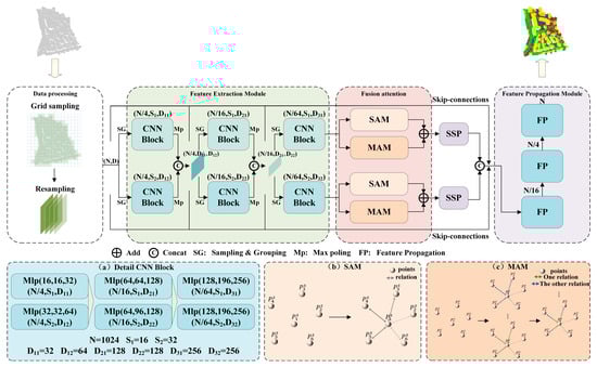
Figure 1.
Framework of SMAnet model.
- (1)
- Firstly, the original data were preprocessed by the grid sampling strategy with considerations to uneven distribution and density of urban LiDAR point clouds, thus getting the standardized massive point cloud dataset as the input of the feature extraction layer. The framework takes the description of point clouds in a zone (denoted as (N, D)) for example, where N is the number of points in the zone and D is the number of point cloud features.
- (2)
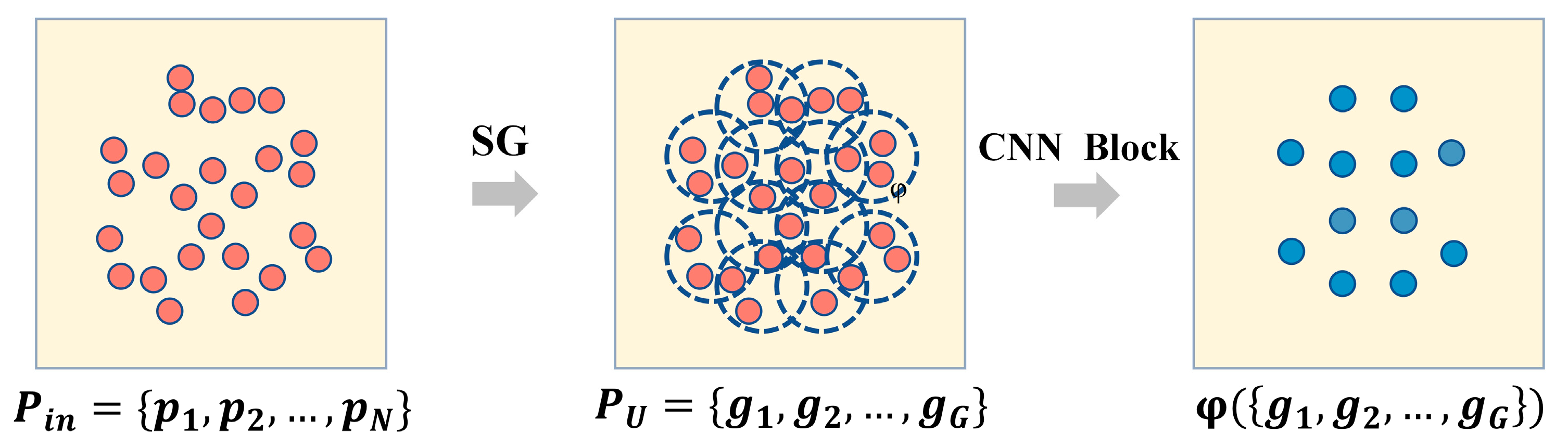
- The attribute features of original point clouds cannot be classified and the original features have to be mapped into a high-dimensional space to learn the high-level semantic information. The feature extraction layer learns features of point clouds by the multi-scale and multi-level method, and it contains the sampling and grouping (SG) and CNN Block. The SG layer firstly makes uniform sampling of input point clouds and the sampling points are used as centroids. Later, the input point clouds are divided into point cloud sets of different scales according to number of points searched within different radii. The numbers of sampling centroids at three layers are N/4, N/16, and N/64, respectively. The numbers of searched points at different scales are denoted as S1 and S2. Finally, multilayer perception (Mlp) is used in CNN Block to extract features of point set in the local neighborhood. The output channel parameters of Mlp and output features of each block are shown in Figure 1a. Different from the complicated structure of PointNet++ feature extraction layer, the proposed SMAnet model applies three-layer feature extraction and takes calculation efficiency and segmentation accuracy of the model into account.
- (3)
- To address insufficient interaction information of point clouds in PointNet++, the fusion attention layer was designed after the feature extraction layer. High-dimensional feature information was strengthened by integration SAM and MAM. The basic principle is shown in Figure 1b,c. The color intensity of segments between two points represents the strength of relations and associations of multiple aspects are expressed by combination of different colors. Some points are given, where is the middle point. The SAM module adds the connection between each point and the central point through global features. In other words, a thrust was applied on the point cloud feature space to push surrounding points of feature deviation to and establish the relationship between surrounding points and . Based on the diversity principle of point cloud, the MAM module explores the deep association among point cloud features in feature spaces according to correlations among different subspace features. Essentially, it applies several different forces onto to establish multiple aspects of relations with surrounding points and associations of point clouds are simulated from different perspectives. The fusion attention layer establishes associations among points from two aspects, thus improving of semantic segmentation accuracy of point clouds.
- (4)
- For giving high-dimensional features of attention, max pooling will lose many important features and it cannot extract global information effectively. Hence, a new aggregation function of SSP was designed as the pooling layer and point cloud features with complicated information were aggregated selectively according to probability after smoothing of SoftMax function to extract global features and filter redundant information.
- (5)
- The feature spreading upsampling layer and feature extraction layer both contain three layers, respectively. Features of all input points were retrieved through skip connections between the learned features and the features from the corresponding feature extraction layer. Finally, pointwise classification was carried out according to features, thus getting the semantic segmentation results.
2.2. Data Preprocessing
Since the urban airborne LiDAR point clouds are sparse and uneven, pre-processing of the raw point cloud data is required. To protect completeness of surface features as much as possible and decrease influences of surface feature size on classification accuracy, we adopted the grid sampling strategy to assure quality of input data and amplify the limited data size [36].
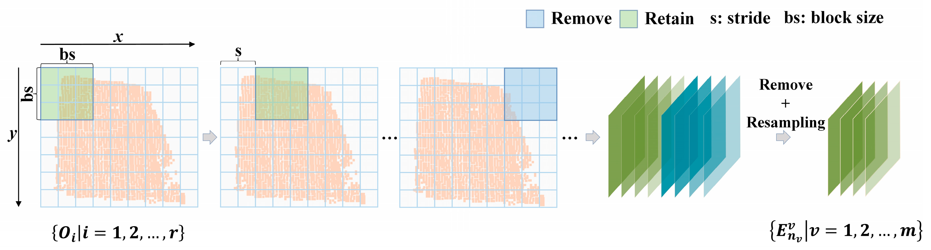
It can be seen from Figure 2 that given a 3D ALS point cloud set with r disordered points , , where d = 6, indicating that each point contains six features, including coordinate data of point (x, y, z), laser scanning intensity, return number, number of returns. To build the training set, the maximum and minimum coordinates along x and y were extracted from the training set, and the length and width of the whole dataset block were calculated. For grid transformation the whole block, points in each grid were determined. According to the preset sampling window size (bs) and the movement step length (s), the whole grid region was retrieved by moving, where the step length was smaller than or equal to the block size. Blocks with points less than half of the preset number of sampling points were deleted. In Figure 2, the blue blocks are deleted ones and the green blocks are the retained ones. The test set was built is the same way. The sliding step length of the test set is equal to the window size and blocks without sufficient points were not deleted. In the training process, it needs enough data for feedforward, feedback, and weight updating of the deep network. To assure that weights of each training of the deep network can be propagated very well, it has to guarantee consistency in number of point clouds of each block. Hence, resampling of points in the block is needed by using Bootstrap sampling method to complete resampling of each block in the dataset. The resampling dataset of blocks was recorded as , where is the set where has nc points in the block v and nc is the fixed number. Finally, the min-max normalization [37] was performed to coordinates of point (x, y, z) and laser intensity. The normalization formula is expressed as Equation (1):
where F can be viewed as the feature that data have to be normalized and , where j = 4. Fmax is the maximum value of the feature and Fmin is the minimum value of the feature.

Figure 2.
Grid sampling.
2.3. Feature Extraction
For semantic segmentation of point clouds, the original attribute features of point cloud data along are far insufficient. It has to learn point features of deeper layers to explore internal attributes of each point. In this study, points were aggregated into groups of different layers by using the feature extraction module and multi-scale features were extracted step by step. It is the first part of the SMAnet. The feature extraction process of each layer is shown in Figure 3. The input data are the data set which is gained from normalization of output results (E) of data preprocessing, that is, the input point data , where is the matrix, N is the quantity of points, and D is features of point. In SG module, we firstly implemented the farthest point sampling [38] ofto determine the centroids of uniform distribution. Groups were then constructed through ball query (BQ) [18] through these centroids. The constructed groups were recorded as , where are the set of group sampling gained by each centroid, , G is the number of groups (that is, the number of centroids of the farthest point sampling) and S represents the number of sampling points based on each centroid.
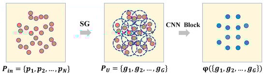
Figure 3.
Feature extraction module.
Local feature extraction was performed to each centroid group () gained after SG sampling and grouping. PU which was gained in the above text was input into the CNN Block module and convolution, BN [39] batch normalization and ReLU [40] nonlinear activation functional operation were performed based on multilayer perception (Mlp) as Equation (2):
In this study, neighborhood aggregation of centroids was carried out according to multilayer structure based on different radii. Moreover, features on different scales were combined. This process can determine local features of different scales well and supplement contextual information.
2.4. Fusion Attention Mechanism
2.4.1. Self Attention Module (SAM)
Urban airborne LiDAR point clouds are complex and diverse. During semantic segmentation of point cloud data in urban scenes, points of adjacent surface categories are easy to be confused (especially at the connection among different surface features). It can be seen from Figure 4a,b that the point clouds of this block are relatively complicated and cover several types of surface features. Point clouds of adjacent surface features were mixed and difficult to be distinguished effectively. As shown in the green circle in the figure, in one case there are roofs and trees which have height feature similarity, and in the other case there are neighbouring shrubs and facades. These adjacent point clouds of different surface objects with similar features are often classified wrongly. Although multi-scale features gained from multilayer learning can supplement local features very well and high-level expression of point clouds can be gained, the information utilization is low and classification has poor precision due to lack of associations among features. To address these problems, the SAM module was introduced into the model. This module allocates different weights to point cloud features according to their associations, thus establishing relations among global features. This improvement strengthens inner links among high-dimensional features of points, and effectively solves the problem that points in adjacent regions of different surface features are difficult to be distinguished.
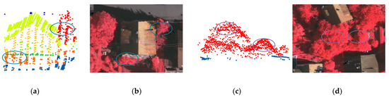
Figure 4.
(a) is mixed region of buildings, shrubs and tree points, Tree points in region (c) have different scales, (b–d) are colour images of the corresponding regions of (a–c).
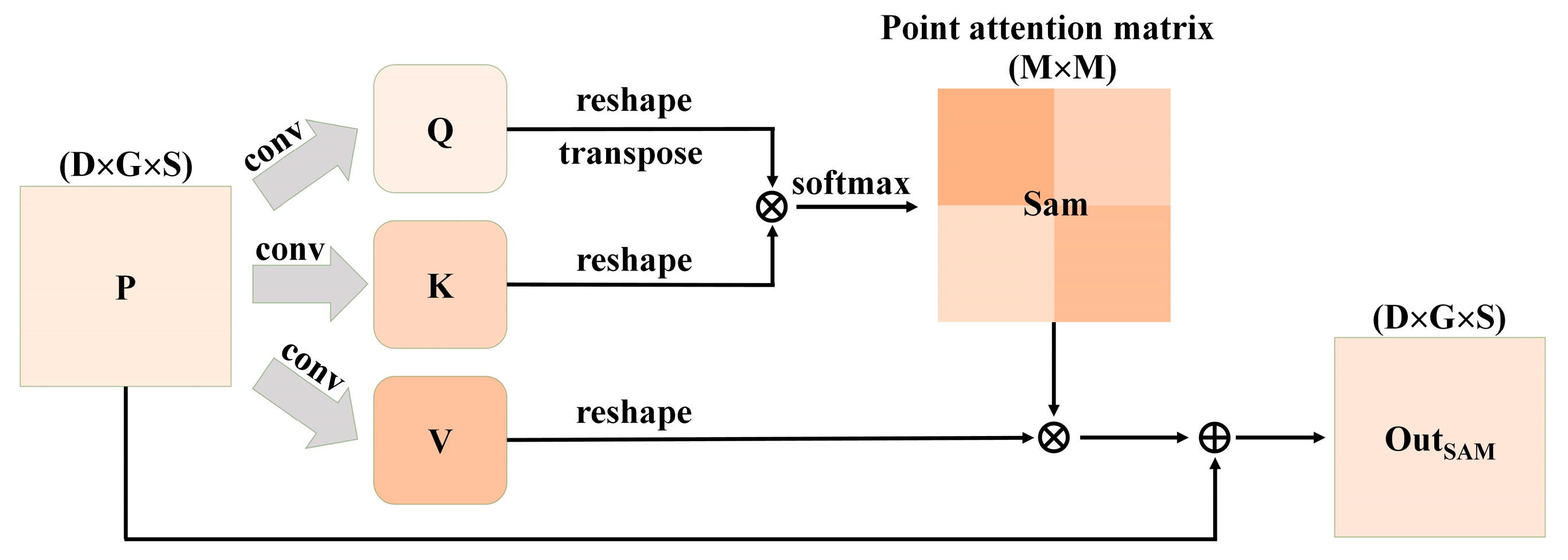
The specific operation of SAM module is shown in Figure 5. after feature extraction was used as input, which was recorded as . It was input into the convolutional layer with D output channels, getting two new feature mapping and . After reshaping of Q and K, and were acquired, where M = G × S, representing quantity of point clouds. The calculation formula of self-attention matrix (Sam) is expressed as Equation (3), where .
where b and e are the positions of the features. is point feature at the appoint position of row b, column e. Specifically, b = 1, 2, …, M and e = 1, 2, …, M. refers to influences of b-th feature on e-th feature, . The attention score matrix is essentially calculated from dot product and SoftMax function. Two features with the higher similarity also have the stronger association. k is the number of channels with a key value of K. For great feature values, in Equation (3) increases significantly. To prevent partial derivative approaching to 0 due to excessive input value of SoftMax [41], such effect is offset by dividing by [29].
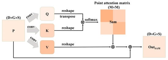
Figure 5.
Operation process of SAM module.
Moreover, the input feature P was input into a convolutional layer with D channels to generate new feature mapping . It was reshaped as . Subsequently, the matrixes of V and the transposition of Sam were multiplied and the result dimensional shape was adjusted as . Finally, it was multiplied with the scale parameter α and calculate sum of elements with original data P. The feature matrixes with associations were output:
where α is a learnable parameter and it is initialized as 0. It makes the network firstly rely on feature information at the current position and then learn long-distance information slowly. P is the original input data and it makes the ultimately generated features have global context information. The SAM module aims to adjust the feature information for each point by allocating weights to the overall features of the point. This treatment established global dependences among different features, so that the network is beneficial for classification of point clouds in the mixing region.
2.4.2. Multi-Head Attention Module (MAM)
Similar with “the same object with different spectra” in remote-sensing images, there’s also a phenomenon of “the same object with different structures” in LiDAR point clouds, especially for point clouds of trees. It can be seen from Figure 4c,d that point clouds of two trees in the oval region have different heights and geometric structures. Due to uneven scale of point clouds of the same surface feature, the point clouds of trees are often wrongly classified as other point clouds. Although SAM can use global information effectively, it will pay attention to its position excessively during coding of information of the current position [42], but uses feature information of other positions insufficiently, thus resulting in information deviation. This is disadvantageous for point cloud classification of surface features with complicated structures. In fact, local features of each point in a complicated feature space are corresponding to diversity attribute of the point. Hence, associations of several features from different aspects in the deep feature space have to be captured fully to establish associations among different points to extract effective information better. To make full use of associations among local features of points, the model is expected to learn different behaviors and capture dependences among different attributes in the feature subspaces based on local features. In this study, the MAM was introduced into processing of point cloud data. It uses query, key, and value (QKV) together in different subspaces to supplement semantic associations among different points, thus strengthening associations in point cloud deeply. This is beneficial for classification of the same category of point clouds with different scales.
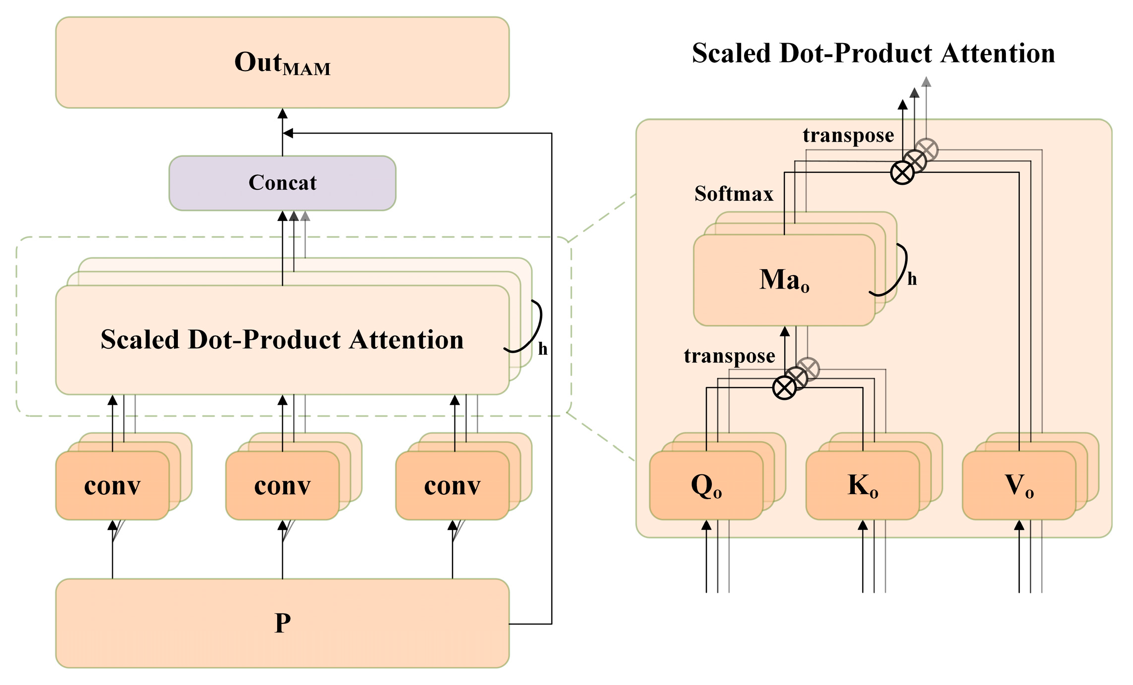
The specific process of MAM is shown in Figure 6. The input data were input into several convolutional layers with D channels and the channels were divided into h heads, getting feature mapping of different subspaces , and . Specifically, , where and . The calculation formula of feature mapping of each subspace is:
where , . Subsequently, the mapped features , and were reshaped into , and . Next, they were input into the scaled dot-product attention module to adjust feature channel information of different subspaces. The process of the scaled dot-product attention module is similar with that of SAM. By calculating the subspace attention , , different subspace feature matrix after enhancement () was finally calculated. The specific calculation process is:
where means to establish the associated feature matrix in each subspace, , and l is the number of channels of Ko. Later, each subspace feature was combined together and then multiplied with the learning parameter (β), followed by adding the original data (P) to supplement information. Finally, the feature matrix () with associations of several features was output, as shown in Equation (7).
where β is initialized as 0 and Concat expresses combination of features. The main purpose of MAM is to learn features and optimize different features of each input data by establishing different subspace attention mechanism according to multiple sets of QKVs, thus balancing possible deviations of SAM. As a result, the semantic features of point clouds have more diversified expressions and the model effect is improved better.
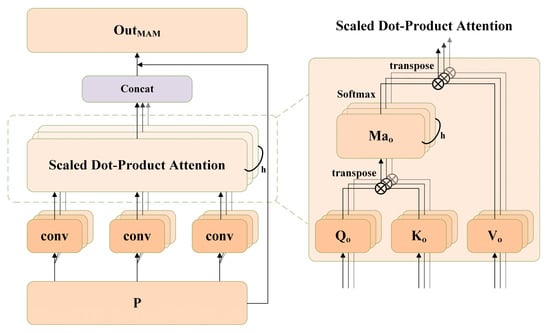
Figure 6.
Operation process of MAM.
Point features extracted by multiple processes belong to high-dimensional spatial features and they contain a lot of information, all of which have their own positions and internal attributes. For better understanding and simulating the complicated interaction relationship among different points, associations of features of discrete points were established from two aspects. On one hand, the SAM analyzes global features of points and supplements the key information of global associations among points from the perspective of global features. On the other hand, the MAM interprets deep connections among discrete points from different feature spaces according to the philosophy that point features are diversified, and it considers association among discrete points more comprehensively. Additionally, the semantic information of point clouds was strengthened by the strategy of parallel SAM and MAM. In other words, association information extracted by SAM and MAM was integrated, which not only can reflect global information association, but also can reflect fusion attention feature matrix of local information associations. Subsequently, global features are extracted through aggregation function. Dimensions of features are decreased and redundant information is reduced. Finally, fusion attention feature matrixes at different scales were combined to supplement the context information.
2.5. SSP Aggregation Algorithm
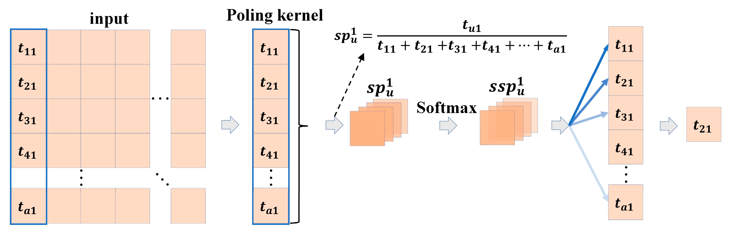
After associations of features are established based on fusion attention mechanism, it has to extract global information from points with close feature associations by using aggregation function. In PointNet++, the global features are extracted through max pooling (MP) [43]. By selecting the maximum value in the pooling region through MP, the texture information can be well learnt, which has the advantage of high-efficiency memory. However, the MP is weak in information retaining and it is easy to lose key information. To explore information of deep point clouds, stochastic pooling [44] was introduced in to process point features. Stochastic pooling calculates probability in feature spaces by using the pooling window with a fixed size and chooses features randomly according to probability, which is conducive to extract information of point cloud spaces. However, extreme situations in feature spaces, for example, negative features are all 0 during function activation based on ReLU, may disturb feature information, thus bringing significant deviations in probability. As a result, it cannot extract effective information accurately. Moreover, it may lose some information upon great fluctuation of the probability space, which is also against extraction of global features. Hence, SoftMax-stochastic pooling (SSP) was designed in this study based on stochastic pooling. Essentially, the SSP normalizes probability through SoftMax function and implements smoothing the feature probability space. This aggregation function makes more information to be used, expands the receptive field of the network, and increases the information acquisition ability of the model.
The SSP aggregation algorithm is shown in Figure 7. For the input feature I, probability of each group was calculated under the fixed pooling kernel. Take the first group for example. The probability was denoted as {}, where is the probability set of the first column, and a is the quantity of features in each column. This probability is the proportion of feature values of each position in all feature values of the group. Next, smoothing of probability of each group was carried out based on SoftMax, thus getting the relatively gentle probability set {}. Finally, extraction of features is carried based on processed probabilities. The SSP algorithm is realized through average pooling and K-nearest neighbor sampling [38], as shown in Equations (8) and (9).
where I is the output of the fusion attention module, AP refers to average pooling, refers to the nearest neighbor interpolation, means the number of K-nearest neighbor samples, and expresses probability-based sampling. The SSP algorithm can prevent overfitting of the model effectively, increase perception field of features, and deepen fine granularity of the network.
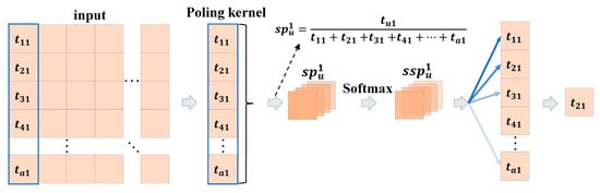
Figure 7.
SSP aggregation algorithm.
2.6. Upsampling and Semantic Segmentation
Downsampling was applied in the feature extraction layer. Although it can guarantee the acquisition of global information, it may fail to complete the segmentation task due to the decrease of points. To assure the same numbers between input and output points of the model, the adjacent point features were chosen for interpolation and features were propagated from subsampling point clouds to the denser point clouds. Feature propagation (FP) [18] is mainly realized through linear interpolation and Mlp. It makes upsampling layer by layer and supplements points of high-dimensional features. Essentially, feature propagation is realized according to K-nearest neighbor (KNN) [45] and inverse distance weighted interpolation (IDW) [46]. The point closer to the interpolation point has the higher weight and greater influences on features of the interpolation point. Each FP layer combines the interpolation features and features of the corresponding feature extraction layer through skip connections to supplement information. Finally, eigenvectors were updated by Mlp.
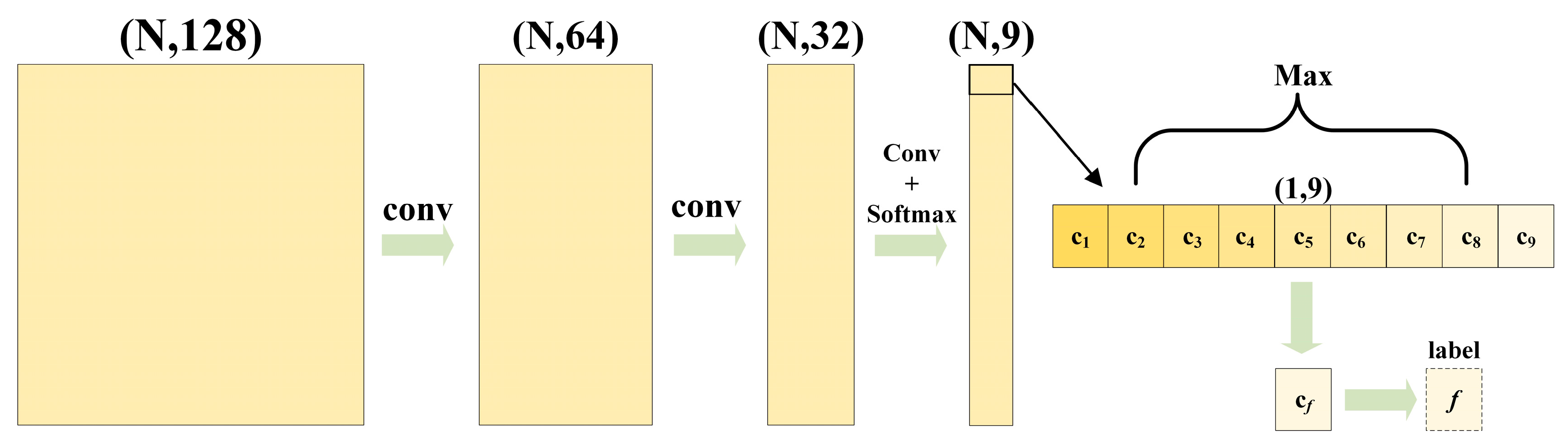
The original point cloud features are supplemented through upsampling, which can realize semantic segmentation of point clouds. It can be seen from Figure 8 that N × 9 tensor was acquired through multi-layer convolution of significant features gained through above feature propagation. Later, predicted scores of each point were calculated from the Softmax function, and the index corresponding to the maximum score was used as the prediction result. For the training set, the prediction results and real labels were implanted into cross-entropy loss function to calculate losses, implement backpropagation and calculate gradient. Later, weights of the model were updated through the optimizer and the model parameters were optimized. In addition, the validation set is necessary to evaluate and monitor the performance of the model during the training process. In this paper, the preprocessed training set was divided into a training subset and a validation subset according to the ratio of 8:2. The hyperparameters were adjusted according to the training and validation effects, and then the adjusted hyperparameters were used to train the original training set. The model was trained from scratch until reaching the optimal solution. The above trained model was tested by using the test set. A nine-dimensional vector of each point was output according to forward propagation. This vector expresses the probability for each point belonging to each of the nine categories . The index f corresponding to the maximum probability was used as the corresponding tag to be distributed to each point and used as the semantic segmentation results of each point in the test set.
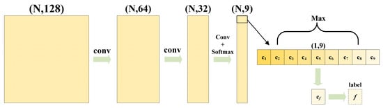
Figure 8.
Semantic labeling.
3. Results
3.1. Brief Introduction to Experimental Data
The experiment used the Germany Vaihingen Town 3D Semantic Labeling Contest dataset provided by International Society for Photogrammetry and Remote Sensing (ISPRS) [47,48]. There are 753,876 and 411,722 points in the training set and test set, where the distribution of the LiDAR point cloud data and the corresponding geo-referenced IR-R-G images are shown in Figure 9a and Figure 9b, respectively. These point cloud data were acquired based on the Leica ALS 50 system at an average altitude of 500 m above ground level. There were four points in each square meter and each laser point contains 3D point coordinates, laser intensity, return number, number of returns and corresponding semantic labels. Geo-referenced images of the entire data area have a ground sampling distance of 8 cm. The training set located in a residential area is mainly composed of buildings, vegetation and impervious surface, supplemented by few other surface features, covering an area of 399 m × 421 m. The test set is centered at Vaihingen City where has diversified surface features in dense distributions with an area of 389 m × 419 m. Unlike the training set, there are large mixed regions of shrubs and trees in addition to common surface features. The Vaihingen dataset is a typical urban surface dataset and the competition official divides surface features in the dataset into nine categories, which are powerline (pow), low vegetation (l_veg), impervious surfaces (i_surf), car, fence/hedge (f_hedge), roof, façade (fac), shrub and tree. Statistics of points in each category are shown in Table 1. Specifically, there are more points in the low vegetation, impervious surfaces, roofs, shrubs and trees categories, which are the keys of semantic segmentation. The rest surface categories with small quantities, such as powerline, car, fence/hedge, and façade, are challenges of semantic segmentation. The Vaihingen dataset contains complex and irregular surface features with rich geo-graphic environments, urban environments and buildings, which can fully validate the performance of the proposed model in urban scenes.
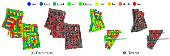
Figure 9.
Vaihingen dataset.

Table 1.
Point quantity of different categories in Vaihingen dataset.
3.2. Network Parameters
The proposed method was implemented using the PyTorch framework based on NVIDIA GeForce GTX1070 8G GPU. Model design parameters of the proposed method are mainly based on PointNet++ [18]. In the preprocessing of original data, the sampling block size was set 15 × 15 and 5 was chosen as the sliding step length. In each block, a total of 1024 points were chosen for sampling. There were 256, 64, and 16 centroids for group sampling in each feature extraction layer. The two radii in multi-scale BQ were [0.05, 0.1], [0.1, 0.2], and [0.2, 0.4], respectively. There were 8 heads in MAM. In model training, the batch size was set 16 and 200 epoch was trained. The Adam [49] optimizer with a learning rate of 0.001 and an attenuation step length of 10 was used. The learning rate showed exponential attenuation with the increase of iteration times.
3.3. Experimental Results and Analysis
3.3.1. Accuracy Evaluation Metrics
The ability of the proposed SMAnet was evaluated quantitatively by using common metrics for semantic segmentation of point clouds, including overall accuracy (OA), time complexity, precision, recall, and comprehensive evaluation metric (F1-score). Time complexity is the model inference time for the test set. Precision is the proportion of all points predicted by the classifier to be in the category that are accurately classified. Recall is the proportion of accurately classified points in total points of the category. F1-score is an index to measure model accuracy and it is defined as the harmonic average of precision and recall, and it is ranged between 0 and 1. OA is the proportion of accurately classified samples in total samples. The calculation formulas are shown in Equation (10).
where ZTP is the number of true positives, ZTN is the number of true negatives, ZFP is the number of false positives, and ZFN is the number of false negatives.
3.3.2. Overall Performance
The standard data for semantic segmentation of point clouds in Vaihingen is provided by ISPRS 3D Semantic Labeling Contest. With references to ISPRS 3D competition, the quantitative performance metrics, including OA, precision, recall, F1-scores and Time, were chosen to evaluate segmentation accuracy of the SMAnet model. The classification results of SMAnet and amplification results of three blocks are shown in Figure 10. The confusion matrix statistics of classification results are presented in Table 2, with the OA is 85.7% and Time is 47 s. According to analysis of Figure 10 and Table 2, SMAnet can achieve good semantic segmentation for most surface objects.
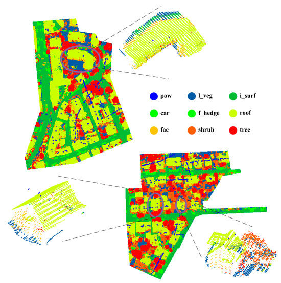
Figure 10.
Experimental results of SMAnet (amplification of three local areas are shown in the circle).
Table 2.
Confusion matrix of SMAnet classification results (OA = 85.7%, Time = 47 s).
The confusion matrix was analyzed based on the probability (recall) of correctly classified points in each category. The SMAnet model achieves the best performances in powerline, impervious surfaces and roof, with a segmentation accuracy of 90.8%, 91.1%, and 93.1%, respectively. The model can distinguish point clouds in the mixing region with similar features very well, such as powerline and roof, roof and façade, impervious surfaces and low vegetation. However, it has moderate segmentation performances to fence/hedge, façade and shrub, showing a segmentation accuracy of 51.1%, 59.6% and 53.8%, respectively. The fence/hedge is often difficult to distinguish from other categories. Specifically, 21.5% fence/hedge points are wrongly classified as shrubs, and 16.1% fence/hedge points are wrongly classified as trees. This is due to the fact that shrubs and trees have similar performances with fence/hedge in term of spatial structure, geometric features and spectral reflectance. Since façade and roof are both components of buildings, façade is easy to be mixed with adjacent shrubs and trees. Hence, façade points are mainly wrongly classified into roof, shrub and trees by 10.9%, 10.8%, and 10.2%, respectively. Shrub is mainly wrongly classified as low vegetation and trees by 12.4% and 20.8%, respectively. This is mainly caused by elevation similarity between shrub and low vegetation, and shrub has similar structural and topological relations with tree, thus resulting in the low classification precision of shrub. Besides, shrub and tree are major cause of confused semantic segmentation of most point clouds, and most surface features are wrongly classified as shrub or tree. This is due to the fact that shrub and tree are similar with most surface features and there are mixed point clouds at boundaries. Moreover, shrub and tree have similar geometric features and they are difficult to be distinguished effectively. Although this can be improved by establishing connections among different types of points, semantic segmentation of point clouds of highly similar surface features such as fence/hedge, shrub and tree is still a great challenge.
4. Discussion
4.1. Comparative Experiments
To further verify performances of the SMAnet model, it was compared with 8 competition results provided by ISPRS 3D Semantic Labeling Contest. The IIS_7 [50] makes supervoxel segmentation of LiDAR data such as shape, color and strength, and extracts spectral and geometric features of hypervoxels by using them as the processing units. Each point is marked by KNN classifier. The UM [51] method input several features of point-like attribute information, texture information, and geometric attributes into the one-to-one classifier for semantic segmentation. The HM_1 [52] is determined by geometric features of point neighborhood and performs semantic analysis of point clouds by using RF classifier [8]. The WhuY3 [53] method transforms 3D spatial features of point clouds into 2D image features and then classifies point clouds successfully by the high-level expression of CNN extracted features. The LUH [54] designs a two-layer CRF framework and increases classification precision by iteration and context propagation of the framework. The BIJ_W [55] method proposes a pooling based on distance minimum spanning tree to process point features and increase semantic segmentation precision of point clouds. Based on the 3D coordinates and corresponding spectral information, The RIT_1 [56] method designs an end-to-end 1D fully convolutional network. The NANJ2 [57] method learns based on the deep-layer features of image context based on multi-scale CNN.
Result statistics of the proposed SMAnet model and above eight methods are listed in Table 3, mainly including F1-scores of different types of surface features, OA, average F1-score (A.F1), and Time. It can be understood from the comparative analysis that the SMAnet model shows the best general performances. The OA and average F1-scores of the SMAnet model reach 85.7% and 75.1%, which are 0.5% and 5.8% higher than those of NANJ2 method provided by the Contest. The SMAnet improves the segmentation effect of fence/hedge and façade the mostly. Its F1-scores are 11.8% and 10.1% higher compared to those of NANJ2 and LUH methods. In particular, the maximum improvement is achieved when there are limited training samples of fence/hedge and façade. Besides, SMAnet also achieves good effect in classification of powerline, car, façade and tree. NANJ2 achieves the best segmentation performances for low vegetation and shrub, and F1-scores are both 4.9% higher than that of SMAnet. This is due to the fact that the NANJ2 can learn deep-layer features better by using the multi-scale CNN. With respect to impervious surfaces, F1-scores of HM_1 and RIT_1 methods are both 0.1% higher than that of SMAnet. This is due to the fact that the HM_1 method can classify some surface points very well by using artificial features. RIT_1 extracts spectral features by using fully convolutional network (FCN), which is beneficial for extraction of Impervious surfaces. For roof, SMAnet and LUH show similar F1-scores and the F1-scores of LUH is 0.1% higher. This is due to the fact that LUH which uses voxel segmentation technique is more beneficial for semantic segmentation of point clouds of roof. Due to the model complexity, the model inference time in this paper does not reach the highest degree of the competition results. However, the SMAnet has some advantages in terms of segmentation accuracy and computational efficiency.
Table 3.
Experimental results (%) of different algorithms for ISPRS 3D Semantic Labeling Contest.
Except for comparison with the above methods, this study further compared the proposed SMAnet with PointNet [17], PointNet++ [18], PointSIFT [19], DGCNN [20], RandLANet [27], A_PointNet++ [28], GADHNet [31] and PCT [33] which have been proposed in recent years. Particularly, the DGCNN is a graph-based convolutional semantic segmentation model, the GADHNet and PCT are semantic segmentation models based on attention mechanisms. These eight models can process the original point cloud data directly, without need of rasterization of point clouds. Hence, they provide great contributions to semantic segmentation of point clouds. The results of different models are listed in Table 4. Results of different models all come from test results of open-source codes or publicly available results from papers using the same data. According to our observations, SMAnet achieves the optimal results in semantic segmentation of most surface features. Its average F1-scores and OA are 2.5% and 1.1% higher than those of the optimal reference baseline PointSIFT provided by Table 4. Moreover, the F1-scores of each surface features of the SMAnet are on average 0.4% higher than the optimal F1-scores of different surface features. For powerlines, impervious surfaces and cars, the F1 scores of A_PointNet++ are 3.5%, 0.3% and 0.3% higher than the models proposed in this paper, respectively. This is due to the fact that the former is able to distinguish surface feature points with similar elevations well by using adaptive elevation interpolation. Since the GADHNet model uses the elevation attention module to establish the point cloud elevation feature connection, it can distinguish between the uniformly distributed roof points. PointSIFT offsets insufficient neighborhood information through resampling in eight neighborhoods, thus increasing the segmentation precision of shrub by 0.1% compared to that of SMAnet. In addition, compared to other complex models, the model in this paper has low computational complexity, can inference the data quickly, and has strong practicality.
Table 4.
Semantic segmentation results (%) of different models.
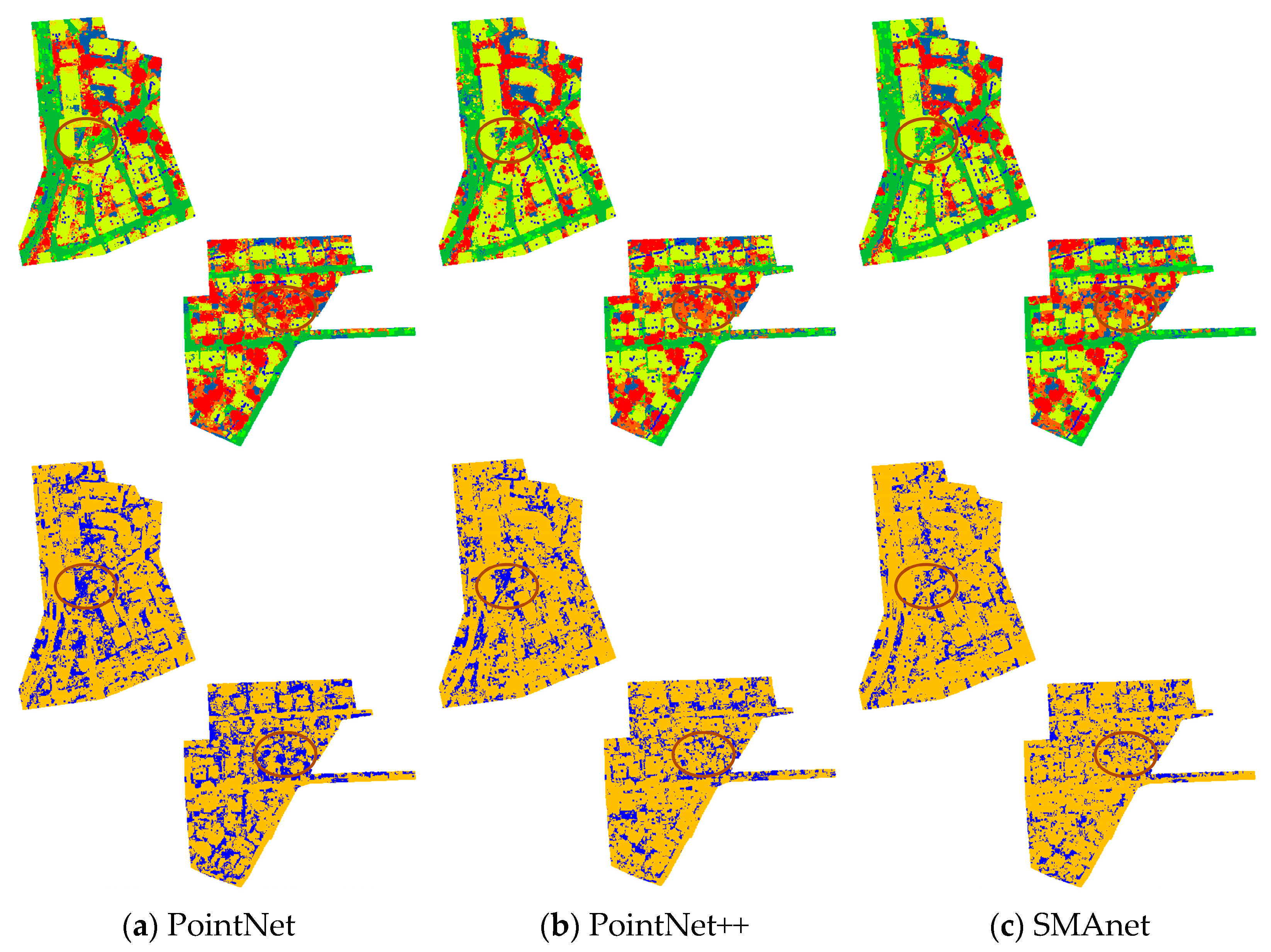
For visual interpretation of experimental results, two representative models of PointNet and PointNet++ were chosen. Results of PointNet and PointNet++ as well as the proposed SMAnet were displayed for qualitative analysis. PointNet is the pioneer of semantic segmentation of point clouds and PointNet++ is the improved version of PointNet. Based on PointNet++, this study further proposed the SMAnet model. The semantic segmentation results (upper rows) and positive-negative chart (lower rows) of three models under the test set are shown in Figure 11. By comparing the results in the ellipses in the figure, experimental results of PointNet and PointNet++ have obvious wrong classifications. In particular, they have low classification precisions in the mixing distribution regions of point clouds, such as of buildings and trees, or shrubs and trees, as shown in Figure 11a,b. The SMAnet model can inhibit such wrong classification effectively and its classification precision is improved significantly compared to those of the PointNet and PointNet++ models.
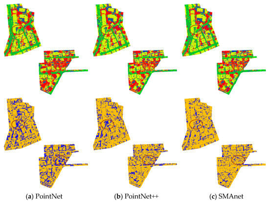
Figure 11.
Semantic segmentation and positive-negative charts of PointNet, PointNet++ and SMAnet models, In the positive-negative chart, yellow shows points that were correctly classified and blue shows points that were incorrectly classified.
4.2. Ablation Experiments
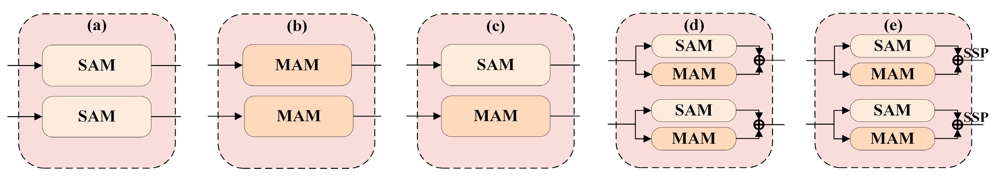
To better understand influences of various strategies on precision of the SMAnet model, an ablation experiment was carried out in this section by adding and subtracting modules flexibly to compare abilities of different strategies. A total of six strategies were designed based on the SAM (S) module, MAM (M) module, fusion attention mechanism (SM) and softmax-based stochastic pooling (SSP). Different strategic designs are shown in Figure 12. SMAnet (BASE) has no attention module and extracts features by multi-scale sampling, and extracts global information through MP. SMAnet (S) and SMAnet (M) means to apply SAM or MAM modules based on SMAnet (BASE). SMAnet (S+M) uses different attention modules based on two scales of paths in multi-scale feature extraction. One path uses SAM module and the other path uses MAM module. SMAnet (SM) combines fusion attention mechanism and MP. SMAnet (SM+SSP) is the proposed model in this study. This mode uses fusion attention mechanism and SSP aggregation function.
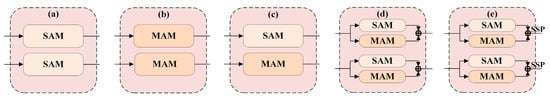
Figure 12.
Schematic diagram of different strategies, (a) SMAnet (S), (b) SMAnet (M), (c) SMAnet (S+M), (d) SMAnet (SM), and (e) SMAnet (SM+SSP).
Statistics of experimental results of different strategies are shown in Table 5. The average F1-scores and OA of other five strategies are higher than those of SMAnet (BASE), indicating that S, M, SM modules and SSP aggregation function are all conducive to improve performances of models. SMAnet (M) has higher F1-scores than SMAnet (S) for most surface features. The F1-scores of SMAnet (M) are 9.0% and 9.4% higher in term of fence/hedge and shrub. This is due to the fact that the M module gives full considerations to deep connections of all aspects of discrete points. This is beneficial for distinguishing point clouds (e.g., fence/hedge and shrub) which have different scales and different shapes. For point clouds (e.g., powerline, car and roof) which are easy to be confused with other categories, SMAnet (S) shows better performances. Additionally, the SMAnet (SM) strategy which uses two attention modules simultaneously is superior to the model using single attention module or the SMAnet (S+M) model, showing the reasonability of the fusion attention module. In particular, F1-scores of SMAnet (SM) on most surface features are higher than those of SMAnet (S+M). This is due to the fact that SMAnet (S+M) considers only global information or subspace information in high-dimensional features, while SMAnet (SM) considers close connections among point clouds from perspectives of global information and subspace information. The average F1-scores of SMAnet (SM+SSP) are 1.3% higher than those of SMAnet (SM). This is due to the fact that SSP aggregation function can expand the receptive field of network very well, increases utilization of global information, and assures segmentation precision of the model. Although the different modules increase the computational complexity of the model, it is worth it for the increase in segmentation accuracy. To sum up, the SMAnet (SM+SSP) model has good performances in most surface features and it is applicable to semantic segmentation of point clouds well.
Table 5.
Ablation experimental results (%).
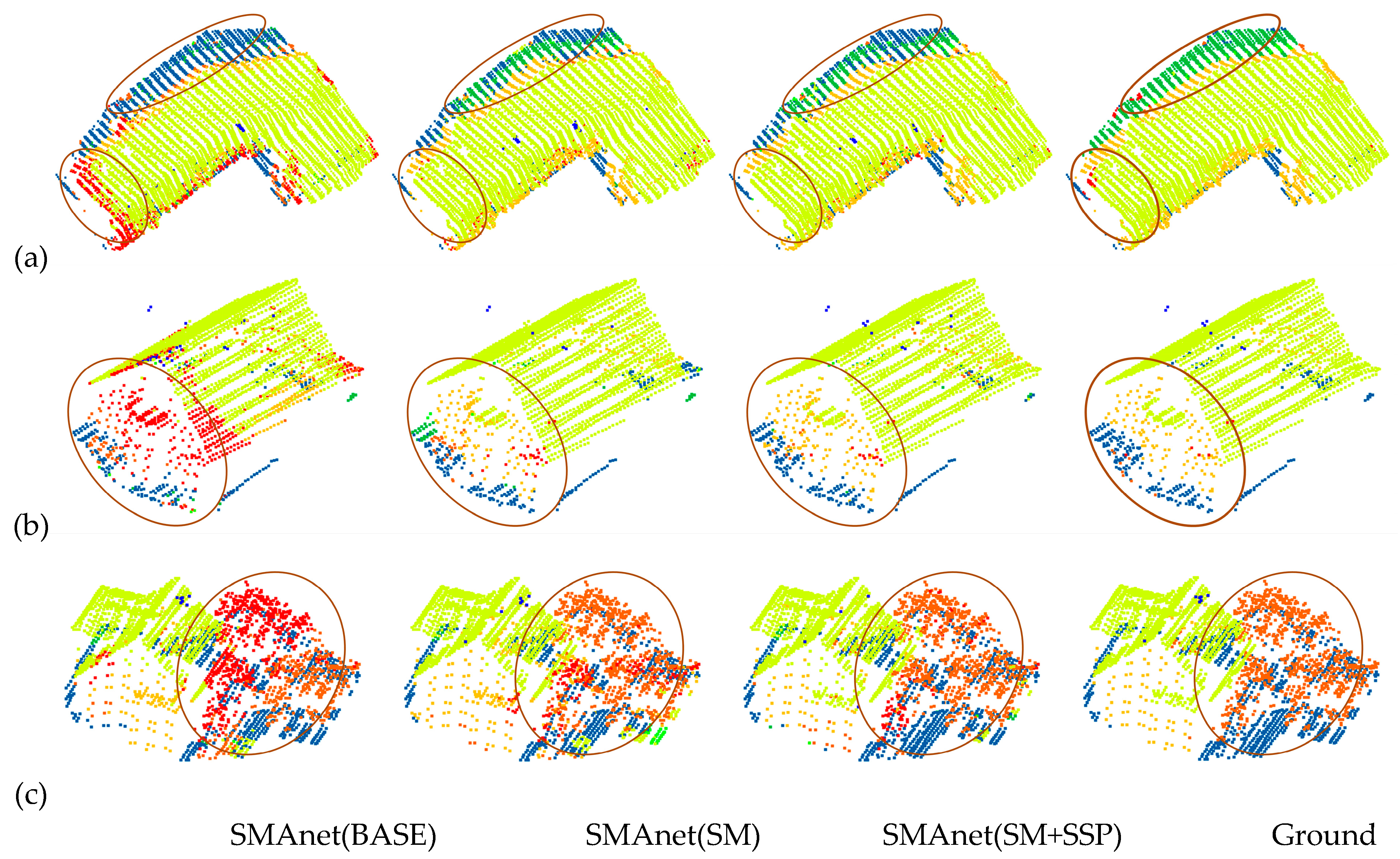
For more intuitive observation and analysis of experimental results of different strategies, three representative areas in the test set were chosen and displayed as Figure 13a–c. They are from typical regions in the test set, as shown in oval regions in Figure 10. All three areas are in the mixing region. Semantic segmentation results of SMAnet (BASE), SMAnet (SM) and SMAnet (SM+SSP) in three areas are shown in the first three columns in Figure 13. The fourth column is the ground truth provided by ISPRS 3D official website.

Figure 13.
Classification results of SMAnet (BASE), SMAnet (SM), SMAnet (SM+SSP), and Ground Truth of test set (from left to right). Area (a) is the mixing region of houses with surrounding affiliated Impervious surfaces and low vegetation. Area (b) covers houses and low vegetation. Area (c) is the mixing region composed of independent houses, low vegetation and surrounding shrub and trees.
Qualitative analyses of the ablation experiments were carried out according to the elliptical circles in Figure 13. With respect to classification results in Area (a), SMAnet (BASE) achieves relatively poor classification results, while the other two strategies based on the SM module of the fusion attention mechanism can distinguish point clouds of mixed surface features very well (for example, point clouds of surface features with similar structures, such as impervious surface and low vegetation, as well as façade and tree). This is due to the fact that SM can establish the global dependence relations among features effectively. In Area (b), SMAnet (BASE) classifies most roof and façade points wrongly as tree points. SMAnet (SM+SSP) and SMAnet (SM) both can distinguish the mixed point clouds which are highly similar very well. In treatment of details (the finer points of classification), the precision of SMAnet (SM) declines since it uses MP aggregation function that may loose some important features. SMAnet (SM+SSP) can process details of point clouds in mixing regions well, since it uses SSP aggregation function that can increase information utilization very well and capture important features, thus increasing semantic segmentation precision. For the shrub point clouds of different scales in Area (c), SMAnet (BASE) is easy to classify shrub wrongly as tree, thus decreasing classification precision. SMAnet (SM+SSP) can distinguish shrubs which have complicated structures and different scales very well. In a word, SMAnet (SM+SSP) can distinguish point clouds of mixed surface features very well and shows good segmentation performances to surface features with irregular structures.
4.3. Experiments with the Number of Heads of MAM
Additionally, the following experiment was designed to verify influences of number of attention heads in MAM on capture of local feature subspace information. Based on the SMAnet model, this experiment kept the SAM module and implemented training and testing by using MAM with 2, 4, 8, and 16 heads. The results are shown in Table 6. It can be found when there are 8 heads, the SMAnet model achieved the highest average F1-scores and OA. If there are few heads, it is easy to capture insufficient local feature subspace information. Hence, the precision increases with the increase of heads. However, excessive subspaces may affect precision [58] and inference time, bringing information redundancy and making it difficult to capture accurate information.
Table 6.
Effects of head number in MAM on experimental results (%).
4.4. Experiments on Grid Sampling Parameters
To verify the effect of data preprocessing on the proposed model, different grid sampling strategies are selected for experiments. The experimental results are shown in Table 7, where S_Points represents the number of points sampled in the block, and P_Time represents the time of data preprocessing. It is observed that the sampling strategy with 15 × 15 block size can be well applied to the proposed SMAnet model. Large block size will lose a lot of point cloud information, leading to poor classification accuracy. The mall block size contains less information in the local area, which is not conducive to the SMAnet model establishing the feature connection between different points, and generates extra computation time.
Table 7.
Experimental results (%) of different grid sampling strategies.
4.5. Experiments with the GML(B) Dataset
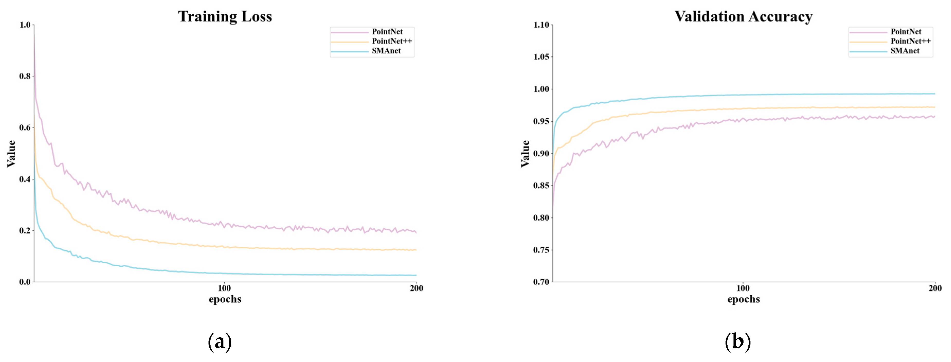
To verify the generalization ability of the SMAnet model, we performed generalization experiments on the GML(B) [59] dataset. The GML(B) dataset is acquired by an airborne Leica ALTM 2050 system, and each point only contains spatial coordinate data. It belongs to part B of the GML dataset. GML(B) dataset mainly contains four surface features: ground, buildings, high vegetation (h_ve) and low vegetation (l_ve). The experiments were conducted using the same strategy and hyperparameters as on the Vaihingen dataset. The experimental results are shown in Table 8. From Table 8, it can be seen that SMAnet has good scores in terms of inference time and classification accuracy. The proposed model can achieve better classification results for buildings, high vegetation and low vegetation points. In addition, the training loss curve and the validation accuracy curve of SMAnet are shown in Figure 14. It can be seen that the proposed model performs well, achieves a low loss, and obtains a high accuracy.
Table 8.
Experimental results (%) of different models on GML(B) dataset.
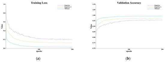
Figure 14.
(a) Training loss curves and (b) validation accuracy curves for PointNet, PointNet++ and SMAnet.
5. Conclusions
In this study, a SMAnet framework is proposed based on PointNet++. Compared with PointNet++, the SMAnet model has the following three characteristics: (1) The SMAnet model strengthens feature associations of points and supplements semantic information of each point by integrating fusion attention mechanism into the process of feature extraction. The fusion attention mechanism is composed of SAM and MAM. The SAM establishes associations through global features of points, enhances important feature channels, and overcomes difficulties in classifying mixed point clouds at boundaries of different semantic surface features. The MAM establishes internal associations of the containing features in feature subspaces of different points to explore the deep associations of point clouds. It extracts semantic associations among points more comprehensively and can classify point clouds of the same surface feature which has different scale and shapes very well. (2) SMAnet extracts multi-scale features by using the light feature learning framework and supplements local information. It considers both computational efficiency and segmentation precision. (3) The global information is extracted based on SSP. It extracts information in feature spaces selectively, expands receptive field of the network, and increases precision of semantic segmentation. The proposed model performs well on both GML(B)dataset and Vaihingen dataset.
Nevertheless, the SMAnet has the following limitations: (I) Block sampling of dataset may lose some key points. The original point cloud information will be supplemented by improved grid sampling algorithms in subsequent studies. (II) There are still poor classification precision on some surface features, such as fence/hedge and shrub. Fence/hedge and shrub are adjacent to other categories and they are difficult to distinguish effectively. It is suggested that one supplies additional relevant information such as local neighborhood geometry information in feature extraction. (III) The SSP may loose some important features since the extraction of features based on probabilities is random, which requires further constraints. In the future, the proposed model will be improved to accommodate more point cloud data, such as noisy and incomplete point clouds. Consideration is given to encoding local region point clouds through geometric and relative position information, thus complementing the neighborhood information. The attention mechanism can also be embedded into the pooling algorithm so that the network can focus on global feature extraction. In addition, reducing the computation time by designing a more lightweight framework is also a strategy to improve the performance of the model.
Author Contributions
H.L. designed the workflow and conducted the experiments, and was responsible for the main structure and writing of the paper; H.L. and J.W. discussed the results described in the paper and analyzed them; J.W., Z.X. and X.X. provided comments and suggestions on the writing of the paper. All authors have read and agreed to the published version of the manuscript.
Funding
This research was funded by the National Natural Science Foundation of China with Project No. 41871379, the Liaoning Revitalization Talents Program with Project No. XLYC2007026, the Fundamental Applied Research Foundation of Liaoning Province with Project No. 2022JH2/101300273 and No. 2022JH2/101300257.
Data Availability Statement
We sincerely thank the 3D Semantic Labeling Vaihingen dataset provided by International Society for Photogrammetry and Remote Sensing (ISPRS) https://www.isprs.org/education/benchmarks/UrbanSemLab/default.aspx (accessed on 23 November 2022). The GML (B) dataset URLs are available from https://github.com/bwf124565/data (accessed on 11 October 2023). The data and code presented in this study are available on request from the corresponding author.
Conflicts of Interest
The authors declare no conflict of interest.
References
- Guo, Y.; Wang, H.; Hu, Q.; Liu, H.; Liu, L.; Bennamoun, M. Deep Learning for 3D Point Clouds: A Survey. IEEE Trans. Pattern Anal. Mach. Intell. 2021, 43, 4338–4364. [Google Scholar] [CrossRef]
- Jing, Z.; Guan, H.; Zang, Y.; Ni, H.; Li, D.; Yu, Y. Survey of Point Cloud Semantic Segmentation Based on Deep Learning. J. Front. Comput. Sci. Technol. 2021, 15, 1–26. [Google Scholar] [CrossRef]
- Yang, B.; Haala, N.; Dong, Z. Progress and perspectives of point cloud intelligence. Geo-Spat. Inf. Sci. 2023, 26, 189–205. [Google Scholar] [CrossRef]
- Wahabzada, M.; Paulus, S.; Kersting, K.; Mahlein, A.K. Automated interpretation of 3D laserscanned point clouds for plant organ segmentation. BMC Bioinform. 2015, 16, 248. [Google Scholar] [CrossRef] [PubMed]
- Grilli, E.; Menna, F.; Remondino, F. A review of point clouds segmentation and classification algorithms. Int. Arch. Photogramm. Remote Sens. Spat. Inf. Sci. 2017, 42, 339–344. [Google Scholar] [CrossRef]
- Zhang, J.; Lin, X.; Ning, X. SVM-Based Classification of Segmented Airborne LiDAR Point Clouds in Urban Areas. Remote Sens. 2013, 5, 3749–3775. [Google Scholar] [CrossRef]
- Sun, J.; Lai, Z. Airborne LiDAR Feature Selection for Urban Classification Using Random Forests. Geomat. Inf. Sci. Wuhan Univ. 2014, 39, 1310–1313. [Google Scholar] [CrossRef]
- Zhuang, Y.; Liu, Y.; He, G.; Wang, W. Contextual classification of 3D laser points with conditional random fields in urban environments. In Proceedings of the 2015 IEEE/RSJ International Conference on Intelligent Robots and Systems (IROS), Hamburg, Germany, 28 September–2 October 2015; pp. 3908–3913. [Google Scholar] [CrossRef]
- Lu, Y.; Rasmussen, C. Simplified markov random fields for efficient semantic labeling of 3D point clouds. In Proceedings of the 2012 IEEE/RSJ International Conference on Intelligent Robots and Systems, Vilamoura-Algarve, Portugal, 7–12 October 2012; pp. 2690–2697. [Google Scholar] [CrossRef]
- LeCun, Y.; Bengio, Y.; Hinton, G. Deep learning. Nature 2015, 521, 436–444. [Google Scholar] [CrossRef] [PubMed]
- Su, H.; Maji, S.; Kalogerakis, E.; Learned-Miller, E. Multi-View Convolutional Neural Networks for 3D Shape Recognition. In Proceedings of the 2015 IEEE international conference on computer vision (ICCV), Santiago, Chile, 7–13 December 2015; pp. 945–953. [Google Scholar] [CrossRef]
- Boulch, A.; Guerry, J.; Saux, B.L.; Audebert, N. SnapNet:3D point cloud semantic labeling with 2D deep segmentation networks. Comput. Graph. 2018, 71, 189–198. [Google Scholar] [CrossRef]
- Wu, B.; Wan, A.; Yue, X.; Keutzer, K. SqueezeSeg: Convolutional Neural Nets with Recurrent CRF for Real-Time Road-Object Segmentation from 3D LiDAR Point Cloud. In Proceedings of the 2018 IEEE International Conference on Robotics and Automation (ICRA), Brisbane, QLD, Australia, 21–25 May 2018; pp. 1887–1893. [Google Scholar] [CrossRef]
- Maturana, D.; Scherer, S. VoxNet: A 3D Convolutional Neural Network for real-time object recognition. In Proceedings of the 2015 IEEE/RSJ International Conference on Intelligent Robots and Systems (IROS), Hamburg, Germany, 28 September–2 October 2015; pp. 922–928. [Google Scholar] [CrossRef]
- Tchapmi, L.; Choy, C.; Armeni, I.; Gwak, J.; Savarese, S. SEGCloud: Semantic Segmentation of 3D Point Clouds. In Proceedings of the 2017 International Conference on 3D Vision (3DV), Qingdao, China, 10–12 October 2017; pp. 537–547. [Google Scholar] [CrossRef]
- Wang, L.; Huang, Y.; Shan, J.; He, L. MSNet: Multi-Scale Convolutional Network for Point Cloud Classification. Remote Sens. 2018, 10, 612. [Google Scholar] [CrossRef]
- Qi, C.R.; Su, H.; Mo, K.; Guibas, L.J. Pointnet: Deep learning on point sets for 3D classification and segmentation. In Proceedings of the 2017 IEEE Conference on Computer Vision and Pattern Recognition (CVPR 2017), Honolulu, HI, USA, 21–26 July 2017; pp. 77–85. [Google Scholar] [CrossRef]
- Qi, C.R.; Yi, L.; Su, H.; Guibas, L.J. Pointnet++: Deep hierarchical feature learning on point sets in a metric space. In Proceedings of the Neural Information Processing Systems (NIPS 2017), Long Beach, CA, USA, 4–7 December 2017; pp. 5105–5114. [Google Scholar]
- Jiang, M.; Wu, Y.; Zhao, T.; Zhao, Z.; Lu, C. PointSIFT: A SIFT-like Network Module for 3D Point Cloud Semantic Segmentation. arXiv 2018, arXiv:1807.00652. [Google Scholar]
- Wang, Y.; Sun, Y.; Liu, Z.; Sarma, S.E.; Bronstein, M.M.; Solomon, J.M. Dynamic graph CNN for learning on point clouds. ACM Trans. Graph. 2018, 38, 1–12. [Google Scholar] [CrossRef]
- Zhao, H.; Jiang, L.; Fu, C.W.; Jia, J. PointWeb: Enhancing Local Neighborhood Features for Point Cloud Processing. In Proceedings of the 2019 IEEE/CVF Conference on Computer Vision and Pattern Recognition (CVPR), Long Beach, CA, USA, 15–20 June 2019; pp. 5560–5568. [Google Scholar] [CrossRef]
- Xie, S.; Liu, S.; Chen, Z.; Tu, Z. Attentional ShapeContextNet for Point Cloud Recognition. In Proceedings of the 2018 IEEE/CVF Conference on Computer Vision and Pattern Recognition, Salt Lake City, UT, USA, 18–23 June 2018; pp. 4606–4615. [Google Scholar] [CrossRef]
- Landrieu, L.; Simonovsky, M. Large-Scale Point Cloud Semantic Segmentation with Superpoint Graphs. In Proceedings of the 2018 IEEE/CVF Conference on Computer Vision and Pattern Recognition, Salt Lake City, UT, USA, 18–23 June 2018; pp. 4558–4567. [Google Scholar] [CrossRef]
- Li, Y.; Bu, R.; Sun, M.; Wu, W.; Di, X.; Chen, B. PointCNN: Convolution On χ-Transformed Points. In Proceedings of the Annual Conference on Neural Information Processing Systems (NeurIPS 2018), Montréal, QC, Canada, 3–8 December 2018; pp. 828–838. [Google Scholar]
- Qian, G.; Li, Y.; Peng, H.; Mai, J.; Hammoud, H.; Elhoseiny, M.; Ghanem, B. Pointnext: Revisiting pointnet++ with improved training and scaling strategies. In Proceedings of the Advances in Neural Information Processing Systems (NeurIPS 2022), New Orleans, LA, USA, 28 November–9 December 2022. [Google Scholar]
- Hua, B.S.; Tran, M.K.; Yeung, S.K. Pointwise Convolutional Neural Networks. In Proceedings of the 2018 IEEE/CVF Conference on Computer Vision and Pattern Recognition, Salt Lake City, UT, USA, 18–23 June 2018; pp. 984–993. [Google Scholar]
- Hu, Q.; Yang, B.; Xie, L.; Rosa, S.; Guo, Y.; Wang, Z.; Trigoni, N.; Markham, A. RandLA-Net: Efficient Semantic Segmentation of Large-Scale Point Clouds. In Proceedings of the 2020 IEEE/CVF Conference on Computer Vision and Pattern Recognition (CVPR), Seattle, WA, USA, 13–19 June 2020; pp. 11105–11114. [Google Scholar] [CrossRef]
- Nong, X.; Bai, W.; Liu, G. Airborne LiDAR point cloud classification using PointNet++ network with full neighborhood features. PLoS ONE 2023, 18, e0280346. [Google Scholar] [CrossRef] [PubMed]
- Vaswani, A.; Shazeer, N.; Parmar, N.; Uszkoreit, J.; Jones, L.; Gomez, A.N.; Kaiser, Ł.; Polosukhin, I. Attention is all you need. In Proceedings of the Neural Information Processing Systems (NIPS 2017), Long Beach, CA, USA, 4–7 December 2017; pp. 5998–6008. [Google Scholar]
- Zeng, J.; Wang, D.; Chen, P. A Survey on Transformers for Point Cloud Processing: An Updated Overview. IEEE Access 2022, 10, 86510–86527. [Google Scholar] [CrossRef]
- Li, W.; Wang, F.D.; Xia, G.S. A geometry-attentional network for ALS point cloud classification. ISPRS J. Photogramm. Remote Sens. 2020, 164, 26–40. [Google Scholar] [CrossRef]
- Zhao, H.; Jiang, L.; Jia, J.; Torr, P.; Koltun, V. Point Transformer. In Proceedings of the 2018 IEEE/CVF International Conference on Computer Vision (ICCV), Montreal, QC, Canada, 10–17 October 2021; pp. 16259–16268. [Google Scholar] [CrossRef]
- Guo, M.H.; Cai, J.X.; Liu, Z.N.; Mu, T.J.; Martin, R.R.; Hu, S.M. PCT: Point cloud transformer. Comput. Vis. Media 2021, 7, 187–199. [Google Scholar] [CrossRef]
- Zhang, Z.; Li, T.; Tang, X.; Lei, X.; Peng, Y. Introducing Improved Transformer to Land Cover Classification Using Multispectral LiDAR Point Clouds. Remote Sens. 2022, 14, 3808. [Google Scholar] [CrossRef]
- Nam, H.; Ha, J.W.; Kim, J. Dual Attention Networks for Multimodal Reasoning and Matching. In Proceedings of the 2017 IEEE Conference on Computer Vision and Pattern Recognition (CVPR), Honolulu, HI, USA, 21–26 July 2017; pp. 299–307. [Google Scholar] [CrossRef]
- Xu, T.; Ding, H. Deep Learning Point Cloud Classification Method Based on Fusion Graph Convolution. Laser Optoelectron. Prog. 2022, 59, 0228005. [Google Scholar] [CrossRef]
- Jain, Y.K.; Bhandare, S.K. Min Max Normalization Based Data Perturbation Method for Privacy Protection. Int. J. Comput. Commun. Technol. 2013, 2, 45–50. [Google Scholar] [CrossRef]
- Eldar, Y.; Lindenbaum, M.; Porat, M.; Zeevi, Y.Y. The farthest point strategy for progressive image sampling. IEEE Trans. Image Process. 1997, 6, 1305–1315. [Google Scholar] [CrossRef]
- Ioffe, S.; Szegedy, C. Batch normalization: Accelerating deep network training by reducing internal covariate shift. In Proceedings of the 32nd International Conference on Machine Learning, Lille, France, 6–11 July 2015; pp. 448–456. [Google Scholar]
- Krizhevsky, A.; Sutskever, I.; Hinton, G.E. ImageNet Classification with Deep Convolutional Neural Networks. In Proceedings of the Advances in Neural Information Processing Systems 25 (NIPS 2012), Lake Tahoe, NV, USA, 3–6 December 2012; pp. 1106–1114. [Google Scholar]
- Bouchard, G. Clustering and Classification Employing Softmax Function Including Efficient Bounds. U.S. Patent 8065246, 22 November 2011. [Google Scholar]
- Li, Y. Research on Website Fingerprint Identification Technology of Tor Network; People’s Public Security University of China: Beijing, China, 2022. [Google Scholar] [CrossRef]
- Murray, N.; Perronnin, F. Generalized max pooling. In Proceedings of the 2014 IEEE Conference on Computer Vision and Pattern Recognition (CVPR), Columbus, OH, USA, 23–28 June 2014; pp. 2473–2480. [Google Scholar] [CrossRef]
- Zeiler, M.D.; Fergus, R. Stochastic Pooling for Regularization of Deep Convolutional Neural Networks. arXiv 2013, arXiv:1301.3557. [Google Scholar]
- Fukunaga, K.; Narendra, P.M. A Branch and Bound Algorithm for Computing k-Nearest Neighbors. IEEE Trans. Comput. 1975, C-24, 750–753. [Google Scholar] [CrossRef]
- Setianto, A.; Triandini, T. Comparison of kriging and inverse distance weighted (IDW) interpolation methods in lineament extraction and analysis. J. Appl. Geol. 2013, 5. [Google Scholar] [CrossRef]
- Cramer, M. The DGPF-test on digital airborne camera evaluation-overview and test design. Photogramm.-Fernerkund.-Geoinf. 2010, 2, 73–82. [Google Scholar] [CrossRef] [PubMed]
- Niemeyer, J.; Rottensteiner, F.; Soergel, U. Contextual classification of lidar data and building object detection in urban areas. ISPRS J. Photogramm. Remote Sens. 2014, 87, 152–165. [Google Scholar] [CrossRef]
- Kingma, D.P.; Ba, J. Adam: A Method for Stochastic Optimization. arXiv 2014, arXiv:1412.6980. [Google Scholar]
- Ramiya, A.M.; Nidamanuri, R.R.; Ramakrishnan, K. A supervoxel-based spectro-spatial approach for 3D urban point cloud labelling. Int. J. Remote Sens. 2016, 37, 4172–4200. [Google Scholar] [CrossRef]
- Horvat, D.; Zalik, B.; Mongus, D. Context-dependent detection of non-linearly distributed points for vegetation classification in airborne LiDAR. ISPRS J. Photogramm. Remote Sens. 2016, 116, 1–14. [Google Scholar] [CrossRef]
- Steinsiek, M.; Polewski, P.; Yao, W.; Krzystek, P. Semantische analyse von ALS-und MLS-daten in urbanen gebieten mittels conditional random fields. In Proceedings of the Wissenschaftlich-Technische Jahrestagung der DGPF, Würzburg, Germany, 7–10 March 2017; pp. 521–531. [Google Scholar]
- Yang, Z.; Jiang, W.; Xu, B.; Zhu, Q.; Jiang, S.; Huang, W. A Convolutional Neural Network-Based 3D Semantic Labeling Method for ALS Point Clouds. Remote Sens. 2017, 9, 936. [Google Scholar] [CrossRef]
- Niemeyer, J.; Rottensteiner, F.; Soergel, U.; Heipke, C. Hierarchical higher order crf for the classification of airborne lidar point clouds in urban areas. Int. Arch. Photogramm. Remote Sens. Spatial Inf. Sci. 2016, 41, 655–662. [Google Scholar] [CrossRef]
- Wang, Z.; Zhang, L.; Zhang, L.; Li, R.; Zheng, Y.; Zhu, Z. A Deep Neural Network with Spatial Pooling (DNNSP) for 3-D Point Cloud Classification. IEEE Trans. Geosci. Remote Sens. 2018, 56, 4597–4604. [Google Scholar] [CrossRef]
- Yousefhussien, M.; Kelbe, D.J.; Ientilucci, E.J.; Salvaggio, C. A multi-scale fully convolutional network for semantic labeling of 3D point clouds. ISPRS J. Photogramm. Remote Sens. 2018, 143, 191–204. [Google Scholar] [CrossRef]
- Zhao, R.; Pang, M.; Wang, J. Classifying airborne LiDAR point clouds via deep features learned by a multi-scale convolutional neural network. Int. J. Geogr. Inf. Sci. 2018, 32, 960–979. [Google Scholar] [CrossRef]
- Michel, P.; Levy, O.; Neubig, G. Are sixteen heads really better than one? In Proceedings of the Advances in Neural Information Processing Systems (NeurIPS 2019), Vancouver, BC, Canada, 8–14 December 2019; pp. 14014–14024. [Google Scholar]
- Shapovalov, R.; Velizhev, A.; Barinova, O. Non-Associative Markov Networks For 3d Point Cloud Classification. Int. Arch. Photogramm. Remote Sens. Spat. Inf. Sci. 2010, 38, 103–108. [Google Scholar]


Disclaimer/Publisher’s Note: The statements, opinions and data contained in all publications are solely those of the individual author(s) and contributor(s) and not of MDPI and/or the editor(s). MDPI and/or the editor(s) disclaim responsibility for any injury to people or property resulting from any ideas, methods, instructions or products referred to in the content. |
© 2023 by the authors. Licensee MDPI, Basel, Switzerland. This article is an open access article distributed under the terms and conditions of the Creative Commons Attribution (CC BY) license (https://creativecommons.org/licenses/by/4.0/).