Abstract
Polarimetric Synthetic Aperture Radar (PolSAR) data is inherently characterized by speckle noise, which significantly deteriorates certain aspects of the quality of the PolSAR data processing, including the polarimetric decomposition and target interpretation. With the rapid increase in PolSAR resolution, SAR images in complex natural and artificial scenes exhibit non-homogeneous characteristics, which creates an urgent demand for high-resolution PolSAR filters. To address these issues, a new adaptive PolSAR filter based on joint similarity measure criterion (JSMC) is proposed in this paper. Firstly, a scale-adaptive filtering window is established in order to preserve the texture structure based on a multi-directional ratio edge detector. Secondly, the JSMC is proposed in order to accurately select homogeneous pixels; it describes pixel similarity based on both space distance and polarimetric distance. Thirdly, the homogeneous pixels are filtered based on statistical averaging. Finally, the airborne and spaceborne real data experiment results validate the effectiveness of our proposed method. Compared with other filters, the filter proposed in this paper provides a better outcome for PolSAR data in speckle suppression, edge texture, and the preservation of polarimetric properties.
1. Introduction
Polarimetric Synthetic Aperture Radar (PolSAR) [1] utilizes electromagnetic waves to transmit and receive different polarization modes, which allows it to be highly sensitive to the structural and electromagnetic scattering characteristics of targets [2]. It is widely used in scenarios such as image classification, target detection, and hidden target monitoring [3,4,5,6]. However, the coherent imaging mechanism of SAR still leads to speckle noise in PolSAR data, complicating the data interpretation by reducing the accuracy of image segmentation and classification. Therefore, speckle suppression is crucial for the reformation of PolSAR data quality.
The earliest PolSAR speckle filter was derived from a single-polarization SAR filter, which employs the multi-look averaging method for speckle suppression [1]. Multi-look processing is simple and effective, but at the cost of resolution degradation and spatial detail loss. Therefore, specialized filters for PolSAR data are being explored. The Polarimetric Whitening Filter (PWF) [7] minimizes speckle noise by combining the elements of an optimal-polarization covariance matrix. To reduce the speckle of the three polarimetric channels (HH, HV and VV), J.S. Lee et al. [8] proposed the Optimal Weighted Filter. This filter smooths the PolSAR data linearly based on the multiplicative noise model and Minimum Mean Square Error (MMSE) criterion. Subsequently, Lee proposed the most classic PolSAR spatial filtering algorithm: the Refined Lee Filter (Re-Lee Filter) [9]. The Re-Lee Filter overcomes the restrictions of previous speckle filters by employing span data to determine the edge direction window and related parameters, while also considering speckle suppression and polarization information preservation. Since then, many scholars have carried out in-depth research on the filter and further improved the estimation accuracy of filtering parameters. G. Vasile [10] proposes an adaptive neighborhood (IDAN) filter that combines the region growing technique with the Re-Lee filter. López-Martínez et al. [11,12] explore the realm of spatially nonstationary and anisotropic texture analysis in SAR images and propose a multiplicative-additive speckle noise model to enhance the characterization of speckle effects, particularly on the off-diagonal elements, which are elements of the covariance matrix. Guo [13] and Wu [14] incorporated three-component and four-component decomposition into a PolSAR Re-Lee Filter. In 2018, Xie [15] extended the boundary window of the Re-Lee Filter, simultaneously incorporating statistical models and polarimetric scattering similarity, leading to notable performance improvements. The rise of the Non-Local Mean (NLM) filter has brought a fresh insight to the field of spatial filtering algorithms. In 2009, the concept of Probabilistic Patch-Based (PPB), which is based on noise distribution properties, was introduced in order to determine similarity [16]. Then, Deledalle extended the NLM filter for denoising PolSAR data [17]. In 2015 and 2016, Wu, et al. [18] and Sharifymoghaddam [19] proposed adjustments to the similarity measurement in the NLM algorithm, making it more appropriate for SAR data. NLM filters make use of a wider range of image structure information to estimate similarity and generally perform better at preserving texture information. Nevertheless, they do not demonstrate exceptional performance in maintaining polarimetric properties. To address this, Shen [20] introduced an adaptive NLM filter with shape-adaptive patch matching (ANLM). However, it tends to have a higher algorithmic complexity and lower computational efficiency, making it less practical in large-scale data preprocessing.
Recent advances in machine learning and neural networks have demonstrated great potential for reducing speckle noise in PolSAR data. In a study by Harold C. Burger et al. [21], data denoising was successfully achieved by applying a multilayer perceptron (MLP) to map data blocks and a large database for training. Further research performed by G. Chierchia [22] utilizes a convolutional neural network (CNN) for SAR data denoising. This network applies a residual learning strategy to remove speckle components from the noise data and has achieved impressive results with both synthetic and real SAR data. G. Adugna [23] proposes a multi-stream complex-valued fully convolutional network (CV-deSpeckNet) that reduces speckle and estimates the PolSAR covariance matrix effectively, demonstrating the feasibility of complex-valued deep learning for PolSAR speckle suppression. These filters train deep neural networks on large PolSAR datasets to identify underlying patterns and structures to denoise the data. Despite their high efficacy, it is important to note that these filters require a substantial amount of labeled data and computational resources.
The analysis and review above show that PolSAR speckle suppression has attracted much attention. Conventional spatial domain filters still play a crucial role in practical data processing applications. However, these techniques still have limitations on how accurately they can identify homogeneous pixels. In terms of window selection, traditional windows such as fixed rectangular windows, edge template windows, and adaptive windows are not able to accurately represent the true nature of the ground objects. In terms of judgment criteria, most of the existing algorithms are based on a simple multiplicative speckle noise model and Gaussian distribution statistics, e.g., the confidence interval in the Sigma filter algorithm [24] and the variation coefficient used by the Re-Lee filter [25]. These factors result in errors in the selection of homogeneous pixels and make it challenging to achieve a balance between speckle suppression, preservation of polarization information, and edge structure. To resolve these issues, this paper proposes an adaptive PolSAR speckle filter based on the joint similarity measure criterion (JSMC). Firstly, the multi-directional ratio edge detector and watershed transform are utilized to efficiently acquire an irregular filtering window. Subsequently, we propose the JSMC, which combines spatial-domain and extreme-domain similarity measures to accurately select homogeneous pixels while preserving data characteristics. Finally, statistical averaging is performed on the homogeneous pixels in order to achieve speckle filtering.
The remainder of this paper is structured as follows: The main principles and methods of PolSAR filtering are analyzed in Section 2. In Section 2.1, the fundamental concepts of PolSAR data and the criteria for filter design are briefly introduced. In Section 2.2, the adaptive PolSAR filter based on JSMC is detailed. Based on the analysis above, the complete flow chart of this method is outlined in Section 2.3. The experimental results obtained from both airborne and spaceborne data are presented in Section 3. The performance of the method is further analyzed and discussed in Section 4. Finally, the paper concludes with a summary of its full content in Section 5.
2. Principle and Method of PolSAR Speckle Filtering
2.1. PolSAR Speckle Filtering
PolSAR obtains the medium complex scattering matrix with quad polarizations between the transmitting and the receiving channels. The scattering matrix in the linear polarization base can be expressed as:
The subindices and are the horizontal and vertical orthogonal polarization, respectively. is the scattering element of horizontal transmitting and horizontal receiving polarization, and the other three elements are defined similarly. Based on the hypothesis of reciprocal backscattering case, . The polarimetric scattering information can be represented vectorially by Pauli basis or Lexicographic basis as [26]:
where, the superscript denotes the matrix transpose.
The span (or total power) of a pixel is an incoherent summation of three polarimetric channels (HH, HV and VV), which can be expressed as:
In order to eliminate the speckle caused by the coherent superposition of scattering unit echoes, SAR data are generally filtered by averaging several adjacent single-look pixels. Similarly, the polarization covariance matrix or coherence matrix , after speckle suppression is obtained from the PolSAR data, can be expressed as:
where, is the number of the pixels chosen from the homogeneous region or the number of the nominal multi-look, represents the spatial average of pixels, the superscript , and denote the conjugate transpose and complex transpose.
The covariance matrix and the coherence matrix can be converted through
where,
PolSAR speckle filtering is mainly shown in the accurate statistics of polarization covariance matrix or coherence matrix . The guiding principles are as follows [4].
- Maintain the polarization property:
Each element of the polarimetric covariance matrix or coherence matrix should be estimated by averaging the surrounding homogeneous pixels in a similar way to multi-look processing.
- Avoid crosstalk between polarization channels:
Each element of the polarization covariance matrix or coherence matrix must be filtered independently in the spatial domain. All elements of the covariance matrix should be filtered with the same weight.
- Preserve the edge texture features and point targets:
The filtering should be adaptive and select a homogeneous area from neighboring pixels.
2.2. PolSAR Speckle Filter Based on Joint Similarity Measurement Criterion
The existing spatial PolSAR speckle filters are all implemented by selecting homogeneous pixels for average value. The difference between various filters is only in the selection window algorithm and the homogeneous pixel judgment standard. Considering the above two aspects, this paper will take two measures to ensure the speckle-filtering consequent: construct the irregular filtering window based on the target shape structure and retain the edge features and structure information to the maximum extent and construct JSMC to achieve the selection of homogeneous pixels.
2.2.1. Adaptive Filtering Window Construction
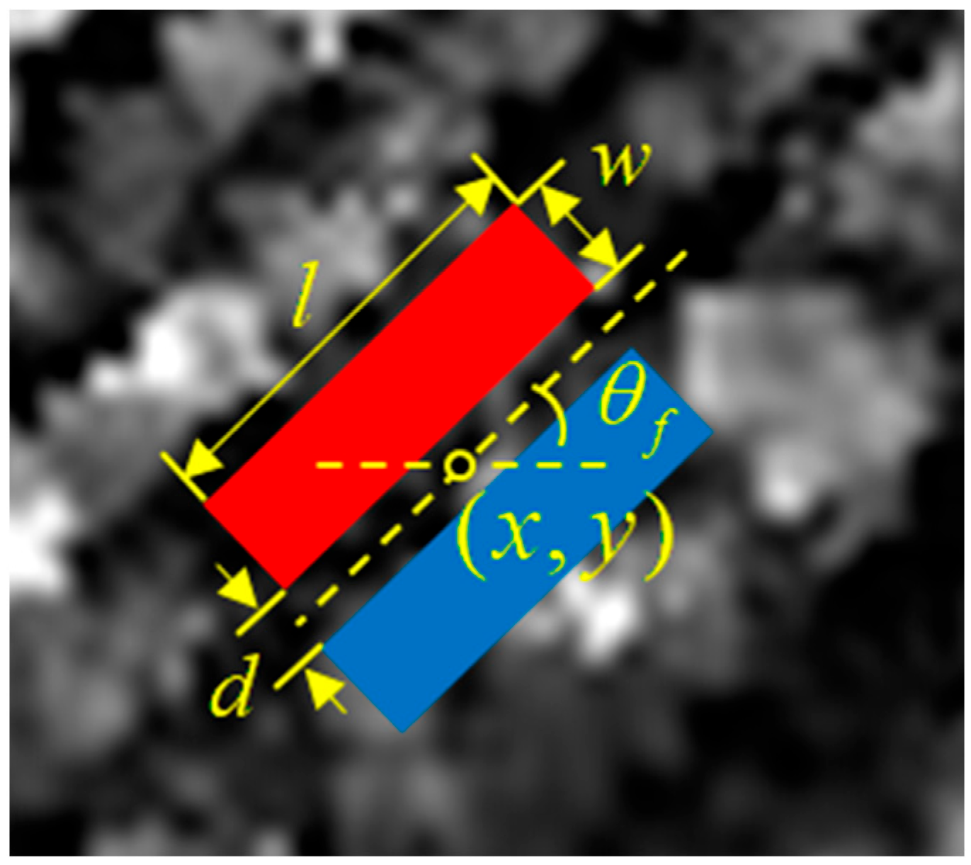
In order to preserve the edge features and structural information, this paper adopts a multi-directional ratio edge detector and watershed transform to construct an adaptive filter window. To prevent the interference of speckle noise with the detection of structural edges, this study employs rotated rectangular windows as edge detectors. An edge detector [27] can be represented by the parameter , and its structure is shown in Figure 1. In Figure 1, is the length of the detector, is the width of the detector, is the width between two rectangles, and is the direction of the detector. For a specific direction , the average value of pixels in the rectangular area on both sides of pixel is and , then the ratio edge strength map (RESM) of the pixel is defined as:
where is uniformly sampled in .

Figure 1.
Configuration of multi-directional ratio edge detector.
To avoid a large number of fragmented windows caused by local minima after watershed transform, this paper utilizes a threshold method to construct the RESM, i.e., in (9), , is the direction number of the edge detector. is the α percentile value of the RESM histogram. The is positively related to the size of the adaptive filtering window, which is the tradeoff between the reduction in speckle and the loss of edge structure. It can be determined according to the demand for filtering details. A larger provides smoother speckle suppression but may blur fine details. If the texture needs to be preserved, a smaller value of should be utilized. Finally, the watershed transform is performed on the threshold RESM to construct the adaptive filtering windows.
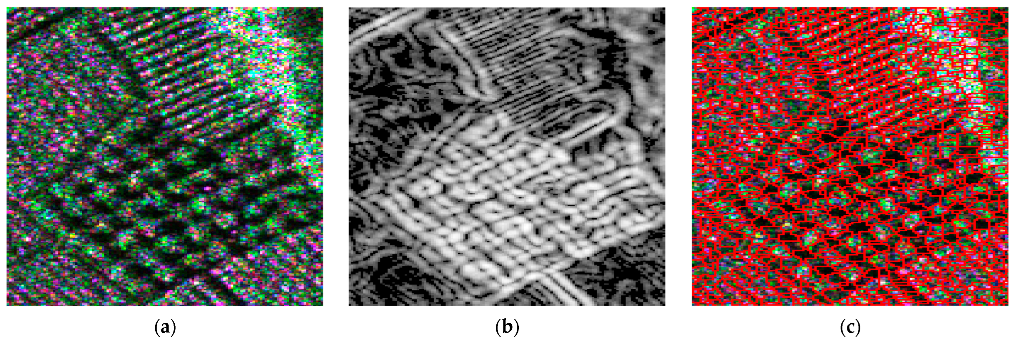
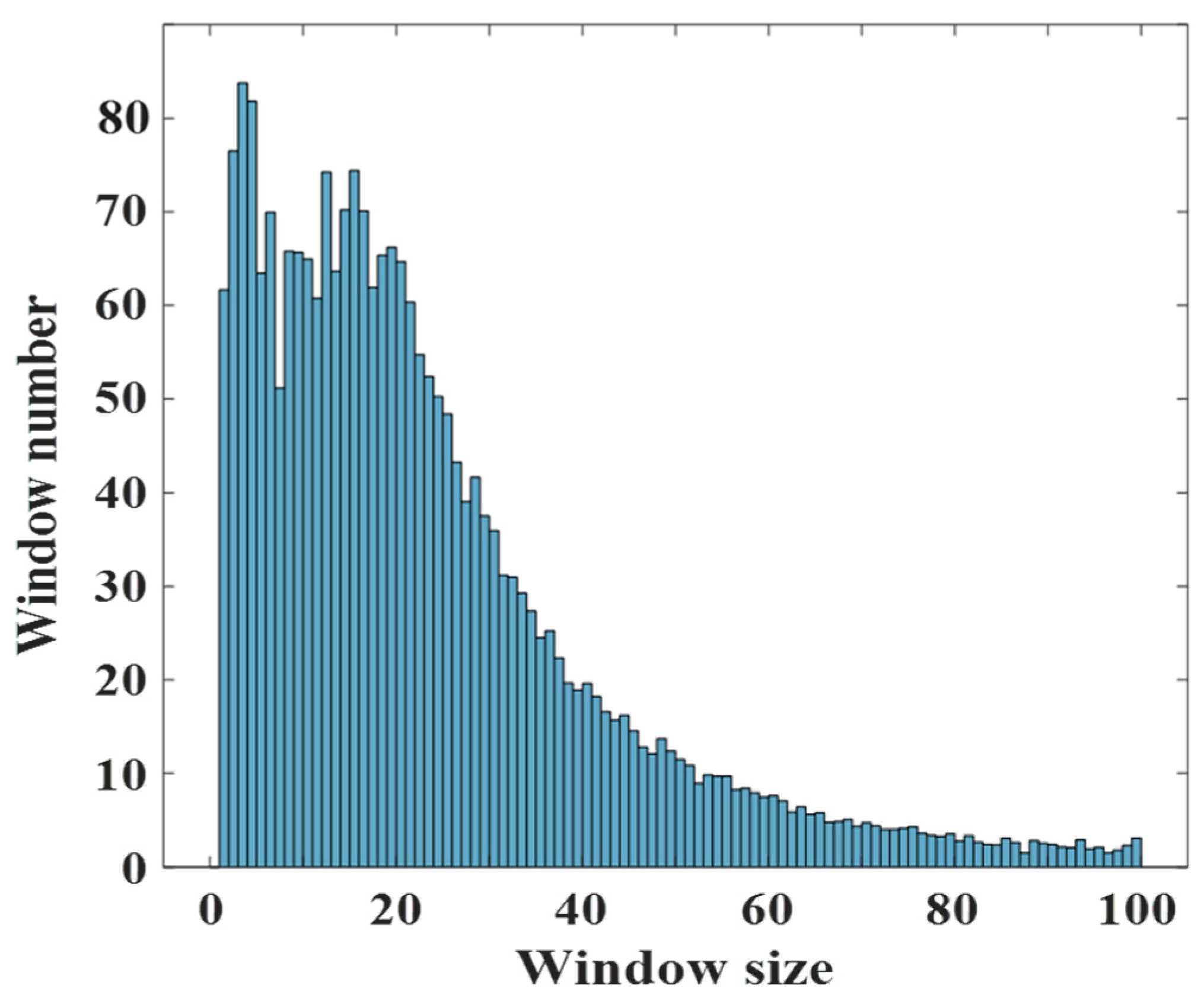
PolSAR span data is the weighted sum of each polarization channel, which can restrain the speckle to a certain extent, and its noise level is lower than that of any polarization channel. Therefore, this paper applies the span data for adaptive filtering window construction. In the following content, the results of adaptive filtering window construction for airborne data are given in Figure 2. The data size is 300 × 300 pixels, and is empirically taken as 20. Figure 2a–c shows a Pauli decomposed diagram of airborne data, threshold RESM, and adaptive filtering windows, respectively. The region primarily consists of grapevines and citrus trees, with grapevines spaced 2–3 pixels apart and citrus trees spaced about 4–5 pixels apart. To ensure that the windows preserve the texture structure, it is certain that a portion of the windows will have smaller sizes, as is shown in Figure 3. However, within the 300 × 300 pixel area of Figure 2, there are a total of 1897 irregular windows, with an average size of 47 pixels, which is roughly equivalent to a 7 × 7 window size. And the window size mainly depends on the geometric structure of the scene, which is consistent with the subjective visual experience.
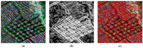
Figure 2.
Adaptive filtering windows based on watershed transform of RESM. (a) Pauli decomposed diagram; (b) its threshold RESM; (c) adaptive filtering windows.

Figure 3.
The size distribution of the adaptive filtering window.
2.2.2. Joint Similarity Measurement Criterion
For SAR data, each pixel is expressed as complex data. For PolSAR data, each pixel is processed with a scattering matrix or covariance matrix, which contains intensity and polarimetric information. Most speckle suppression algorithms refer to the Refined Lee’s filtering idea when extending from SAR to PolSAR filtering, calculate the similarity between pixels to obtain homogeneous pixel areas using PolSAR span data, and then filter each element of the covariance matrix separately. However, it is necessary to retain the polarimetric properties of ground objects in PolSAR data, in addition to preserving the texture of the scene. At this point, the span data can no longer accurately reflect the polarimetric similarity between pixels.
In the practical application, the polarization covariance matrix and polarization coherence matrix contain all the polarization information from the data, which are the direct representations of the polarization scattering mechanism. The polarization classification and decomposition are also based on the above two matrices. To sum up, constructing a robust similarity measure parameter of a covariance matrix or coherence matrix is a significant issue for the polarization of homogeneous pixel selection. In this paper, the Wishart distance between the polarization matrices and the weighted Euclidean distance are utilized to construct the Joint Similarity Measure Parameter (JSMP). Considering that the covariance matrix and the coherence matrix can be converted by (6), this paper will take the coherence matrix as an example to illustrate.
The polarization covariance matrix after multi-look processing follows the Wishart distribution:
where , , represents the number of multi-looks. is the dimension of vector . For monostatic PolSAR data in reciprocal media, ; for bistatic PolSAR data, ; for polarimetric interferometric SAR data, . represents the trace of the matrix.
is the Gamma function.
Assuming that the filtered pixel is , the homogenous pixel to be selected for filtering is , and the corresponding covariance matrices are and . According to (10) and Bayesian criteria, the condition distribution is obtained as follows:
We take the natural logarithm of and change its sign, then eliminate the irrelevant term with . The distance measurement of N-looks covariance matrix is obtained as follows:
For PolSAR data with unknown prior probabilities, can be assumed to be the same. In this case, the distance measurement is independent of the multi-look number. The Wishart distance of and can be finally expressed as:
After normalizing the Wishart distance, the weighted Wishart distance parameter is obtained as follows:
where, ; is the filter scale factor, which determines the distribution of weighted Wishart distance.
The Euclidean distance between and can be expressed as:
The weighted Euclidean distance parameter after Gaussian weighting is:
where .
In this paper, the weighted Euclidean distance and Wishart distance are combined. Based on (15) and (17), the JSMP is defined as follows:
It can be seen that the value range of is . When is closer to 0, the similarity between pixels is lower. The closer is to 1, the higher the similarity between pixels. When is 1, the pixel is completely homogeneous. Therefore, the homogeneous pixels to be filtered can be effectively selected according to values.
JSMP combines physical distance and polarization distance, which can accurately describe the actual similarity and polarization similarity between pixels. In this paper, the filter based on the above-mentioned homogeneous pixel selection constraint is defined as a JSMC filter.
2.3. Procedure of Proposed PolSAR Speckle Filter
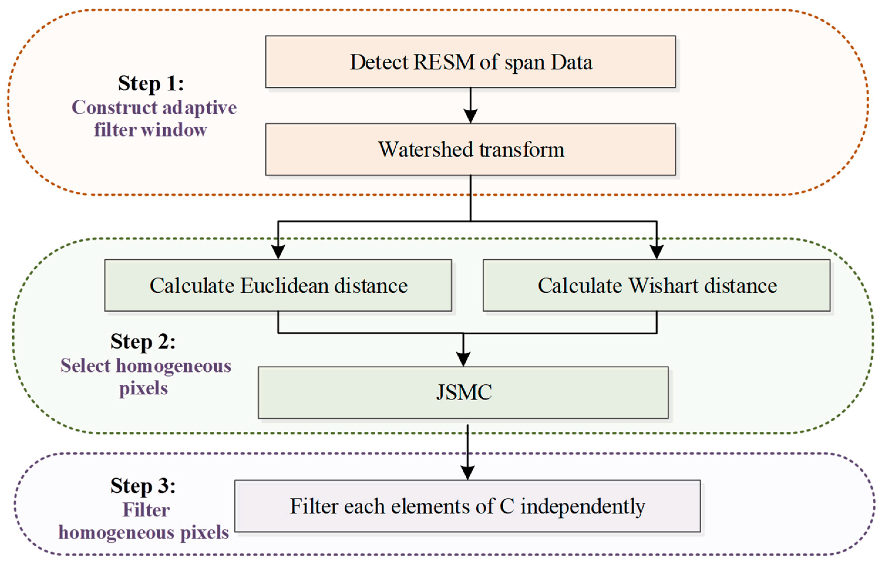
Based on the previous analysis, we present the complete flowchart of the JSMC filter in Figure 4. The JSMC filter mainly includes three steps.
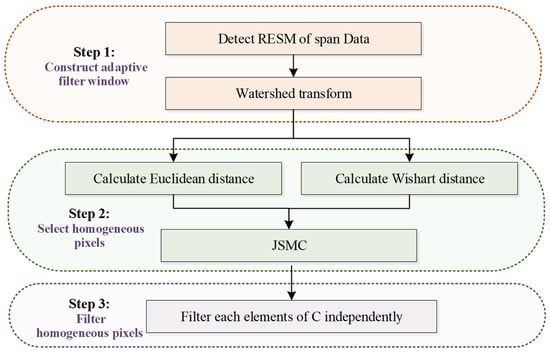
Figure 4.
Flowchart of PolSAR speckle filtering method based on JSMC.
STEP 1: Construct adaptive filter window.
Firstly, the multi-direction ratio edge detection is performed on the PolSAR span data. Secondly, the RESM of the PolSAR data is extracted by the threshold processing method. Finally, the watershed algorithm is utilized for the RESM in order to obtain the adaptive filtering windows. In the follow-up verification experiments of this paper, the parameters of the edge detector are set to: ,.
STEP 2: Select homogeneous pixels.
This step calculates the weighted Euclidean distance and Wishart distance of the pixel to be filtered and all pixels in the filter window and determines the joint similarity according to the JSMP. Next, JSMP will be sorted in descending order to select homogenous pixels that satisfy the conditions according to the set filter look.
STEP 3: Filter homogeneous pixels.
After the above steps are completed, the pixels satisfying the JSMC filter condition are filtered as the final pixel set. To preserve polarimetric properties, each element of the covariance matrix has to be filtered equally in a way similar to multi-look averaging.
3. Experiment Results
In this paper, the X-band airborne and C-band spaceborne PolSAR data are used for illustration. At the same time, the Re-Lee filter [9], IDAN filter [10], NLM filter [17] and JRP filter [15] are used to compare with the JSMC filter. Among them, the NLM filter is applied in a 21 × 21 searching window with a 7 × 7 patch, and the other three filters are applied with 7 × 7 pixel filter windows. By selecting the value of , the average window size of the JSMC filter is close to 49 pixels, which is similar to the size of the other 7 × 7 pixel windows.
3.1. Airborne Experiment
In this section, the polarization speckle filtering is performed on airborne PolSAR data. The data is collected by Xidian University and the Institute of Electronics at the Chinese Academy of Sciences (IECAS) in Meishan (Sichuan, CHN). Figure 5 shows the optical image and span image. The acquisition mode is X-band full-polarimetric Strip mode. The data is single-look complex (SLC) with a resolution of 0.2 m. The ground objects in the scene are mainly large dense shrub eucalyptus, well-distributed economic crop citrus, and grape. In order to clearly display the texture and other detailed information before and after filtering, the data in the red frame is intercepted for filtering. The intercepted data size is 1500 × 1500 pixels. The basic parameter information of the scene is shown in Table 1.
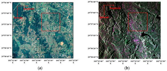
Figure 5.
Experimental scene in Meishan area, Sichuan. (a) Google Earth optical image; (b) span image of PolSAR data.

Table 1.
Parameters of Airborne PolSAR data.
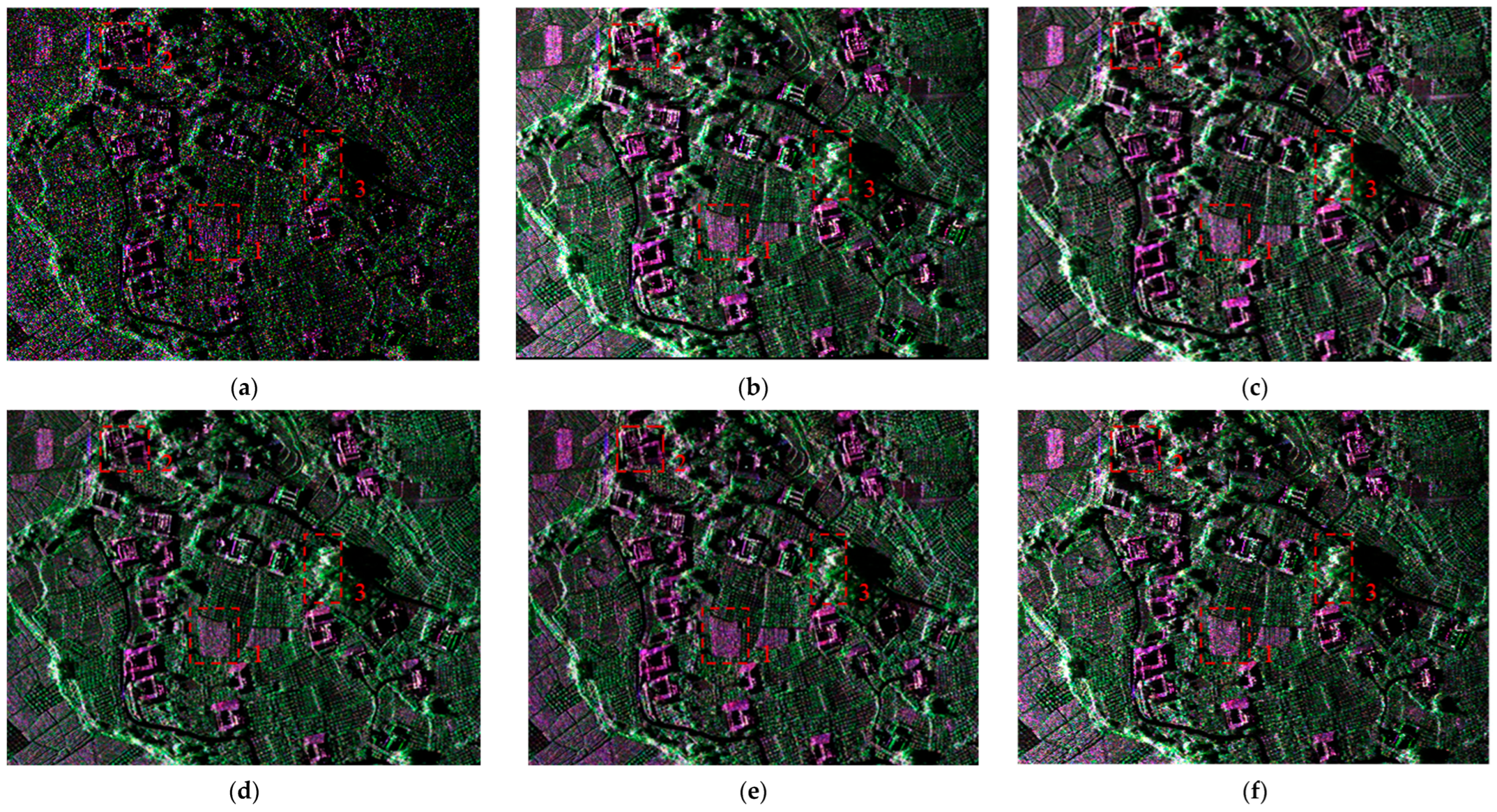
Figure 6 shows the Pauli decomposition results with the different filters. Figure 6a is the Pauli decomposition result of the SLC data. It can be seen that the SNR of the data is high. The contours between vegetation are clear, but the influence of speckle noise still exists. Figure 6b–f shows that all compared filters, as well as the JSMC filter, have a strong ability to suppress speckles. Next, we focus on region 1 of Figure 6 for a more detailed visual analysis.
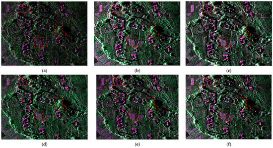
Figure 6.
The Pauli decomposition of different filters for Airborne PolSAR data cropped out from Figure 5. (a) Original Pauli image without filtering; (b) Re-Lee Filter; (c) IDAN Filter; (d) NLM Filter; (e) JRP Filter; (f) JSMC Filter.
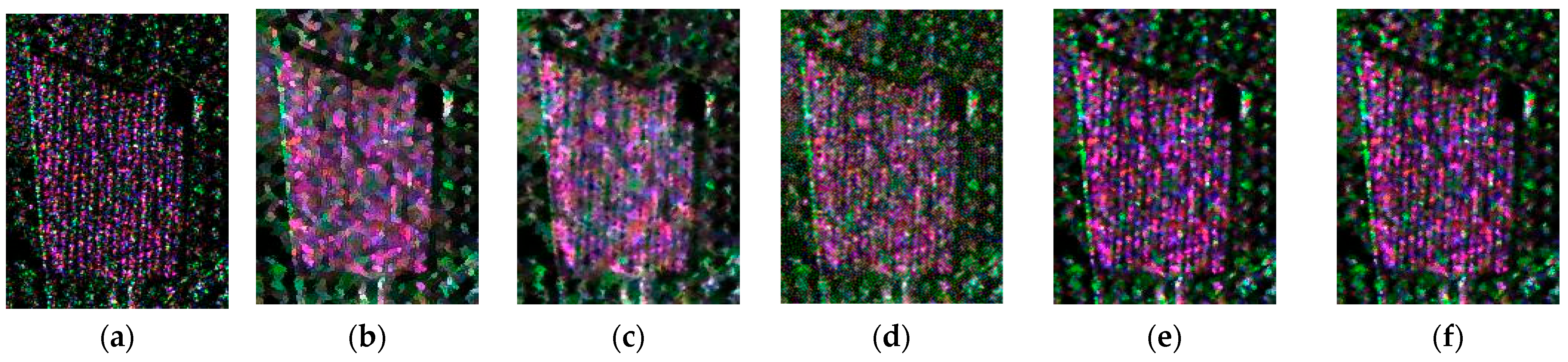
As shown in Figure 7, region 1 contains densely planted grapes. The row spacing between the grape crowns is about 0.6 m, and it spans about 3 pixels in the range direction of the SAR data. At this time, the scattering medium in the 7× 7 filtering window does not satisfy the local stationarity assumption, which brings great challenges to the filtering performance. Figure 7b shows the Pauli decomposition result filtered by a 7 × 7 Re-Lee filter. The result exhibits a good ability to reduce speckle. In particular, for the citrus trees in the upper right corner, the gap between canopy layers is still clearly visible after filtering. However, for denser grape vines, the canopy gaps are completely obscured. Both the IDAN filter and NLM filter in Figure 7d,e can retain the gaps between the grape vines to a certain extent, but the gaps are not particularly clear. Especially for the NLM filter, there is still residual speckle noise after filtering. For the JRP filter and JSMC filter, it can be seen from Figure 7d–f that the filters not only have a strong ability to remove speckle noise, but they can also better preserve the edge features of both the grape vines and the citrus trees.
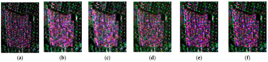
Figure 7.
The Pauli decomposition of different filters for region 1 in Airborne PolSAR data. (a) Original Pauli image without filtering; (b) Re-Lee Filter; (c) IDAN Filter; (d) NLM Filter; (e) JRP Filter; (f) JSMC Filter.
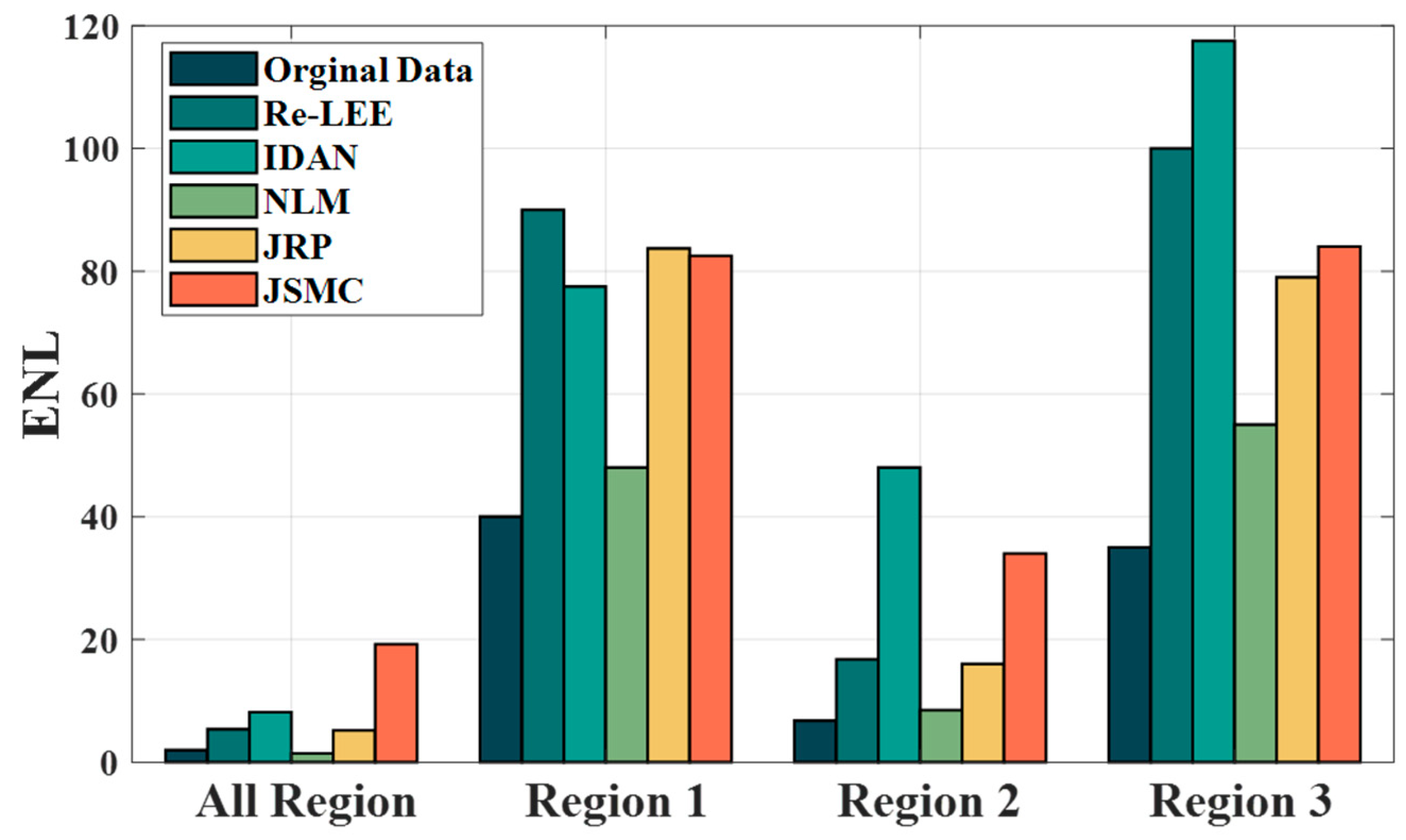
To further demonstrate the performance of the different filters, this paper employs two evaluation indicators for quantitative evaluation. One is the Equivalent Number of Looks (ENL) [28], and the other is the Edge Preserving Index (EPI) [29]. ENL is the ratio of mean square to variance of the distributed target intensity, defined as follows:
where, represents the mean value of the random variable, and represents the variance of the random variable. ENL characterizes the ability of the filter to smooth speckle noise in a homogeneous region. The larger the ENL, the more obvious the smoothing, and the better the effect of speckle suppression.
EPI is the ratio of the cumulative gradient changes in azimuth and range direction before and after filtering, and is defined as follows:
where, is the pixel value before filtering, and is the pixel value after filtering. The EPI indicates the retention degree of edge structure, and the value range is . The larger the EPI, the closer the filtered data is to the original data, and the stronger the edge preservation ability.
The ENLs and EPIs with different filters are recorded in Figure 8 and Figure 9. Regions 2 and 3 in Figure 8 and Figure 9 correspond to the positions marked by the red boxes in Figure 6, which are independent buildings and eucalyptus trees. Based on these indicators, we can conclude that the JSMC filter has better noise suppression performance and is significantly superior to the other four filters in terms of preserving edge structure.

Figure 8.
The ENL of Airborne PolSAR data filtered by different filters.
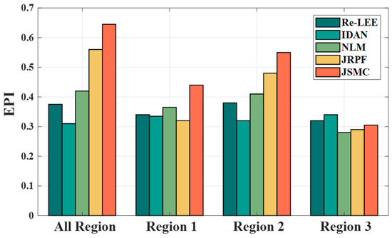
Figure 9.
The EPI of Airborne PolSAR data filtered by different filters.
Furthermore, this paper introduces the polarization scattering similarity factor (SSF) [30] to verify the ability to maintain polarization scattering characteristics. The SSF represents the retention degree of the polarization scattering mechanism. Assuming that the pixel before filtering is and the pixel after filtering is , the SSF is expressed as follows:
where the is the 2-norm of the vector. Obviously, the range of is . The larger the , the more similar the pixel is to pixel in the scattering mechanism. When , the polarization properties of the two pixels are identical. When , the two pixels are completely irrelevant. is the vector that includes all the elements of the covariance matrix, and it contains the polarization properties associated with the pixel, which can be expressed as:
The statistical curves of SSF under different filters are shown in Figure 10, respectively. It can be seen that the SSF curves of the IDAN filter are almost in superposition and their peaks are around 0.73, which is better than the Re-Lee filter. The curve for the NLM filter has a higher peak around 0.85, whereas the peak of the JRP and JSMC filters is near to 0.92 and the curve of JSMC filter is more concentrated, indicating that the proposed method can better maintain the polarization scattering characteristics.
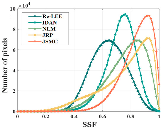
Figure 10.
Statistical curves of SSF for Airborne PolSAR data.
3.2. Spaceborne Experiment
In this section, the San Francisco (CA, USA) PolSAR data collected by the Gaofen-3 satellite is used to verify the performance of the filters in spaceborne data. The acquisition mode is C-band full-polarimetric Strip I (QPSI) mode. The data is SLC data with a resolution of 8 m. Figure 11 shows the Google Earth optical image and span image of the experimental scene. The scene includes oceans, vegetation, urban buildings, streets, etc. The buildings are regularly distributed with obvious texture features. In order to better display the details and texture, the scene in the red frame in Figure 11 will be intercepted for filtering. The intercepted data size is 1500 × 1500 pixels. The basic parameter information of the scene is shown in Table 2.
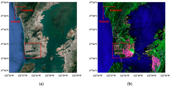
Figure 11.
Experimental scene in San Francisco, CA, USA. (a) Google Earth optical image; (b) span image of PolSAR data.
Table 2.
Parameters of Spaceborne PolSAR data.
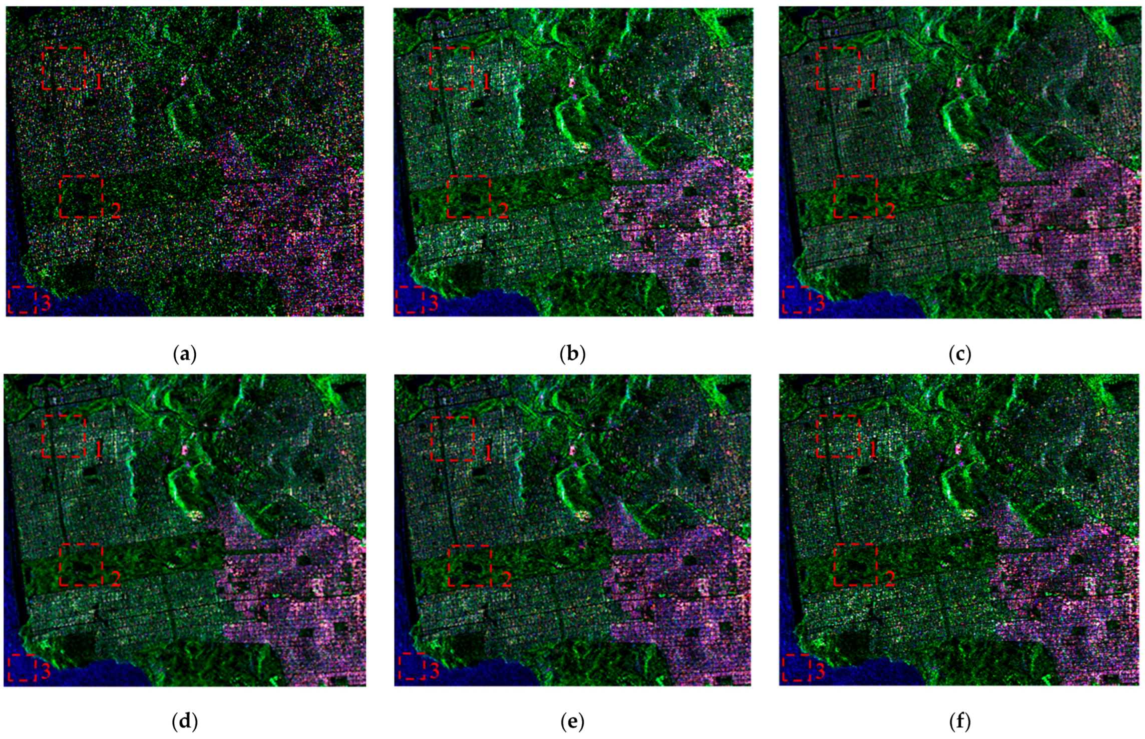
Figure 12a is the Pauli decomposition result of the SLC data. Figure 12b–f shows that the five filters all have certain speckle removal capabilities. We still intercept region 1 in Figure 12 for analysis filtering details. The results are shown in Figure 13.

Figure 12.
The Pauli decomposition of different filters for Spaceborne PolSAR data cropped out from Figure 11. (a) Original Pauli image without filtering; (b) Re-Lee Filter; (c) IDAN Filter; (d) NLM Filter; (e) JRP Filter; (f) JSMC Filter.

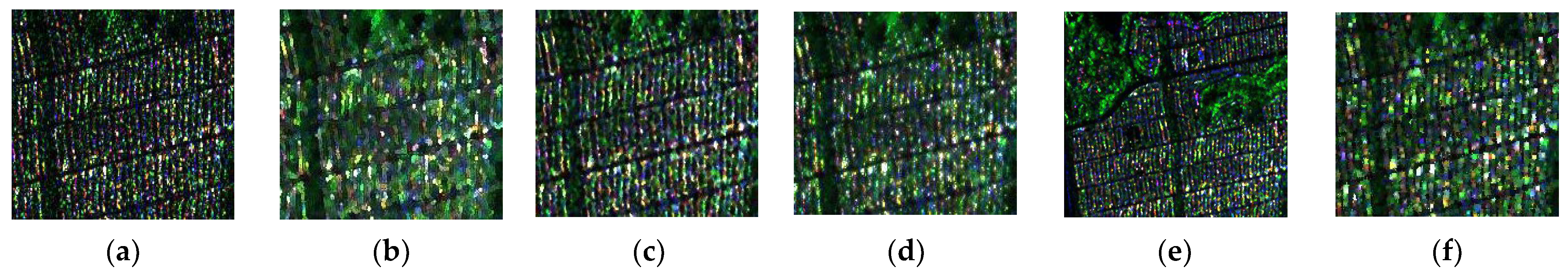
Figure 13.
The Pauli decomposition of different filters for region 1 in Spaceborne PolSAR data. (a) Original Pauli image without filtering; (b) Re-Lee Filter; (c) IDAN Filter; (d) NLM Filter; (e) JRP Filter; (f) JSMC Filter.
In Figure 13b,d, the result of the Re-Lee filter indicates that the filter is effective in speckle suppression, but there is still visible blurring in densely built-up areas. In Figure 13c,e, while the IDAN and JRP filters clearly highlight the texture of the buildings, their data smoothing effect are relatively subpar.
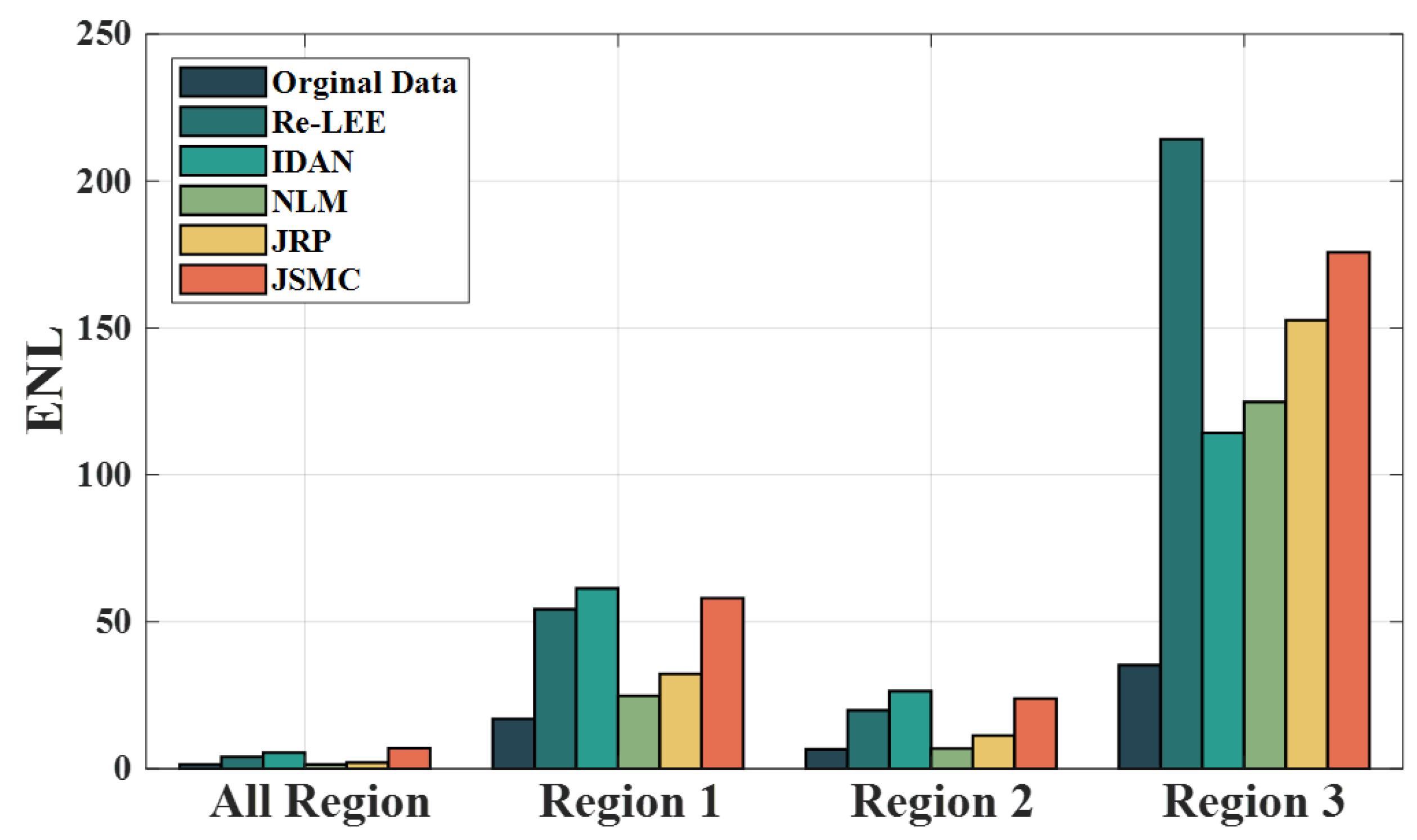
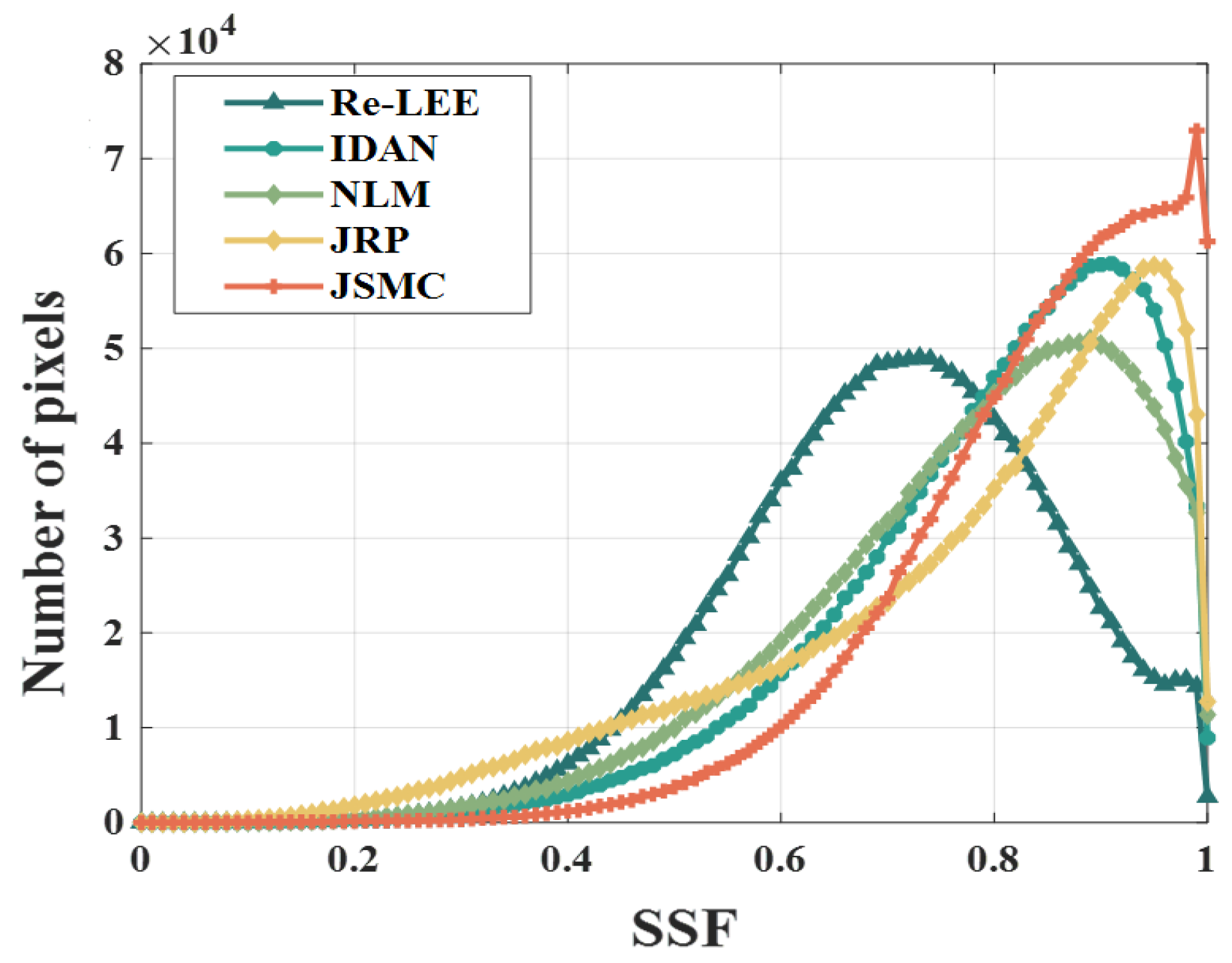
Figure 14 and Figure 15 show the comparison results of ENL and EPI for different filters, while Figure 16 presents the statistical curve of SSF for different filters. Through the above analysis, it can be summarized that the JSMC filter is still capable of perfect edge structure preservation, excellent speckle suppression, and the best preservation of polarization scattering properties in spaceborne PolSAR data.

Figure 14.
The ENL of Spaceborne PolSAR data filtered by different filters.
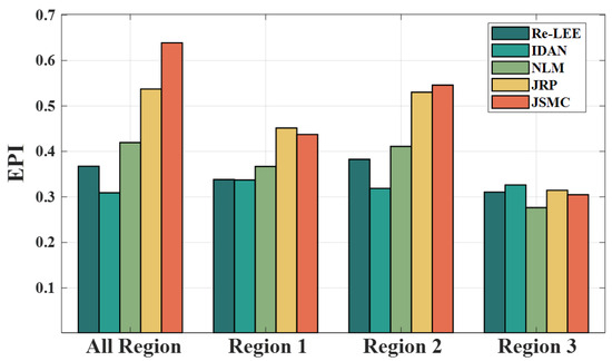
Figure 15.
The EPI of Spaceborne PolSAR data filtered by different filters.
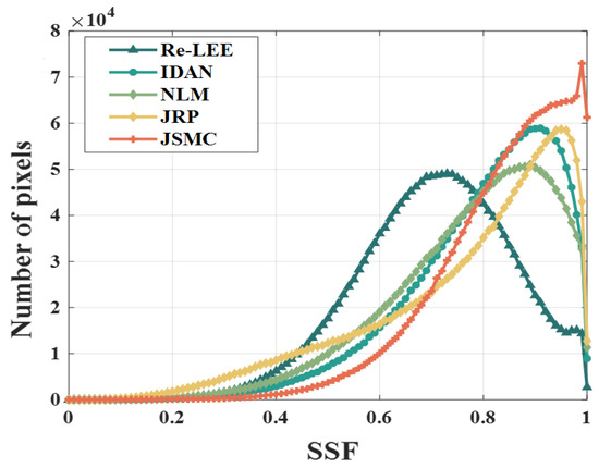
Figure 16.
Statistical curves of SSF for Spaceborne PolSAR data.
4. Discussion
For high-resolution PolSAR data, different scattering media in vegetation and urban areas, such as gaps in the canopy, break the assumption of local stationarity and reduce the performance of traditional filters. This presents a challenge in selecting homogeneous regions for speckle filtering in the spatial domain. To address the issue, this paper proposes a new PolSAR speckle filter called a JSMC filter. The filter utilizes an adaptive adjustment factor based on (9) to determine the initial size of the adaptive filtering window. This process resembles super-pixel segmentation but differs from algorithms such as Simple Linear Iterative Clustering (SLIC) [31]. Instead of using pixel clustering to determine homogeneous regions, our algorithm utilizes rotated rectangular windows for edge detection within these regions. This approach effectively minimizes the impact of speckle noise on window construction. Figure 2 shows that the JSMC filter has higher edge detection accuracy and structure preservation capability. Additionally, the filter is based on JSMC in order to measure the similarity between polarimetric covariance matrices and thus select homogeneous pixels. In dealing with the unavoidable existence of non-homogeneous pixels in irregular windows, our algorithm utilizes JSMC for selection in order to guarantee homogeneity among the filtering pixels. Figure 6, Figure 7, Figure 8, Figure 9, Figure 12, Figure 13, Figure 14 and Figure 15 demonstrate the superiority of the JSMC filter for speckle suppression on airborne and spaceborne PolSAR data. Moreover, the JSMC filter demonstrates excellent capability in preserving the edges of vegetation and building gaps, while also maintaining the polarimetric performance.
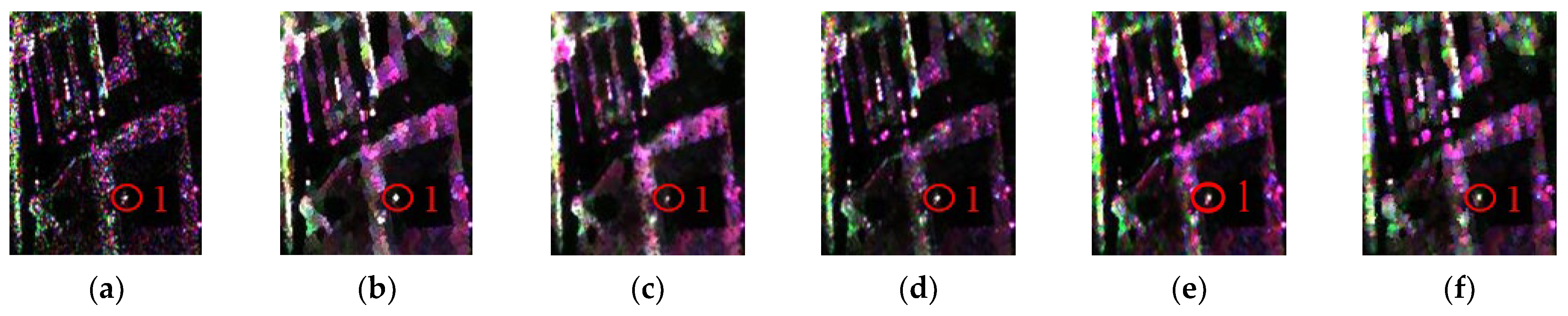
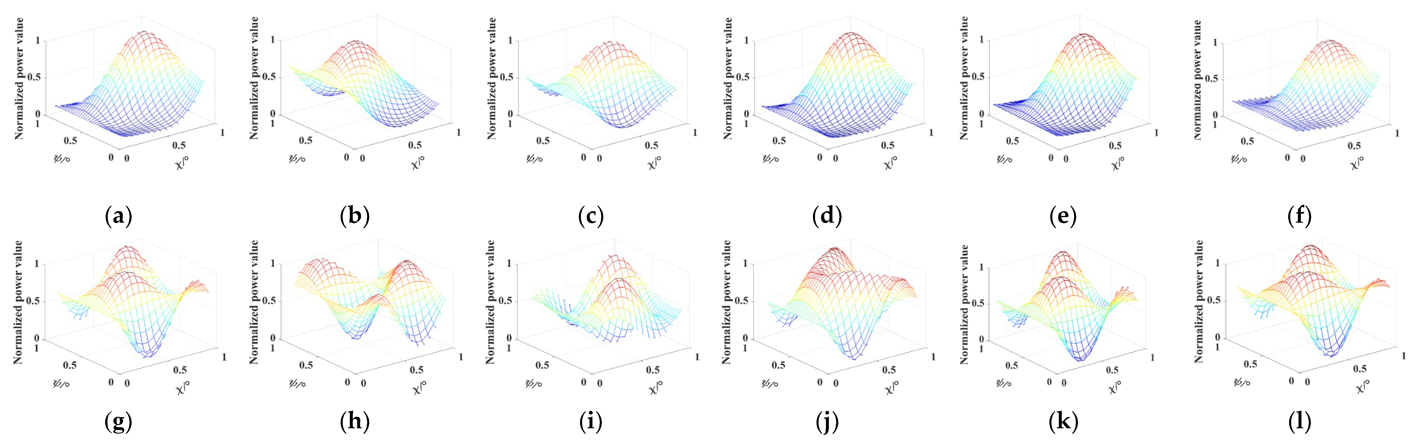
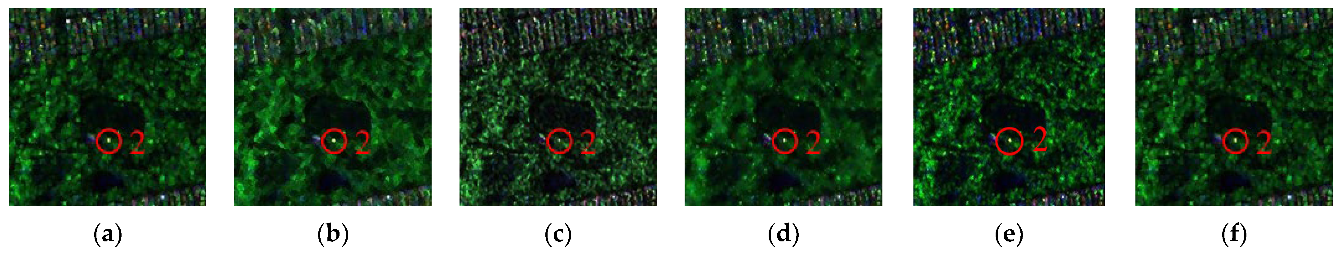
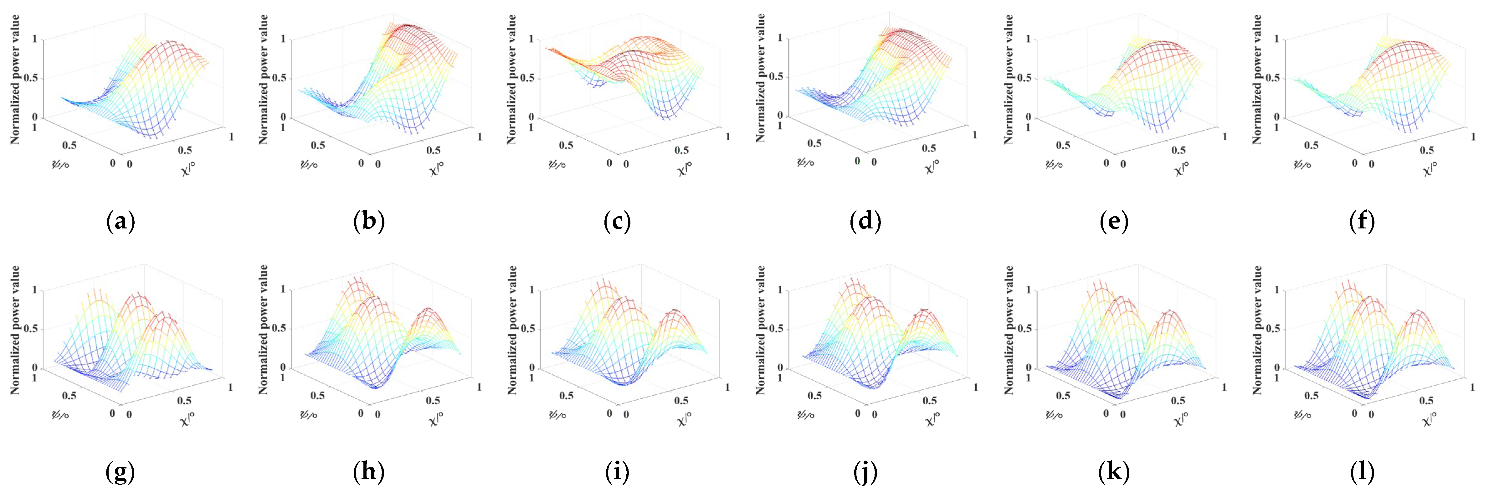
Additionally, two strong targets are selected in the building area of the airborne data and the vegetation area of the spaceborne data to explore their polarimetric responses, which are formed in a combination of ellipse orientation angle (degree) and ellipticity angle (degree). Theoretically, the polarization response shape of strong scatterers should stay the same before and after filtering. Figure 17 shows the Pauli decomposition results of region 2 in Figure 6 with different filters. Figure 18 shows the polarization response of pixel (132, 25) in Figure 17. Figure 19 shows the Pauli decomposition results of region 2 in Figure 12 with different filters. Figure 20 shows the polarization response of pixel (58, 97) in Figure 19.
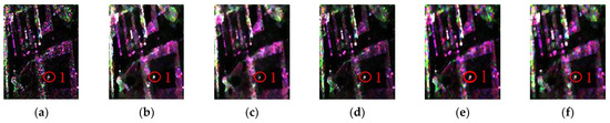
Figure 17.
The Pauli decomposition of different filters for region 2 in Figure 6. (a) Original Pauli image; (b) Re-Lee Filter; (c) IDAN Filter; (d) NLM Filter; (e) JRP Filter; (f) JSMC Filter.
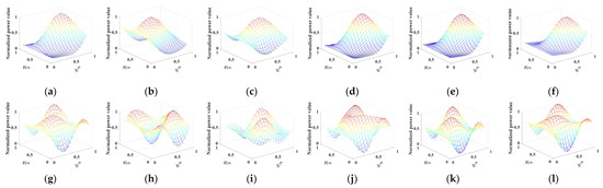
Figure 18.
Co-polarized and cross-polarized signatures of (132, 25) pixel in Figure 6. (a,g) Original signatures without filtering; (b,h) Re-Lee Filter; (c,i) IDAN Filter; (d,j) NLM Filter; (e,k) JRP Filter; (f,l) JSMC Filter.
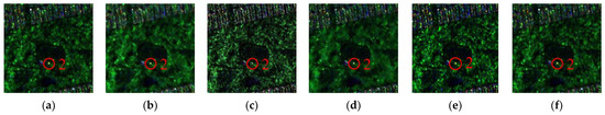
Figure 19.
The Pauli decomposition of different filters for region 2 in Figure 12. (a) Original Pauli image without filtering; (b) Re-Lee Filter; (c) IDAN Filter; (d) NLM Filter; (e) JRP Filter; (f) JSMC Filter.

Figure 20.
Co-polarized and cross-polarized signatures of (58, 97) pixel in Figure 19. (a,g) Original signatures without filtering; (b,h) Re-Lee Filter; (c,i) IDAN Filter; (d,j) NLM Filter; (e,k) JRP Filter; (f,l) JSMC Filter.
Compared to the original data, the Re-Lee and the IDAN filter produce polarimetric responses with significant differences in shape trend. The NLM and JRP filters have similar co-polarization responses to the true response, but distinctions still exist in the cross-polarization responses. For the JSMC filter, both the co-polarization and cross-polarization responses are consistent with the true response.
5. Conclusions
Scattering noise is an inherent phenomenon in PolSAR data. It is caused by the coherent summation of multiple scattering echoes from scatterers. To improve the processing accuracy of polarimetric data, the polarimetric covariance or coherence matrix is usually obtained through second-order statistics of spatially neighboring pixels. This process is called PolSAR speckle filtering. However, for high-resolution SAR data, the pixels within a 7 × 7 or even a 3 × 3 window may not be homogeneous. Therefore, this paper proposes a PolSAR speckle filter based on JSMC. The filter constructs the scale-adaptive filtering window to adapt different edge structures and textures present in the scene. It utilizes a multi-directional ratio edge detector to detect edges and determine the appropriate size of the filtering window. This adaptive approach enables the preservation of fine details and texture while effectively reducing speckle. Additionally, the JSMC filter addresses the challenge of non-homogeneity in high-resolution SAR data. It recognizes that, within a small window, the pixels may exhibit significant variations in their scattering properties. To this end, JSMC is proposed in this paper. Based on JSMC, a filter can select homogeneous pixels that share similar scattering characteristics, ensuring stable filtering of the PolSAR data. The effectiveness of the proposed filter is validated utilizing X-band airborne data and C-band spaceborne data, and compared with a classical Re-Lee filter, IDAN filter, NLM filter, and JRP filter. The experimental results demonstrate that the proposed filter outperforms these filters in terms of morphology preservation, scattering mechanism preservation, and speckle suppression.
Author Contributions
Conceptualization, F.T., Z.L. and Q.Z.; methodology, F.T. and Z.S.; software, F.T.; validation, F.T., C.X. and H.G.; formal analysis, F.T.; investigation, Z.Z.; resources, F.T.; data curation, F.T. and H.G.; writing—original draft preparation, F.T.; writing—review and editing, F.T., Z.L., Z.S., Z.Z. and C.X.; visualization, F.T. and H.G.; supervision, Z.L.; project administration, F.T.; funding acquisition, F.T. All authors have read and agreed to the published version of the manuscript.
Funding
This research was funded by the National Natural Science Foundation of China under grant number 62031005.
Data Availability Statement
Not applicable.
Conflicts of Interest
The authors declare no conflict of interest.
References
- Lee, J.S.; Pottier, E. Polarimetric Radar Imaging: From Basics to Applications; CRC Press: Boca Raton, FL, USA, 2017. [Google Scholar]
- Lu, H.; Zhao, J.; Zheng, B.; Qian, C.; Cai, T.; Li, E.; Chen, H. Eye accommodation-inspired neuro-metasurface focusing. Nat. Commun. 2023, 14, 3301. [Google Scholar] [CrossRef] [PubMed]
- Lee, J.S.; Grunes, M.R.; Ainsworth, T.L.; Du, L.J.; Schuler, D.L.; Cloude, S.R. Unsupervised classification using polarimetric decomposition and the complex Wishart classifier. IEEE Trans. Geosci. Remote Sens. 1999, 37, 2249–2258. [Google Scholar]
- Lee, J.S.; Grunes, M.R.; De Grandi, G. Polarimetric SAR speckle filtering and its implication for classification. IEEE Trans. Geosci. Remote Sens. 1999, 37, 2363–2373. [Google Scholar]
- Cloude, S.R.; Corr, D.G.; Williams, M.L. Target detection beneath foliage using polarimetric synthetic aperture radar interferometry. Waves Random Media 2004, 14, S393. [Google Scholar] [CrossRef]
- Sletten, M.; Brozena, J. Detection of targets beneath foliage using aspect-angle variation of the polarimetric SAR response. In Proceedings of the 2014 IEEE Radar Conference, Cincinnati, OH, USA, 19–23 May 2014; pp. 0296–0297. [Google Scholar]
- Novak, L.M.; Burl, M.C. Optimal speckle reduction in polarimetric SAR imagery. In Proceedings of the Twenty-Second Asilomar Conference on Signals, Systems and Computers, Pacific Grove, CA, USA, 31 October–2 November 1988; Volume 2, pp. 781–793. [Google Scholar]
- Lee, J.S.; Hoppel, K.; Mango, S.A. Unsupervised estimation of speckle noise in radar images. Int. J. Imaging Syst. Technol. 1992, 4, 298–305. [Google Scholar] [CrossRef]
- Lee, J.S. Digital image enhancement and noise filtering by use of local statistics. IEEE Trans. Pattern Anal. Mach. Intell. 1980, 2, 165–168. [Google Scholar] [CrossRef]
- Vasile, G.; Trouvé, E.; Lee, J.S.; Buzuloiu, V. Intensity-driven adaptive-neighborhood technique for polarimetric and interferometric SAR parameters estimation. IEEE Trans. Geosci. Remote Sens. 2006, 44, 1609–1621. [Google Scholar] [CrossRef]
- D’Hondt, O.; Lopez-Martinez, C.; Ferro-Famil, L.; Pottier, E. Spatially nonstationary anisotropic texture analysis in SAR images. IEEE Trans. Geosci. Remote Sens. 2007, 45, 3905–3918. [Google Scholar] [CrossRef]
- Lopez-Martinez, C.; Fabregas, X. Model-based polarimetric SAR speckle filter. IEEE Trans. Geosci. Remote Sens. 2008, 46, 3894–3907. [Google Scholar] [CrossRef]
- Guo, R.; Liu, Y.; Zang, B.; Xing, M. A Polarimetric SAR Image Filtering Method Preserving Scattering Properties. J. Xidian Univ. 2011, 38, 90–95. [Google Scholar]
- Wu, Z.; Ouyang, Q.; Hu, Z.; Liu, L. Application of four-component scattering model in speckle filtering for polarimetric SAR. J. Wuhan Univ. Inf. Sci. Ed. 2011, 36, 763–766. [Google Scholar]
- Xie, J.; Li, Z.; Zhou, C.; Fang, Y.; Zhang, Q. Speckle filtering of GF-3 polarimetric SAR data with joint restriction principle. Sensors 2018, 18, 1533. [Google Scholar] [CrossRef] [PubMed]
- Deledalle, C.A.; Denis, L.; Tupin, F. Iterative weighted maximum likelihood denoising with probabilistic patch-based weights. IEEE Trans. Image Process. 2009, 18, 2661–2672. [Google Scholar] [CrossRef] [PubMed]
- Deledalle, C.A.; Denis, L.; Tupin, F.; Reigber, A.; Jäger, M. NL-SAR: A unified nonlocal framework for resolution-preserving (Pol)(In) SAR denoising. IEEE Trans. Geosci. Remote Sens. 2014, 53, 2021–2038. [Google Scholar] [CrossRef]
- Wu, J.; Liu, F.; Hao, H.; Li, L.; Jiao, L.; Zhang, X. A nonlocal means for speckle reduction of SAR image with multiscale-fusion-based steerable kernel function. IEEE Geosci. Remote Sens. Lett. 2016, 13, 1646–1650. [Google Scholar] [CrossRef]
- Sharifymoghaddam, M.; Beheshti, S.; Elahi, P.; Hashemi, M. Similarity validation based nonlocal means image denoising. IEEE Signal Process. Lett. 2015, 22, 2185–2188. [Google Scholar] [CrossRef]
- Shen, P.; Wang, C.; Gao, H.; Zhu, J. An adaptive nonlocal mean filter for PolSAR data with shape-adaptive patches matching. Sensors 2018, 18, 2215. [Google Scholar] [CrossRef]
- Burger, H.C.; Schuler, C.J.; Harmeling, S. Image denoising: Can plain neural networks compete with BM3D? In Proceedings of the 2012 IEEE Conference on Computer Vision and Pattern Recognition, Providence, RI, USA, 16–21 June 2012; pp. 2392–2399. [Google Scholar]
- Chierchia, G.; Cozzolino, D.; Poggi, G.; Verdoliva, L. SAR image despeckling through convolutional neural networks. In Proceedings of the 2017 IEEE International Geoscience and Remote Sensing Symposium (IGARSS), Fort Worth, TX, USA, 23–28 July 2017; pp. 5438–5441. [Google Scholar]
- Mullissa, A.G.; Persello, C.; Reiche, J. Despeckling polarimetric SAR data using a multistream complex-valued fully convolutional network. IEEE Geosci. Remote Sens. Lett. 2021, 19, 4011805. [Google Scholar] [CrossRef]
- Lee, J.S.; Wen, J.H.; Ainsworth, T.L.; Chen, K.S.; Chen, A. Improved sigma filter for speckle filtering of SAR imagery. IEEE Trans. Geosci. Remote Sens. 2008, 47, 202–213. [Google Scholar]
- Lopes, A.; Touzi, R.; Nezry, E. Adaptive speckle filters and scene heterogeneity. IEEE Trans. Geosci. Remote Sens. 1990, 28, 992–1000. [Google Scholar] [CrossRef]
- Donoho, D.L. De-noising by soft-thresholding. IEEE Trans. Inf. Theory 1995, 41, 613–627. [Google Scholar] [CrossRef]
- Schou, J.; Skriver, H.; Nielsen, A.A.; Conradsen, K. CFAR edge detector for polarimetric SAR images. IEEE Trans. Geosci. Remote Sens. 2003, 41, 20–32. [Google Scholar] [CrossRef]
- Foucher, S.; López-Martínez, C. Analysis, evaluation, and comparison of polarimetric SAR speckle filtering techniques. IEEE Trans. Image Process. 2014, 23, 1751–1764. [Google Scholar] [CrossRef] [PubMed]
- Di Martino, G.; Poderico, M.; Poggi, G.; Riccio, D.; Verdoliva, L. Benchmarking framework for SAR despeckling. IEEE Trans. Geosci. Remote Sens. 2013, 52, 1596–1615. [Google Scholar] [CrossRef]
- Wang, Y.; Yang, J.; Li, J. Similarity-intensity joint PolSAR speckle filtering. In Proceedings of the 2016 CIE International Conference on Radar (RADAR), Guangzhou, China, 10–13 October 2016; pp. 1–5. [Google Scholar]
- Liu, P.; Li, Z.; Lou, L.; Yang, W.; Wang, Z. Layover and shadow regions detection based on superpixel segmentation and multi-information fusion. Acta Geod. Cartogr. Sin. 2022, 51, 2517–2530. [Google Scholar]


Disclaimer/Publisher’s Note: The statements, opinions and data contained in all publications are solely those of the individual author(s) and contributor(s) and not of MDPI and/or the editor(s). MDPI and/or the editor(s) disclaim responsibility for any injury to people or property resulting from any ideas, methods, instructions or products referred to in the content. |
© 2023 by the authors. Licensee MDPI, Basel, Switzerland. This article is an open access article distributed under the terms and conditions of the Creative Commons Attribution (CC BY) license (https://creativecommons.org/licenses/by/4.0/).