Abstract
Using Global Navigation Satellite Systems (GNSS) observation data for developing a high-precision ionospheric Total Electron Content (TEC) model is one of the essential subjects in ionospheric physics research and the application of satellite navigation correction. In this study, we integrate the Empirical Orthogonal Function (EOF) method with the TEC data provided by the Center for Orbit Determination in Europe (CODE), and observed by the dense GNSS receivers operated by the Crustal Movement Observation Network of China (CMONOC) to construct a regional ionospheric TEC model over China. The EOF analysis of CODE TEC in China from 1998 to 2010 shows that the first-order EOF component accounts for 90.3813% of the total variation of the ionospheric TEC in China. Meanwhile, the average value of CODE TEC is consistent with the spatial and temporal distribution characteristics of the first-order EOF base function, which mainly reflects the latitude and diurnal variations of TEC in China. The first-order coefficient after EOF decomposition shows an obvious 11-year period and semi-annual variations. The maximum amplitude of semi-annual variation mainly appears in March and October, which is closely associated with the variation in geographical longitude, the semi-annual change of the low-latitude electric field, and the ionospheric fountain effect. The second-order coefficient has an evident annual variation, the minimum amplitude mainly occurs in March, August, and September, and the amplitude values in the high solar activity years are more significant than those in the low solar activity years. The third-order coefficient mainly shows the characteristics of annual variation, and the fourth-order coefficient shows the noticeable semi-annual and annual variations. The third and fourth-order coefficients are both modulated by the solar activity index F10.7. The ionospheric TEC model in China, driven by CMONOC real-time GNSS observation data, can better reflect the latitude, local time and seasonal variation characteristics of ionospheric TEC over China. In particular, it can clearly show the spring and autumn asymmetry of ionospheric TEC in the low latitudes. The root mean square error of the absolute error between the model and the actual observation is mainly distributed around 2.45 TECU (1 TECU = 1016 electrons/m2). The values of the TEC model constructed in this study are closer to the actual observed values than those of the CODE TEC in China.
1. Introduction
The total electron content (TEC) is a key parameter for studying the morphology, structure, and change of the ionosphere [1,2,3]. With the continuous development of Global Navigation Satellite Systems (GNSS), GNSS provides an opportunity to efficiently detect ionospheric TEC [4,5,6]. How to use GNSS data to construct the high-precision ionospheric TEC model has traditionally been one of the focal issues in the research fields of ionospheric physics and geodetic surveying.
At present, the methods of constructing regional ionospheric TEC model using GNSS data mainly include trigonometric series, polynomial, spherical cap harmonic, spherical harmonic function, empirical orthogonal function (EOF), and so on [7,8,9,10,11,12,13,14]. The EOF decomposition is a classical data analysis and modeling method. The most important feature of this method is that the base function is not given artificially in advance, but is naturally generated by the observation data itself during the calculation process, which can better reflect the characteristics of the inherent variation in the data and demonstrates a good convergence speed [15,16]. Based on the characteristics of the EOF method, in recent years, some scholars have applied this method to analyze the ionospheric observation data [17,18,19,20,21,22,23,24,25,26,27]. Zhao et al. [17] applied the EOF method for a statistical analysis of the total ion density in the topside ionosphere from 1996 to 2004. The analysis results indicate that extreme ultraviolet radiation is the major factor in controlling the change of the total ion density in the topside ionosphere. Zhang et al. [28] conducted an analysis of the TEC data over North America during 2001–2012 by the EOF method. The results demonstrate that the first-order EOF component mainly reflects the average state of ionospheric TEC, and the second-order EOF component reflects the effect of geomagnetic declination in the mid-latitude ionosphere. Based on the Global Ionosphere Map (GIM) data of the Jet Propulsion Laboratory (JPL) for about 15 years, Yao et al. [29] compared and analyzed the variation characteristics of ionospheric TEC in East Asia and North America using the EOF method, and pointed out that the variation characteristics of the first three components in the two regions are in good agreement. Chen et al. [30] utilized the EOF method to analyze the spatial and temporal variations of TEC in North America. They verified the EOF method’s effectiveness in data analysis.
In the modeling by the EOF method, Liu et al. and Zhang et al. [18,19] utilized the EOF method to construct single-station and global empirical models for the ionospheric propagation factor M(3000)F2. A single-station empirical model of foF2 was constructed using the EOF method and the observational data of three ionosonde stations in Japan from 1971 to 1987 [31]. The results show that the first-order EOF coefficient mainly reflects the characteristics of the components with solar cycle, annual, and semi-annual variation. Based on the EOF method, Yu et al. [32] constructed the empirical models of ionospheric foF2, M(3000)F2, hmF2, and foE over China by 24-ionosonde observations and adjacent areas from 1964 to 1976. Based on multiple TEC observation data and the International Reference Ionosphere (IRI) 2012 model, She et al. [24] combined the spherical harmonic function and EOF method to construct a global model for ionospheric electron density. The model results are closer to the observed results than those of the IRI-2012 model. Some scholars have constructed climatological models of TEC in Wuhan and China using the EOF method and observational data from the Wuhan station and the Crustal Movement Observation Network of China (CMONOC) [33,34]. Utilizing JPL-GIM data from 1998 to 2010, Wan et al. [35] constructed a global ionospheric empirical model of TEC using the EOF method and spherical harmonic function. This model can accurately reflect the temporal and spatial variations of the global ionospheric TEC. Based on the GIM data of the international GNSS service, Li et al. [36] extracted the spatial and diurnal variation characteristics of the ionospheric TEC over China and adjacent areas from 2007 to 2016 through a two-layer EOF analysis. The EOF-based model can demonstrate temporal and spatial variation characteristics of ionospheric TEC and obtain minor modeling errors more effectively than the IRI-2016.
The continuous increase of GNSS observational data in China provides an opportunity for constructing a regional ionospheric TEC model over China with high spatial and temporal resolution and high precision. In this paper, we intend to use the TEC data of the Center for Orbit Determination in Europe (CODE) to analyze the spatial and temporal variation characteristics of ionospheric TEC in China by the EOF method [37,38]. On this basis, the dense GNSS observation data in China are used as a driving source to construct a regional ionospheric TEC model over China.
2. Data and Methods
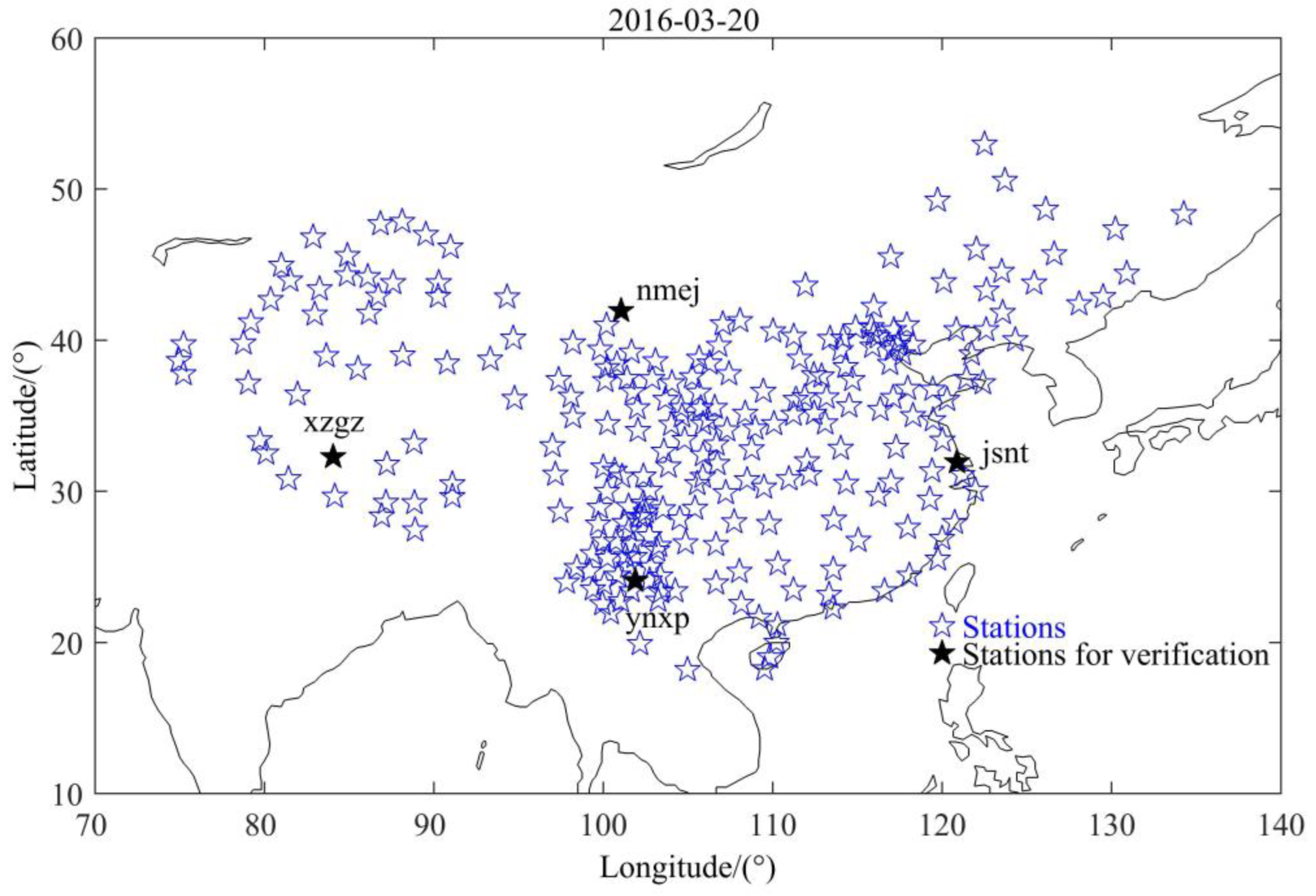
The data used for this study include the CODE TEC GIMs from 2 June 1998 to 31 December 2010, with spatial ranges of 10°S~60°N and 60°E~150°E. The CODE GIM is a global TEC product with resolutions of 5° × 2.5° × 2 h (longitude × latitude × Universal Time), which is interpolated 1 h in the time resolution between 00:00 and 23:00 Universal Time (UT) in this study. The TEC at the Ionospheric Pierce Point (IPP) is retrieved from the Receiver Independent Exchange Format files recorded by the dense ground-based GNSS receivers operated by the CMONOC [39]. The TEC data are at a time resolution of 30 s and in units of TECU (1 TECU = 1016 electrons/m2). The corresponding retrieving method of TEC can refer to the relevant literature [37,40]. Figure 1 shows the distribution of CMONOC GNSS stations on 20 March 2016, where the black pentagram indicates the stations that did not participate in the modeling during the model accuracy test. In addition, the TEC with a time resolution of 1 h in 2016 released by CODE is used for comparative analysis and error test of the model.
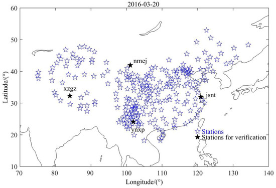
Figure 1.
Distribution of CMONOC’s GNSS stations on 20 March 2016.
The EOF method is used for the analysis and modeling of the ionospheric TEC in this study, which is expressed as:
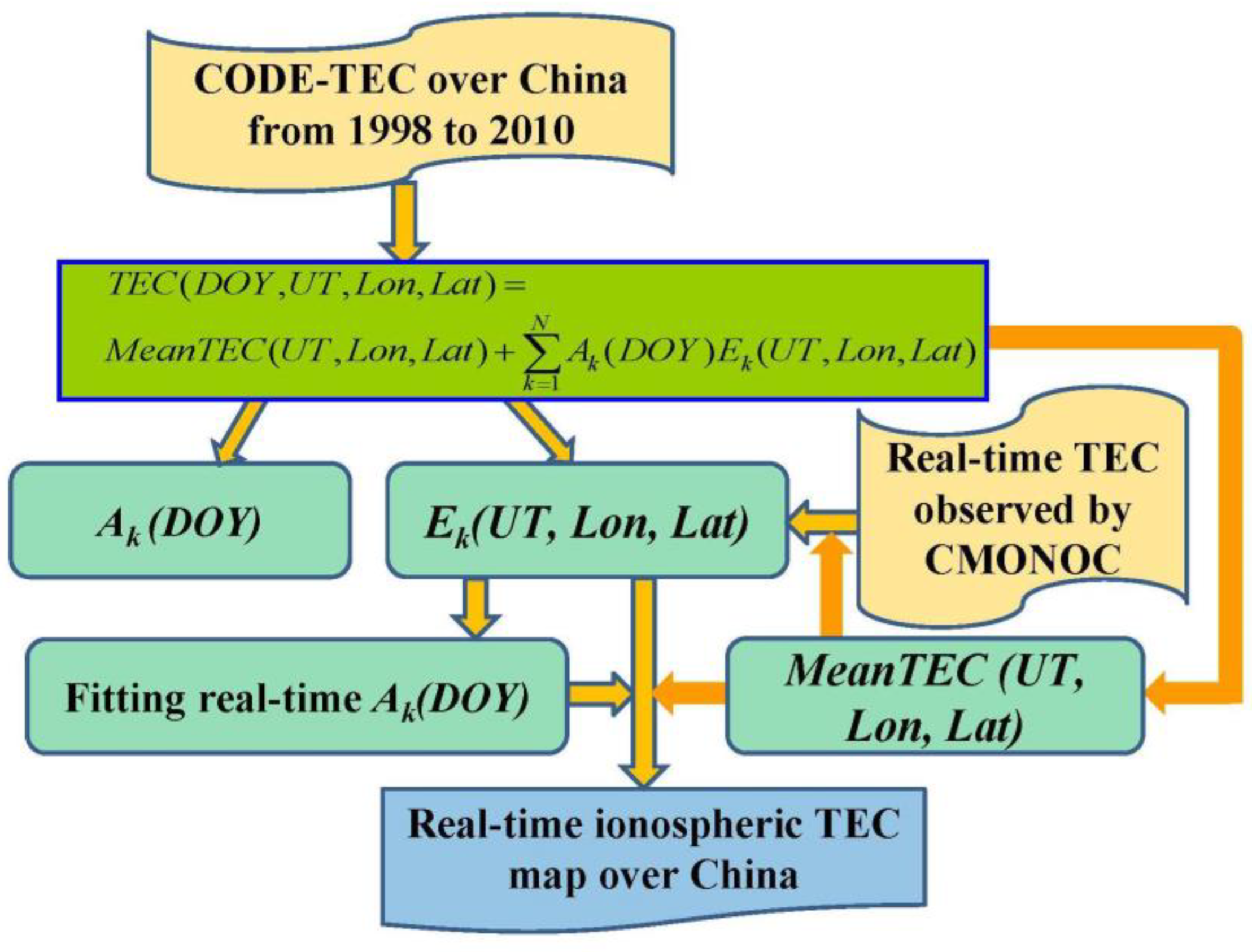
Here, TEC is the vertical TEC at the IPPs, which varies with DOY, UT, Lon, and Lat. DOY is the date number of a year, UT is the Universal Time, Lon is the geographical longitude, Lat is the geographical latitude, mean TEC is the average vertical TEC on UT, Lon, and Lat. K is the order, N is the maximum value of the order, Ak and Ek indicate the coefficients and the orthogonal basic functions after EOF decomposition, respectively. In the process of constructing the ionospheric TEC model over China, the CODE TEC data over China from 1998 to 2010 are used to take the average value according to UT, Lon, and Lat. Then, the CODE TEC is used to subtract the average value, and then the CODE TEC without mean TEC is decomposed into the sum of the product of the coefficient and the base function by the EOF method. The coefficient part mainly reflects the change with DOY, and the base function part mainly reflects the variations with UT, Lon, and Lat. After the EOF decomposition of the historical CODE TEC from 1998 to 2010, some order base functions are selected and combined with the real-time TEC data observed by CMONOC dense stations in China to fit the real-time coefficients. In the process of fitting the real-time coefficients, we first select the TEC observation data of CMONOC from the first 15 min to the current time, and use the historical average values and base function values to interpolate the corresponding average values and base function values on the UT, longitude, and latitude of the selected TEC data from CMONOC. With the TEC from CMONOC, the interpolated average values, and the interpolated base function values, we use least squares fitting to get the real-time coefficients by Formula (1). To obtain the real-time coefficient A, we use only 15 min of data instead of a full day’s data. Therefore, the obtained coefficient will vary with UT. Finally, the real-time ionospheric TEC model in China is constructed by combining the real-time coefficients with the historical base functions and TEC average values. Figure 2 illustrates the specific modeling process.

Figure 2.
Flow chart of real-time TEC model construction in China.
3. Results
3.1. Results of EOF Decomposition of CODE TEC
Based on the TEC modeling process in Figure 2, an EOF decomposition is performed on the CODE TEC data in China from 1998 to 2010. Table 1 gives the distributions of contribution and cumulative contribution rates for the first 16-order coefficients and base functions resulting from the EOF decomposition of the CODE TEC without mean TEC. Table 1 indicates that the first-order EOF component accounts for 90.3813% of the total variation of TEC, the cumulative contribution rate of the first to third-order EOF components accounts for 95.0358% of the total variation of TEC, and the contribution rate of the 14th and above orders to the total variation of TEC is less than 0.1000%. To perform further analysis of the variation features of base functions and coefficients in different EOF components, Figure 3, Figure 4 and Figure 5 show the distributions of the mean value of CODE TEC and the first to third-order EOF-decomposed base functions with latitude and longitude for the periods of 00:00, 06:00, and 12:00 UT in China from 1998 to 2010, respectively. Figure 6 demonstrates the distributions of the solar activity index F10.7 and the first to fourth-order coefficients derived from the EOF decomposition of the CODE TEC in China from 1998 to 2010.

Table 1.
The distributions of contribution and cumulative contribution rates for the first 16 EOF components derived from the CODE TEC without mean TEC.
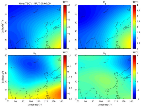
Figure 3.
The spatial distributions of the mean TEC and the first three EOF modes derived from CODE TEC in China from 1998 to 2010 at 00:00 UT.
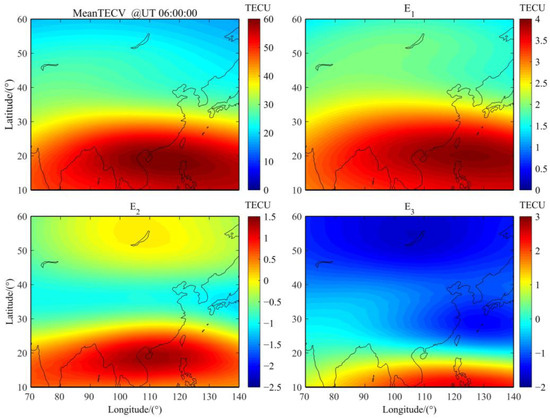
Figure 4.
The spatial distributions of the mean TEC and the first three EOF modes derived from CODE TEC in China from 1998 to 2010 at 06:00 UT.
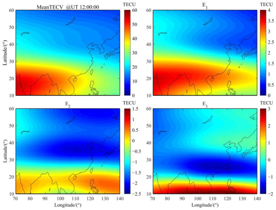
Figure 5.
The spatial distributions of the mean TEC and the first three EOF modes derived from CODE TEC in China from 1998 to 2010 at 12:00 UT.
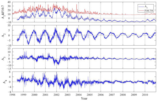
Figure 6.
The distributions of the solar activity index F10.7 and the first four EOF coefficients derived from CODE TEC in China from 1998 to 2010.
It can be seen from Figure 3, Figure 4 and Figure 5 that the spatial and temporal distribution characteristics of the mean value and the first-order EOF base function are relatively consistent, which is consistent with the result in Figure 2 reported by Wan et al. [35]. The spatial distribution mainly reveals the latitude variation features of the ionospheric TEC. The TEC in the Equatorial Ionization Anomaly (EIA) area is the strongest, followed by the near-equatorial area, and the minimum value is in the mid-latitude area [34,36]. The temporal distribution mainly reflects the variation of ionospheric TEC with local time (LT). The amplitude of TEC at 06:00 UT (about 14:00 LT) is significantly larger than that at 00:00 and 12:00 UT. The diurnal variation of ionospheric TEC is mainly controlled by the photochemical processes that change with the Solar Zenith Angle (SZA), showing daily periodic fluctuations. Due to the delay effect of the ionosphere, TEC values typically reach their maximum at around 14:00 LT and minimum near 4:00 LT [38,40].
Figure 6 shows the distributions of the first to fourth-order EOF-decomposed coefficients with DOY from 1998 to 2010. As shown in Figure 6, the amplitude of the coefficient A1 corresponding to the first-order EOF base function demonstrates an evident semi-annual variation, with the maximum amplitude mainly occurring in March and October. At the same time, comparative analysis with the solar activity index F10.7 in Figure 6 shows that the amplitude of the first-order coefficient A1 increases with the increase of solar activity and has an obvious 11-year cycle. The correlation coefficient between the first-order coefficient A1 and the F10.7 index is 0.8880, which is significantly higher than other-order coefficients. The correlation is consistent with the result reported by Mao et al. [33] at Wuhan. The second-order EOF component contains the secondary main variation of TEC, accounting for 3.4580% of the total variation of ionospheric TEC in China. It can be seen from Figure 3, Figure 4 and Figure 5 that the second-order EOF base function is positive in the low latitudes and negative in the middle latitudes. Figure 6 shows that the second-order EOF coefficient A2 has evident annual variation, and its amplitude is smaller than that of the coefficient A1, with the minimum amplitude mainly occurring in March, August, and September. Additionally, the magnitude of A2 is larger in the high solar activity years than in the low solar activity years [32]. The third and fourth-order EOF components account for 1.1965% and 0.7834% of the total variation of ionospheric TEC in China, respectively. It can be seen from Figure 3, Figure 4 and Figure 5 that the third-order EOF base function mainly reflects the redundant information retained after the second-order EOF component is extracted. Since EOF is only a mathematical process, the high-order EOF components still retain some redundant information in the process of decomposition. Accordingly, the spatial distribution characteristics of the third-order EOF base function cannot be well explained physically [29]. Figure 6 clearly shows that the third-order EOF coefficient A3 mainly exhibits the characteristics associated with annual variation, while the fourth-order EOF coefficient A4 mainly shows the characteristics of semi-annual and annual variations, and both are modulated by the solar activity index F10.7. The amplitudes of A3 and A4 are larger in the high solar activity years than in the low solar activity years.
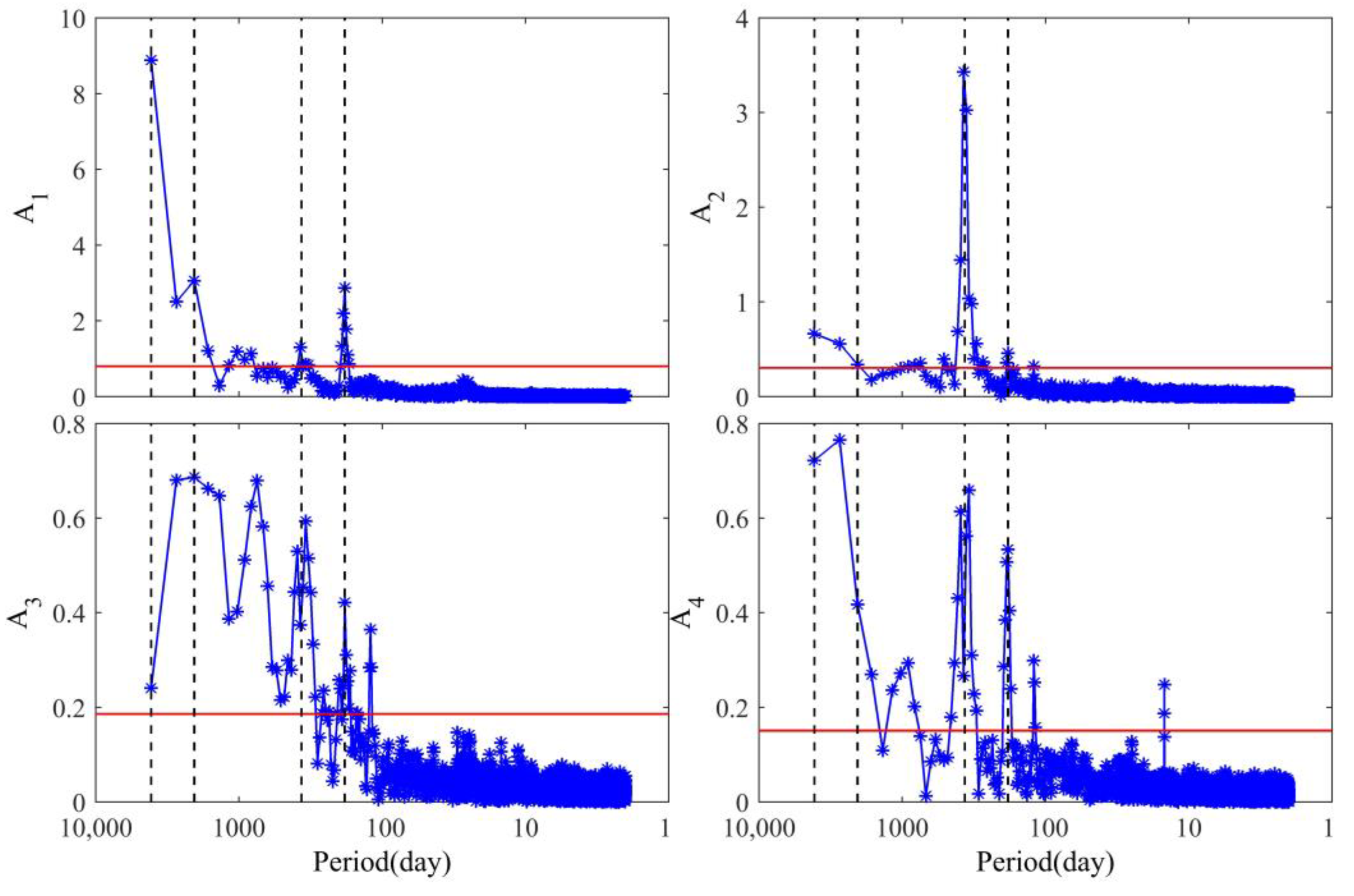
To quantitatively understand the periodic distribution of the first to fourth-order EOF component coefficients, Figure 7 illustrates the periodic spectra of the first to fourth-order EOF component coefficients derived from the fast Fourier transform. In order to show the distribution of the small period more clearly, the logarithm of the X axis is taken in Figure 7. The horizontal red line in Figure 7 represents a confidence level of 95.00%, and the black vertical dotted lines represent 11.21, 5.61, 1.00, and 0.50 years from left to right, respectively. It can be seen from Figure 7 that the first-order coefficient A1 is dominated by 11-year and semi-annual cycles, the second-order coefficient A2 is dominated by annual variation, the third-order coefficient A3 is dominated by 5.61-year and annual cycles, and the fourth-order coefficient A4 is dominated by 11-year, annual, and semi-annual variations. The main cycles observed in each coefficient of different orders are not completely consistent.
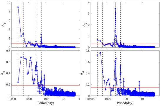
Figure 7.
The period distributions of the first four EOF coefficients derived from CODE TEC in China from 1998 to 2010. The horizontal red line represents the confidence level of 95.00%, and the black vertical dotted lines from left to right represent the period of 11.21, 5.61, 1.00, and 0.50 years, respectively.
3.2. Results of Ionospheric TEC Model over China
The real-time GNSS observation data in China can obtain the vertical TEC at the ionospheric IPP through a certain inversion algorithm, which is referred to as IPP TEC. The IPP TEC shown in the figures are derived by the GNSS data of CMONOC from the first 15 min to the current time. Furthermore, the base functions and coefficients of different orders can be obtained by decomposing CODE TEC in China from 1998 to 2010 through the EOF method. We first select the IPP TEC data of CMONOC from the first 15 min to the current time, and use the historical average value and base function to interpolate the corresponding average values and base function values on the UT, longitude, and latitude of the selected IPP TEC from CMONOC. With the IPP TEC from CMONOC, the interpolated average values, and the interpolated base function values, we use least squares fitting to get the real-time coefficients by Formula (1). Then, the real-time Chinese Ionospheric Map (CIM) can be built by combining the real-time coefficients with the historical base functions and TEC average values, called EOF CIM. EOF CIM can obtain the corresponding TEC at IPP by interpolation, which is called EOF TEC. In order to test the accuracy of the model, the CODE TEC in China is called CODE CIM and is used for comparative analysis with EOF CIM.
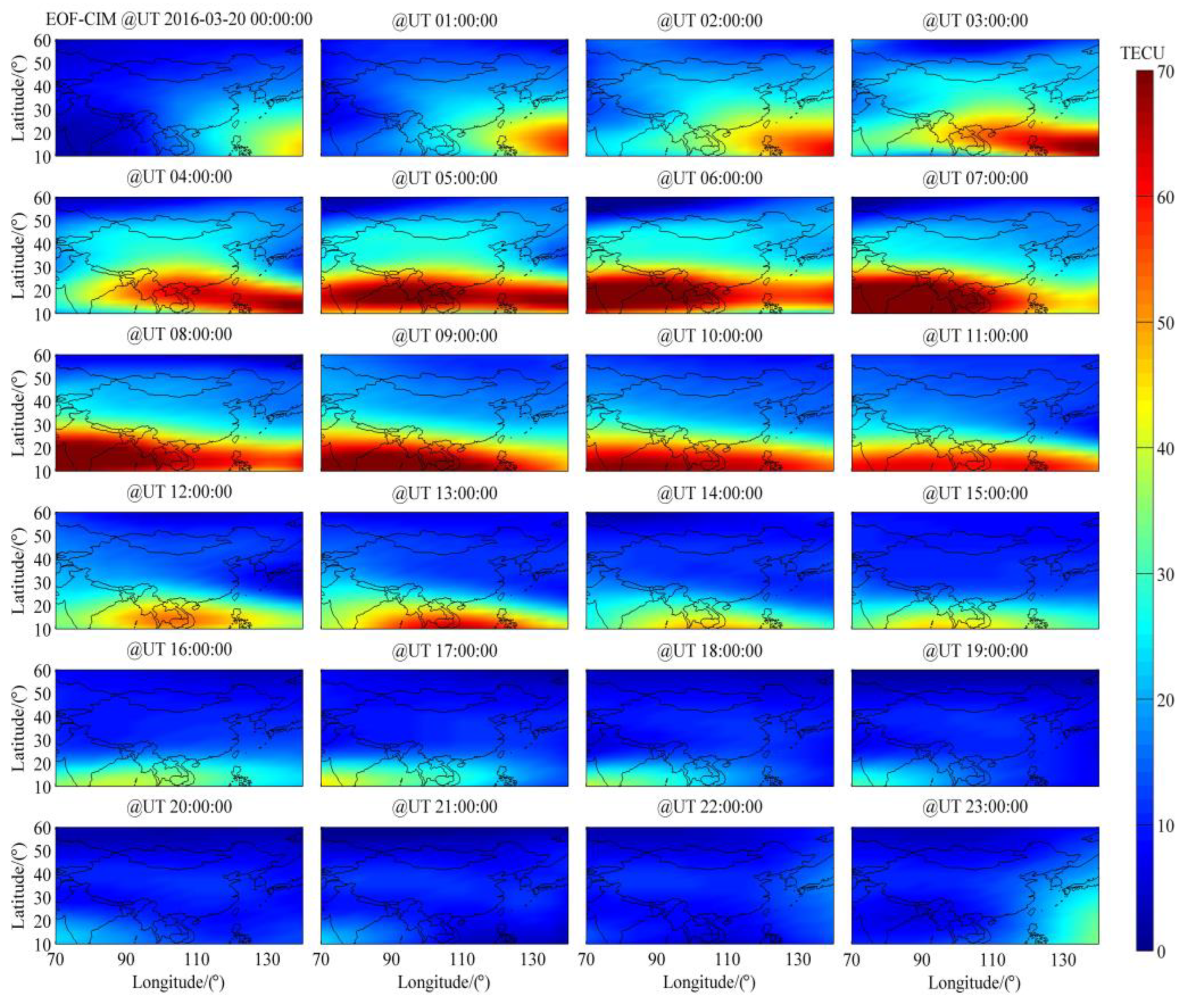
Figure 8 illustrates the distribution of EOF CIM (70°E–140°E, 10°N–60°N) during 00:00–23:00 UT on 20 March 2016. Figure 8 clearly displays the diurnal variation of ionospheric TEC in China that the TEC enhances at sunrise, and which reaches the maximum near 14:00 LT. The latitude range of the EIA area in the spatial distribution can also be clearly shown in Figure 8. Therefore, the regional ionospheric TEC model, which was constructed based on dense GNSS observations combined with the EOF method, can better reflect the temporal and spatial variation characteristics of ionospheric TEC in China [12].
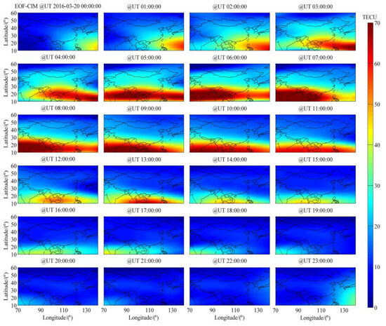
Figure 8.
The distribution of EOF CIM from 00:00 to 23:00 UT on 20 March 2016.
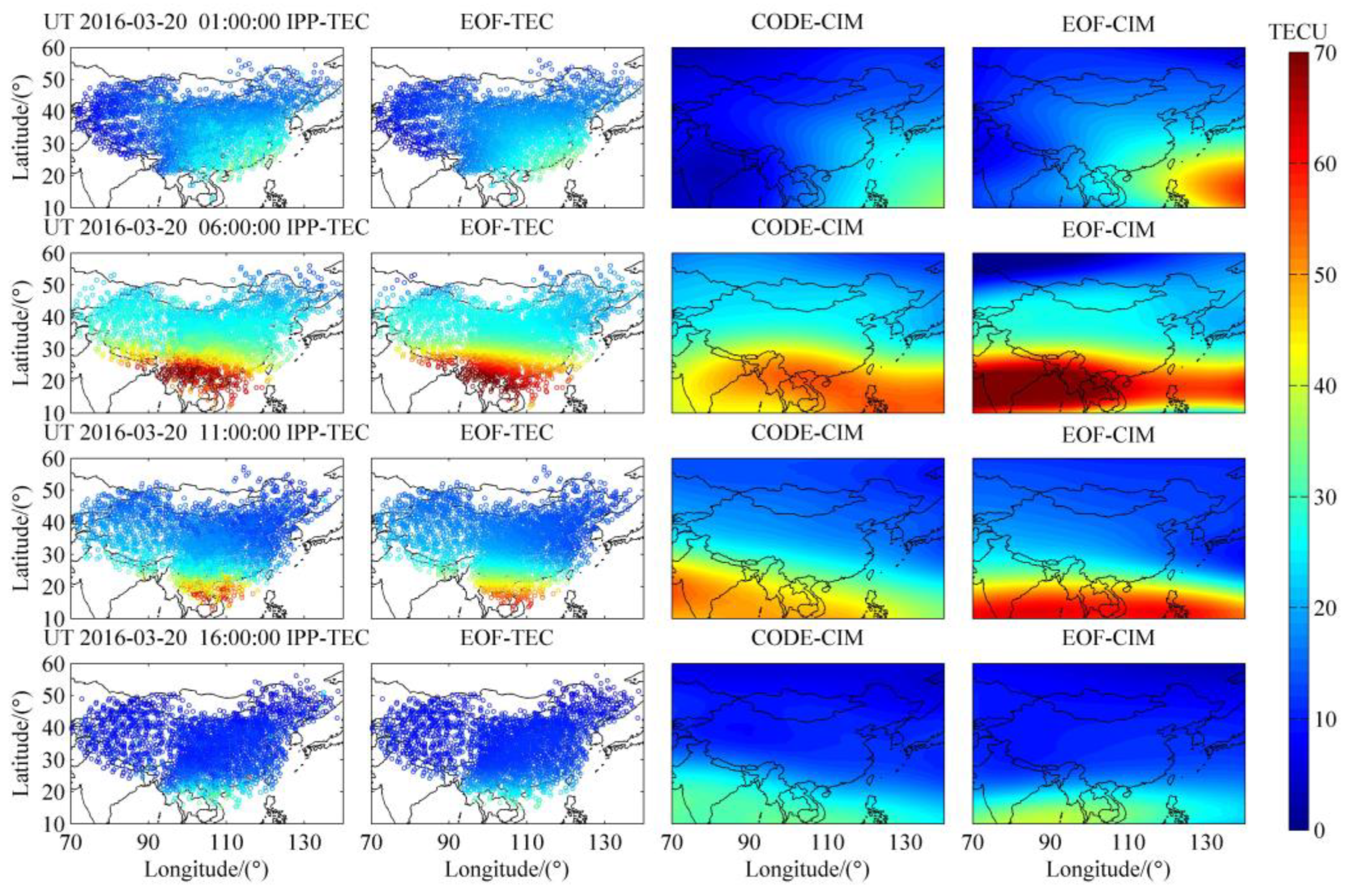
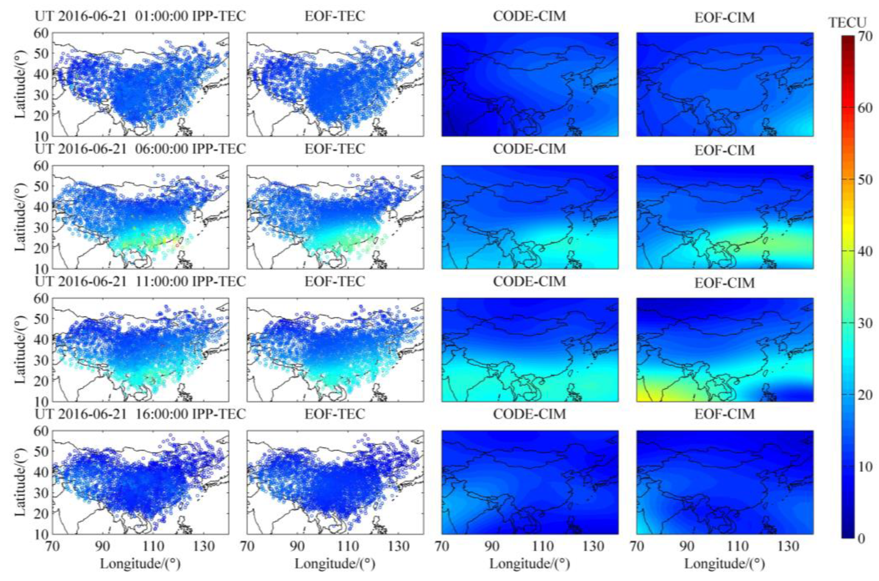
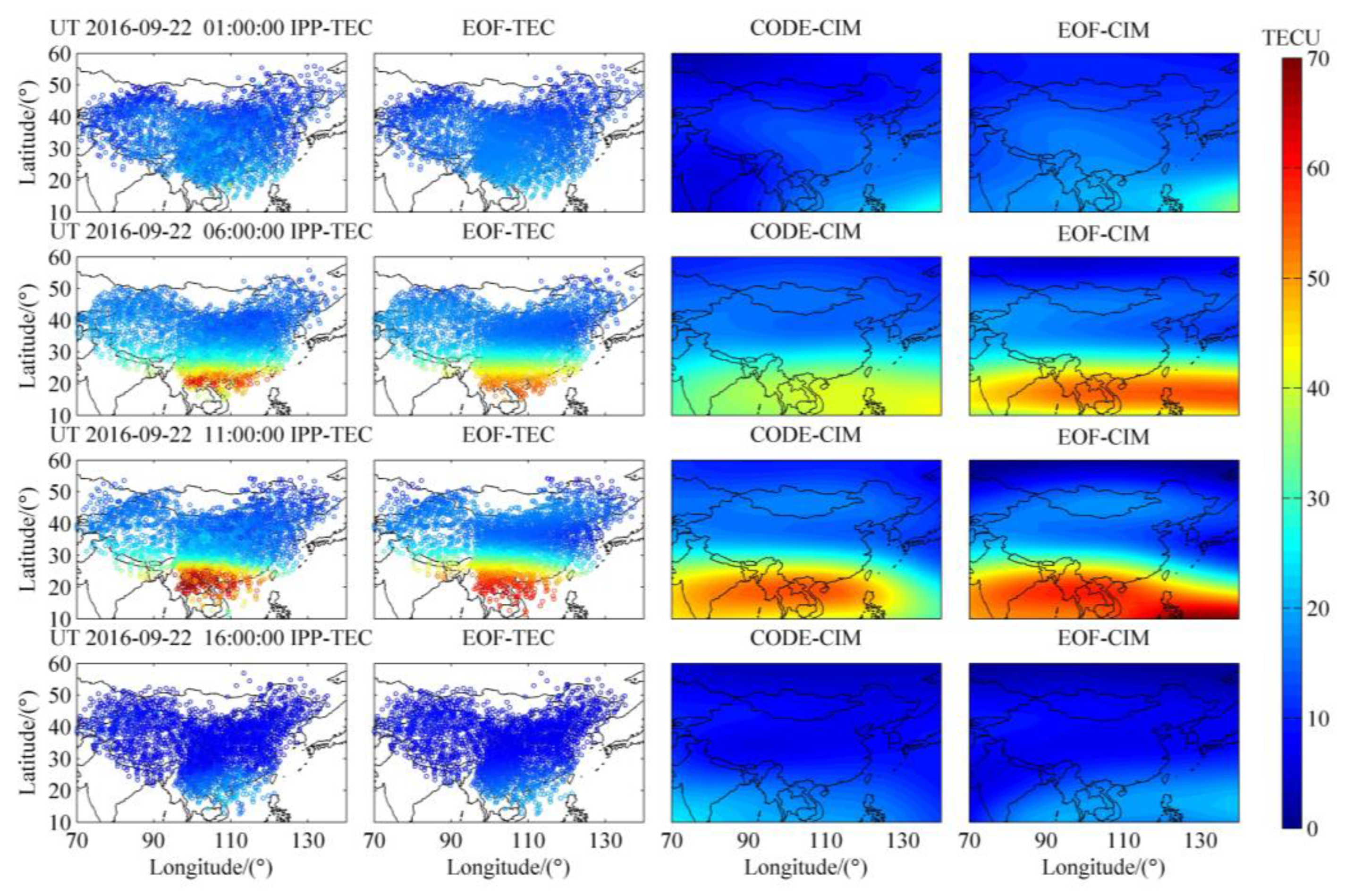
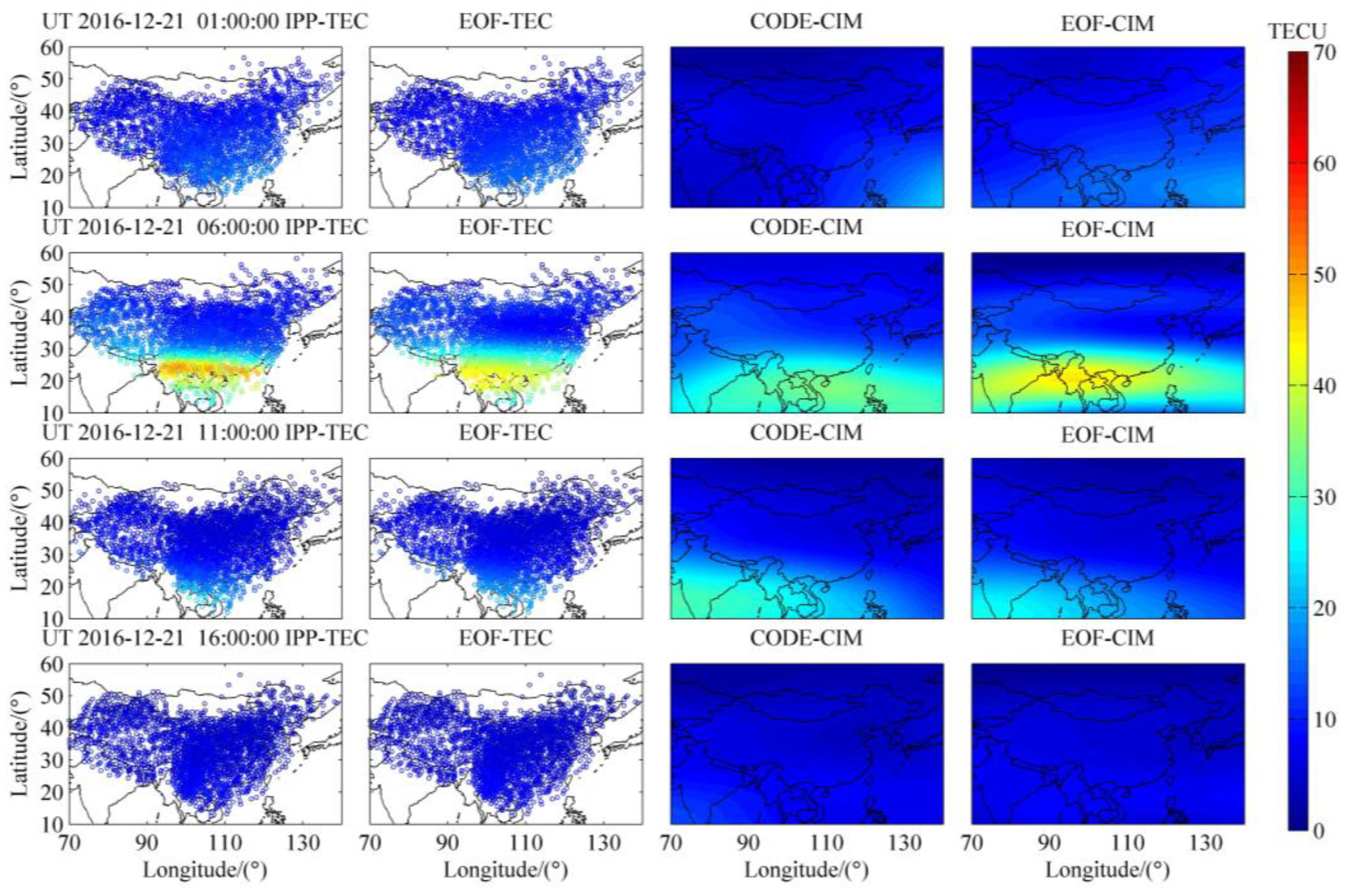
To validate the precision of the constructed Chinese regional ionospheric TEC model (EOF CIM), we compared IPP TEC with EOF TEC, and CODE CIM with EOF CIM in different seasons and UTs. Figure 9, Figure 10, Figure 11 and Figure 12 show the distributions of IPP TEC, EOF TEC, CODE CIM and EOF CIM at 01:00, 06:00, 11:00, and 16:00 UT during the spring equinox, summer solstice, autumn equinox, and winter solstice in 2016. Through the comprehensive comparison of the four figures, it can be seen that the TEC near noon (06:00 UT) is the largest, followed by after sunset (11:00 UT), then after sunrise (01:00 UT), and near midnight (16:00 UT), which is the smallest. In the seasons, the TEC at the spring equinox in 2016 is the largest, followed by the autumn equinox and the winter solstice, and the smallest value of TEC appears in the summer solstice. In the spatial distribution, the latitude and longitude distribution characteristics of IPP TEC, EOF TEC, CODE CIM, and EOF CIM are relatively consistent, especially in the latitude range of the EIA area. However, in the amplitude of TEC in the EIA area, the TEC values of CODE CIM are significantly different from those of IPP TEC, EOF TEC and EOF CIM. The TEC value of CODE CIM in the EIA area near noon (06:00 UT) in Figure 9, Figure 10, Figure 11 and Figure 12 is significantly smaller than those of IPP TEC, EOF TEC and EOF CIM. The difference between CODE CIM and IPP TEC mainly distributes in 0–15 TECU near noon and around 3 TECU in other periods.
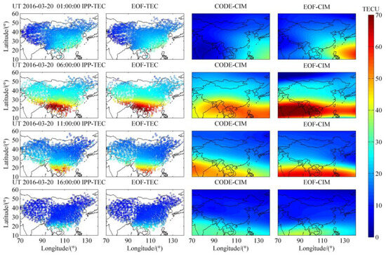
Figure 9.
The distributions of IPP TEC, EOF TEC, CODE CIM, and EOF CIM at 01:00, 06:00, 11:00, and 16:00 UT on 20 March 2016.

Figure 10.
The distributions of IPP TEC, EOF TEC, CODE CIM, and EOF CIM at 01:00, 06:00, 11:00, and 16:00 UT on 21 June 2016.

Figure 11.
The distributions of IPP TEC, EOF TEC, CODE CIM, and EOF CIM at 01:00, 06:00, 11:00, and 16:00 UT on 22 September 2016.
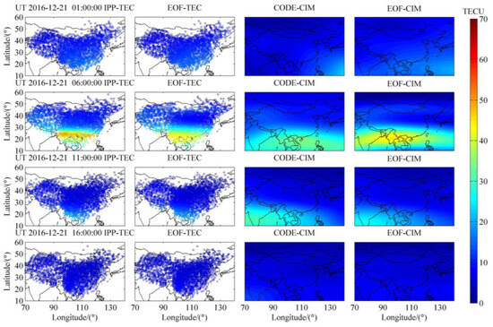
Figure 12.
The distributions of IPP TEC, EOF TEC, CODE CIM, and EOF CIM at 01:00, 06:00, 11:00, and 16:00 UT on 21 December 2016.
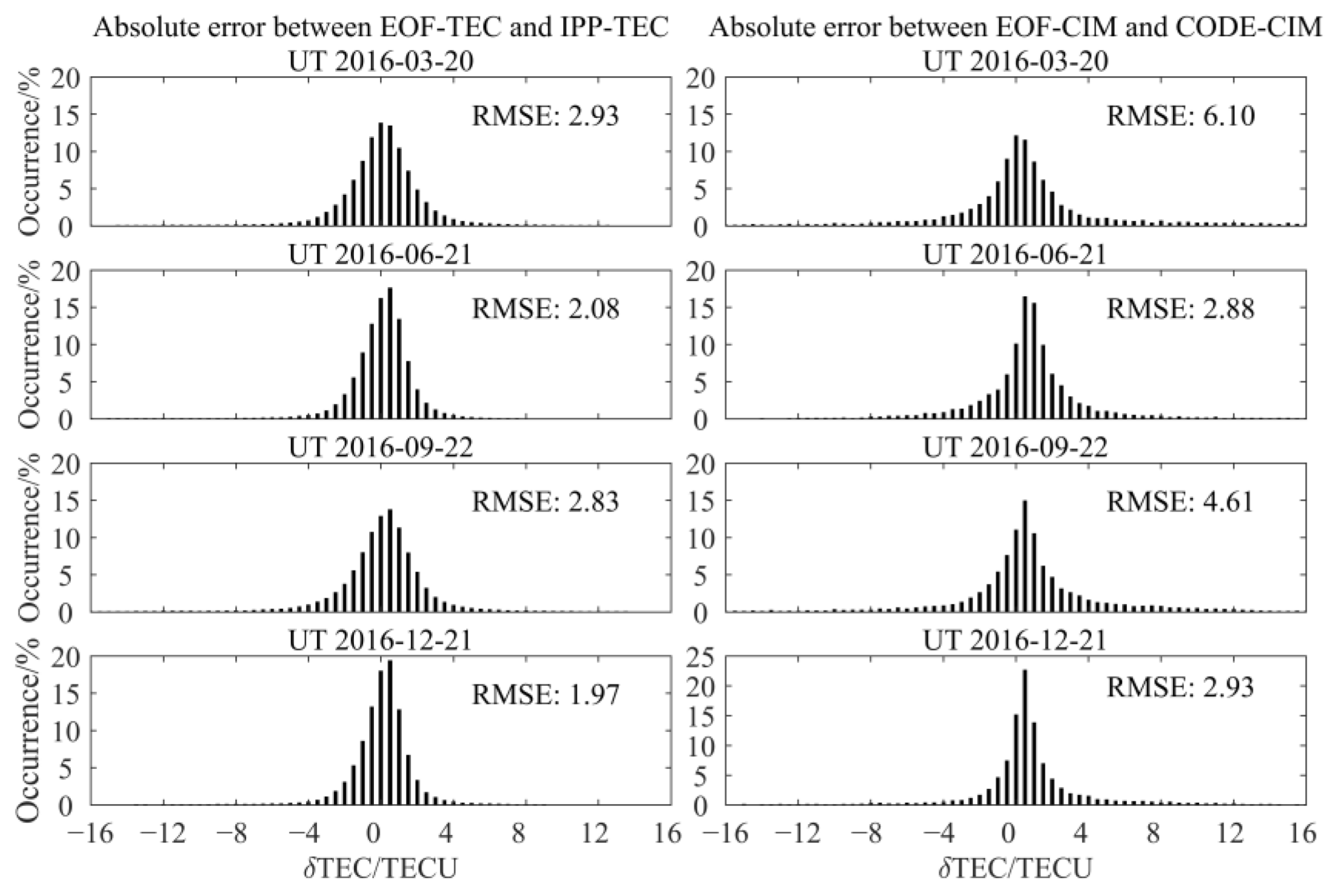
In order to quantitatively analyze the accuracy of the Chinese regional ionospheric TEC model based on dense GNSS observations combined with the EOF method, Figure 13 shows the absolute error distributions between EOF TEC and IPP TEC, EOF CIM and CODE CIM during the spring equinox, summer solstice, autumnal equinox and winter solstice in 2016. It can be seen from Figure 13 that the absolute error between EOF TEC and IPP TEC distributes in −3.50~3.50 TECU, and the root mean square error (RMSE) is around 2.45 TECU. The error analysis shows that EOF CIM is consistent with the actual observations. On the basis of a Kalman filter data assimilation and the GNSS data from CMONOC and International GNSS Service, Aa et al. [12] constructed a regional TEC model over China and adjacent areas. The RMSE between the Madrigal TEC and the TEC obtained from data assimilation has an average amplitude of 2.52 TECU for geomagnetic quiet condition and 3.51 TECU under geomagnetic disturbed condition. The RMSE between EOF TEC and IPP TEC is equivalent to that of the Madrigal TEC and the assimilated TEC in the literature [12]. The absolute error between EOF CIM and CODE CIM distributes in −5.00~5.00 TECU, with RMSE of about 4.49 TECU. The RMSEs in the spring and autumn equinoxes are 6.10 TECU and 4.61 TECU, respectively. A previous study shows that the RMSE between the CODE TEC and the assimilated TEC is around 4.00 TECU under geomagnetic quiet and disturbed conditions [12]. The RMSE between EOF CIM and CODE CIM is slightly larger than between the CODE TEC and the assimilated TEC, reported by Aa et al. [12]. The value of EOF CIM is larger than that of CODE CIM, which is consistent with the distributions of EOF CIM and CODE CIM in the EIA area in Figure 9 and Figure 11. The comprehensive comparative analysis of errors shows that the values of EOF CIM are closer to the observed values in China than those of CODE CIM.
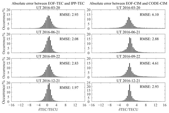
Figure 13.
The absolute error distributions between EOF TEC and IPP TEC, EOF CIM and CODE CIM during the spring equinox, summer solstice, autumn equinox, and winter solstice in 2016.
To further examine the model’s accuracy when the observation data is not involved in the modeling, we first selected the observation data from 4 GNSS stations in the east, south, west, and north directions of China that are not participating in the construction of the EOF CIM. Then, we compared the results obtained from EOF CIM with the observation results of four GNSS stations to analyze the applicability and accuracy of the EOF CIM in different regions of China. The location distribution of the four GNSS stations is shown in the black pentagram in Figure 1, and the relevant station names, along with the geographic latitude and longitude information, are presented in Table 2.
Table 2.
The station names, geographical latitude, and longitude used for model accuracy test and the error distribution for IPP TEC of EOF TEC at each selected station.
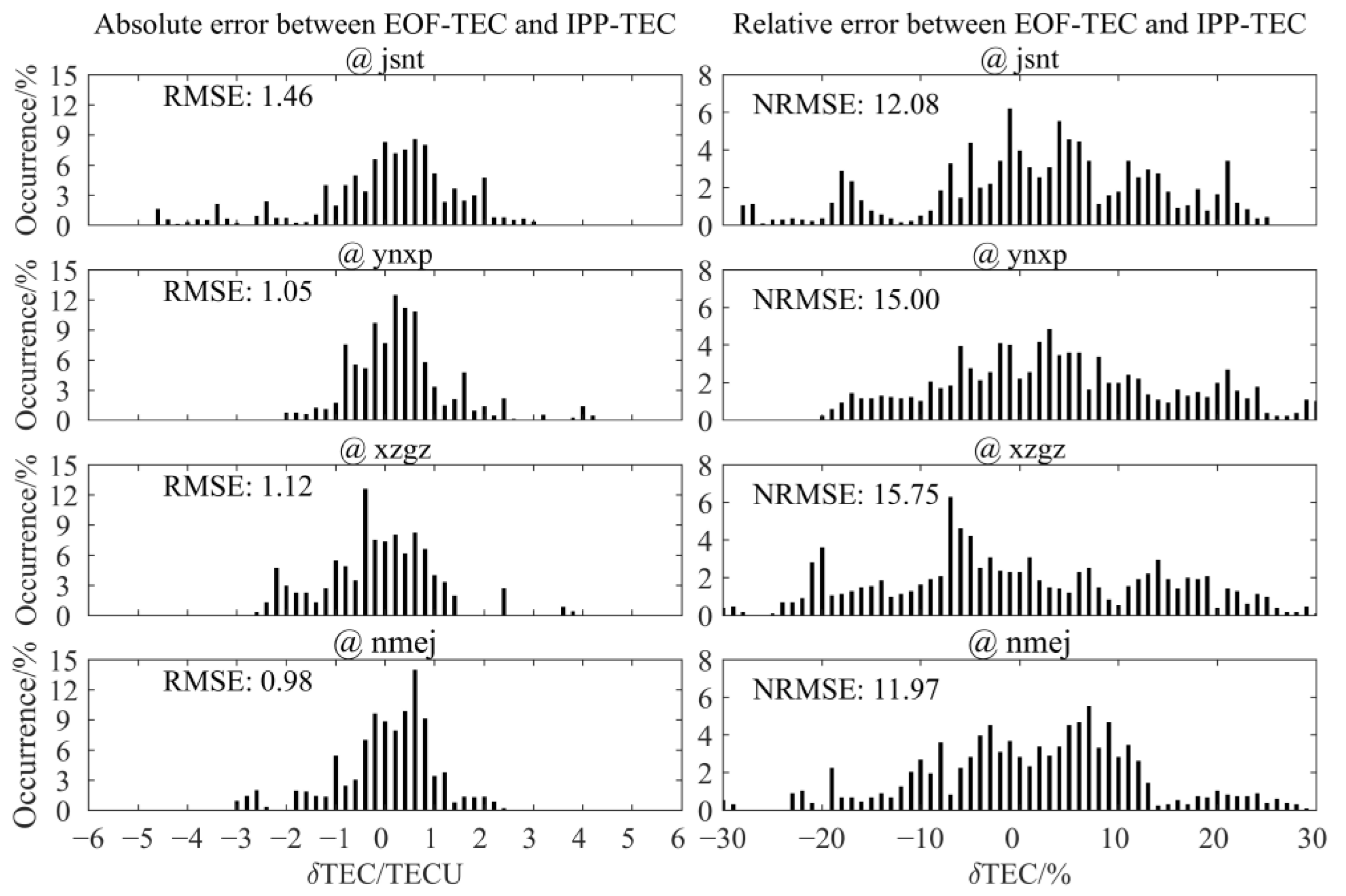
Figure 14 shows the absolute and relative error distributions between IPP TEC of EOF TEC at four GNSS stations (jsnt, ynxp, xzgz, and nmej) in China that are independently not involved in the modeling during the spring equinox, summer solstice, autumnal equinox, and winter solstice in 2016. It can be seen from Figure 14 that the RMSE and the normalized RMSE (NRMSE) [12] between the IPP TEC and EOF TEC for those not involved in the modeling are typically 0.98~1.46 TECU and 11.97~15.75%, respectively. In the west, due to the relatively limited number of observation stations, when the observation data of the western station (xzgz) are not involved in the model construction, the NRMSE is significantly higher compared to the other three stations. Table 2 provides a comparison of error when one of the four GNSS stations is excluded from and included in the modeling process, respectively. Through the comprehensive analysis of Table 2, it can be seen that the accuracy of the model when the observation data of each station are involved in the modeling is higher than that for the non-participant modeling. The model accuracy at the south station (ynxp) shows a significant improvement compared to the other three stations after being included in the modeling.

Figure 14.
The distributions of absolute and relative errors of IPP TEC and EOF TEC at four GNSS stations in China during the spring equinox, summer solstice, autumn equinox, and winter solstice in 2016.
4. Discussion
Figure 6 shows that the amplitude of the coefficient A1 presents an evident semi-annual variation, which is correlated with the geographical longitude. In the same geographical latitude regions, the sectors remote from the magnetic pole are called ‘far-from-polar’ sectors [41]. The semi-annual variation in the ‘far-from-polar’ sectors is affected by the combined effects of the SZA, the high-latitude atmospheric circulation, and the resulting changes in O/N2. In the ‘far-from-polar’ sectors, the geographical latitude where the downwelling air flow appears is relatively high. The SZA in this region approaches 90°, the corresponding generation rate is very small, and it is very sensitive to the SZA. Even if the downwelling produces a large O/N2, it still cannot produce substantial electrons [29,42]. Therefore, in China, which belongs to the ‘far-from-polar’ sectors, the production rate is very small in the winter and increases with the increase of the zenith angle in the spring equinox. The O/N2 decreases in the summer, which leads to two peaks of TEC in March and October, resulting in the semi-annual variation of coefficient A1. In addition, the analysis of the ionospheric theoretical model [43] shows that the semi-annual variation of the low-latitude electric field strengthens the semi-annual variation of the ionospheric parameters in the EIA region [44]. In addition, some studies show that the semi-annual variation of the diurnal tide in the thermosphere can strengthen the semi-annual variation of the equatorial electrojet, which enhances the semi-annual variation of the ionosphere in the low latitudes through the dynamic effect [29,45].
Figure 9, Figure 10, Figure 11 and Figure 12 show that the asymmetry of the ionospheric TEC between spring and autumn equinoxes is more noticeable in the low-latitude region [46,47]. Liu et al. [48] indicated that the ionospheric TEC in the low-latitude region at 14:00 LT of low solar activity is weaker in September than in March. Their result is consistent with the distribution of the TEC in the low-latitude region near noon (06:00 UT) in the spring and autumn equinoxes of 2016, as shown in Figure 9 and Figure 11, which is mainly due to the fact that the phase of the annual variation component of the TEC is located in January, and the amplitude is larger at low latitudes. Figure 9 and Figure 11 show that the TEC after sunset (11:00 UT) of the autumn equinox exceeds that near the midday of the autumn equinox or after sunset of the spring equinox, which is obviously different from the asymmetric distribution of the ionospheric TEC at 18:00 LT in the spring and autumn equinoxes under low solar activity, as shown in Figure 9 of Liu et al. [48].
5. Conclusions
In this study, the EOF method is first applied to analyze the CODE TEC in China from 1998 to 2010. Then, the real-time coefficients of the EOF components are fitted by the real-time intensive GNSS observation data of CMONOC. Subsequently, the real-time ionospheric TEC model EOF CIM in China is constructed by combining the real-time coefficients, base functions, and the historical TEC average value. Finally, the results of EOF CIM are compared with IPP TEC and CODE CIM. The specific findings are summarized as follows:
(1) The spatial and temporal distribution characteristics of the average value of CODE TEC in China from 1998 to 2010 are consistent with that of the first-order base function after EOF decomposition, which mainly reflects the latitude and diurnal variation characteristics of TEC in China. The second-order EOF base function is positive in the low latitudes and negative in the middle latitudes. The first four EOF components account for 90.3813%, 3.4580%, 1.1965%, and 0.7834% of the total variation of ionospheric TEC in China, respectively.
(2) The amplitude of the first-order EOF coefficient A1 demonstrates an evident semi-annual variation, and the maximum amplitude mainly appears in March and October. This is mainly attributed to the change of geographical longitude, the semi-annual variation of the low-latitude electric field, and the ionospheric fountain effect. Additionally, A1 also has a clear cycle of about 11 years, and the correlation coefficient with the F10.7 index is 0.8880. The amplitude of the second-order EOF coefficient A2 has an obvious annual variation, and its amplitude is smaller than the amplitude of the coefficient A1. The minimum value of the amplitude mainly occurs in March, August, and September. At the same time, the amplitude of A2 in high solar activity years is larger than that in low solar activity years. The third-order EOF coefficient A3 mainly shows the characteristics of annual variation, while the fourth-order EOF coefficient A4 mainly shows the characteristics of annual and semi-annual variations, and A3 and A4 are both modulated by the solar activity index F10.7. The period spectrum analysis of the fast Fourier transform shows that the periods of 11.21, 5.61, 1.00, and 0.50 years are evident in the first to fourth-order EOF coefficients.
(3) The ionospheric TEC model EOF CIM, driven by the real-time GNSS observation data of CMONOC, can well reflect the latitude, LT, and seasonal variation characteristics of ionospheric TEC in China. The model results show that the TEC after sunset of the autumn equinox exceeds that near the midday of the autumn equinox, or after sunset of the spring equinox. This is obviously different from the asymmetric distribution of the ionospheric TEC at 18:00 LT in the spring and autumn equinoxes under low solar activity in previous reports. The model’s comparative analysis and error test show that the RMSE between EOF TEC and IPP TEC is mainly distributed around 2.45 TECU, and the RMSE between EOF CIM and CODE CIM is typically around 4.49 TECU. A previous study indicates that the RMSE between the assimilated TEC and the Madrigal TEC is 2.52 TECU under geomagnetic quiet conditions, and the RMSE between the assimilated TEC and the CODE TEC is around 4.00 TECU under geomagnetic quiet and disturbed conditions. The results of the EOF CIM model are closer to the actual observation in China than those of the CODE CIM model. Furthermore, the comparative analysis results show that the increase of GNSS observation data involved in modeling is advantageous for improving the accuracy of the ionospheric TEC model in China.
The above research shows that the Chinese ionospheric TEC model EOF CIM, constructed by the EOF method combined with dense real-time GNSS observation data, can quickly give the real-time distribution of ionospheric TEC in China. The spatial and temporal distributions of EOF CIM are consistent with the distributions of the observed IPP TEC. The high-accuracy ionospheric TEC model can provide important technical support for the study of ionospheric regional characteristics in China and the correction of satellite navigation radio waves.
Author Contributions
Conceptualization, B.X.; Methodology, B.X., B.Z. and F.D.; Formal analysis, Y.L. and X.L.; Validation, Y.L., C.Y., Y.W. and L.D.; Data curation, J.L. and L.H.; Writing—original draft preparation, B.X. and Y.L.; Writing—review and editing, B.X., Y.L., B.Z. and L.H. All authors have read and agreed to the published version of the manuscript.
Funding
This work was supported by the Natural Science Foundation of Hebei Province (Grant No. D2022502001 and D2019502010), Fundamental Research Funds for the Central Universities (2018MS128), the National Natural Science Foundation of China (41574151, 41574162, and 41404127), and the National High Technology Research and Development Program of China (2014AA123503).
Data Availability Statement
The data presented in this study are available from the corresponding author upon reasonable request.
Acknowledgments
Thanks to the Center for Orbit Determination in Europe for providing the global ionosphere maps and the Crustal Movement Observation Network of China for providing the GNSS data in this study.
Conflicts of Interest
The authors declare no conflict of interest.
References
- Liu, L.; Yang, Y.; Le, H.; Chen, Y.; Zhang, R.; Zhang, H.; Sun, W.; Li, G. Unexpected Regional Zonal Structures in Low Latitude Ionosphere Call for a High Longitudinal Resolution of the Global Ionospheric Maps. Remote Sens. 2022, 14, 2315. [Google Scholar] [CrossRef]
- Hernández-Pajares, M.; Juan, J.M.; Sanz, J.; Orus, R.; Garcia-Rigo, A.; Feltens, J.; Komjathy, A.; Schaer, S.C.; Krankowski, A. The IGS VTEC maps: A reliable source of ionospheric information since 1998. J. Geod. 2009, 83, 263–275. [Google Scholar] [CrossRef]
- Xiong, B.; Wan, W.; Zhao, B.; Yu, Y.; Wei, Y.; Ren, Z.; Liu, J. Response of the American equatorial and low-latitude ionosphere to the X1. 5 solar flare on 13 September 2005. J. Geophys. Res. Space Phys. 2014, 119, 10336–10347. [Google Scholar] [CrossRef]
- Huo, X.L.; Yuan, Y.B.; Ou, J.K.; Zhang, K.F.; Bailey, G.J. Monitoring the global-scale winter anomaly of total electron contents using GPS data. Earth Planets Space 2009, 61, 1019–1024. [Google Scholar] [CrossRef]
- Xiong, B.; Wan, W.; Ning, B.; Ding, F.; Hu, L.; Yu, Y. A statistic study of ionospheric solar flare activity indicator. Space Weather 2014, 12, 29–40. [Google Scholar] [CrossRef]
- Jin, S.; Wang, Q.; Dardanelli, G. A Review on Multi-GNSS for Earth Observation and Emerging Applications. Remote Sens. 2022, 14, 3930. [Google Scholar] [CrossRef]
- De Franceschi, G.; De Santis, A.; Pau, S. Ionospheric mapping by regional spherical harmonic analysis: New developments. Adv. Space Res. 1994, 14, 61–64. [Google Scholar] [CrossRef]
- Lanyi, G.E.; Roth, T. A comparison of mapped and measured total ionospheric electron content using global positioning system and beacon satellite observations. Radio Sci. 1988, 23, 483–492. [Google Scholar] [CrossRef]
- Ping, J.; Kono, Y.; Matsumoto, K.; Otsuka, Y.; Saito, A.; Shum, C.; Heki, K.; Kawano, N. Regional ionosphere map over Japanese Islands. Earth Planets Space 2002, 54, e13–e16. [Google Scholar] [CrossRef]
- Yuan, Y.; Ou, J. A generalized trigonometric series function model for determining ionospheric delay. Prog. Nat. Sci. 2004, 14, 1010–1014. [Google Scholar] [CrossRef]
- Opperman, B.D.L.; Cilliers, P.J.; McKinnell, L.A.; Haggard, R. Development of a regional GPS-based ionospheric TEC model for South Africa. Adv. Space Res. 2007, 39, 808–815. [Google Scholar] [CrossRef]
- Aa, E.; Huang, W.G.; Yu, S.M.; Liu, S.Q.; Shi, L.Q.; Gong, J.C.; Chen, Y.H.; Shen, H. A regional ionospheric TEC mapping technique over China and adjacent areas on the basis of data assimilation. J. Geophys. Res. Space Phys. 2015, 120, 5049–5061. [Google Scholar] [CrossRef]
- Li, Z.S.; Wang, N.B.; Li, M.; Zhou, K.; Yuan, Y.B.; Hong, Y. Evaluation and analysis of the global ionospheric TEC map in the frame of international GNSS services. Chin. J. Geophys. 2017, 60, 3718–3729. [Google Scholar]
- Wen, D.; Tang, Y.; Xie, K. A Novel Method of Ionospheric Inversion Based on Horizontal Constraint and Empirical Orthogonal Function. Remote Sens. 2023, 15, 3124. [Google Scholar] [CrossRef]
- Bust, G.S.; Garner, T.W.; Gaussiran, T.L. Ionospheric Data Assimilation Three-Dimensional (IDA3D): A global, multisensor, electron density specification algorithm. J. Geophys. Res. Space Phys. 2004, 109, A11312. [Google Scholar] [CrossRef]
- Xu, W.Y.; Kamide, Y. Decomposition of daily geomagnetic variations by using method of natural orthogonal co mponent. J. Geophys. Res. Space Phys. 2004, 109, A05218. [Google Scholar] [CrossRef]
- Zhao, B.; Wan, W.X.; Liu, L.B.; Chen, Y.D.; Le, H.J. Statistical characteristics of the total ion density in the topside ionosphere during the period 1996-2004 using empirical orthogonal function (EOF). Ann. Geophys. 2005, 23, 3615–3631. [Google Scholar] [CrossRef]
- Liu, C.X.; Zhang, M.L.; Wan, W.X.; Liu, L.B.; Ning, B.Q. Modeling M (3000) F2 based on empirical orthogonal function analysis method. Radio Sci. 2008, 43, RS1003. [Google Scholar] [CrossRef]
- Zhang, M.L.; Liu, C.X.; Wan, W.X.; Liu, L.B.; Ning, B.Q. Evaluation of global modeling of M (3000) F2 and hmF2 based on alternative empirical orthogonal function expansions. Adv. Space Res. 2010, 46, 1024–1031. [Google Scholar] [CrossRef]
- Uwamahoro, J.C.; Habarulema, J.B. Modelling total electron content during geomagnetic storm conditions using empirical orthogonal functions and neural networks. J. Geophys. Res. Space Phys. 2015, 120, 11000–11012. [Google Scholar] [CrossRef]
- Talaat, E.R.; Zhu, X. Spatial and temporal variation of total electron content as revealed by principal component analysis. Ann. Geophys. 2016, 34, 1109–1117. [Google Scholar] [CrossRef]
- Dabbakuti, J.R.K.K.; Ratnam, D.V. Characterization of ionospheric variability in TEC using EOF and wavelets over low-latitude GNSS stations. Adv. Space Res. 2016, 57, 2427–2443. [Google Scholar] [CrossRef]
- Dabbakuti, J.R.K.K.; Ratnam, D.V. Modeling and analysis of GPS-TEC low latitude climatology during the 24th solar cycle using empirical orthogonal functions. Adv. Space Res. 2017, 60, 1751–1764. [Google Scholar] [CrossRef]
- She, C.L.; Wan, W.X.; Yue, X.N.; Xiong, B.; Yu, Y.; Ding, F.; Zhao, B.Q. Global ionospheric electron density estimation based on multisource TEC data assimilation. GPS Solut. 2017, 21, 1125–1137. [Google Scholar] [CrossRef]
- Andima, G.; Amabayo, E.B.; Jurua, E.; Cilliers, P.J. Modeling of GPS total electron content over the African low-latitude region using empirical orthogonal functions. Ann. Geophys. 2019, 37, 65–76. [Google Scholar] [CrossRef]
- Chen, P.; Liu, H.; Ma, Y. Empirical orthogonal function analysis and modeling of global ionospheric spherical harmonic coefficients. GPS Solut. 2020, 24, 1–17. [Google Scholar] [CrossRef]
- Owolabi, C.; Ruan, H.B.; Yamazaki, Y.; Li, J.F.; Zhong, J.H.; Eyelade, A.V.; Priyadarshi, S.; Yoshikawa, A. Empirical modeling of ionospheric current using empirical orthogonal function analysis and artificial neural network. Space Weather 2021, 19, e2021SW002831. [Google Scholar] [CrossRef]
- Zhang, S.R.; Chen, Z.W.; Coster, A.J.; Erickson, P.J.; Foster, J.C. Ionospheric symmetry caused by geomagnetic declination over North America. Geophys. Res. Lett. 2013, 40, 5350–5354. [Google Scholar] [CrossRef]
- Yao, X.; Zhao, B.Q.; Liu, L.B.; Wan, W.X. Comparison of ionospheric total electron content over North America and East Asia with EOF analysis. Chin. J. Space Sci. 2015, 35, 556–565. [Google Scholar] [CrossRef]
- Chen, Z.W.; Zhang, S.R.; Coster, A.J.; Fang, G.Y. EOF analysis and modeling of GPS TEC climatology over North America. J. Geophys. Res. Space Phys. 2015, 120, 3118–3129. [Google Scholar] [CrossRef]
- A, E.; Zhang, D.H.; Xiao, Z.; Hao, Y.Q.; Ridley, A.J.; Moldwin, M. Modeling ionospheric foF2 by using empirical orthogonal function analysis. Ann. Geophys. 2011, 29, 1501–1515. [Google Scholar]
- Yu, Y.; Wan, W.X.; Xiong, B.; Ren, Z.P.; Zhao, B.Q.; Zhang, Y.; Ning, B.Q.; Liu, L.B. Modeling Chinese ionospheric layer parameters based on EOF analysis. Space Weather 2015, 13, 339–355. [Google Scholar] [CrossRef]
- Mao, T.; Wan, W.X.; Liu, L.B. An EOF-based empirical model of TEC over Wuhan. Chin. J. Geophys. 2005, 48, 751–758. [Google Scholar] [CrossRef]
- Mao, T.; Wan, W.X.; Yue, X.N.; Sun, L.F.; Zhao, B.Q.; Guo, J.P. An empirical orthogonal function model of total electron content over China. Radio Sci. 2008, 43, RS2009. [Google Scholar] [CrossRef]
- Wan, W.X.; Ding, F.; Ren, Z.P.; Zhang, M.L.; Liu, L.B.; Ning, B.Q. Modeling the global ionospheric total electron content with empirical orthogonal function analysis. Sci. China Technol. Sci. 2012, 55, 1161–1168. [Google Scholar] [CrossRef]
- Li, S.H.; Zhou, H.X.; Xu, J.J.; Wang, Z.Q.; Li, L.H.; Zheng, Y.L. Modeling and analysis of ionosphere TEC over China and adjacent areas based on EOF method. Adv. Space Res. 2019, 64, 400–414. [Google Scholar] [CrossRef]
- Xiong, B.; Li, X.L.; Wan, W.X.; She, C.L.; Hu, L.H.; Ding, F.; Zhao, B.Q. A method for estimating GNSS instrumental biases and its application based on a receiver of multisystem. Chin. J. Geophys. 2019, 62, 1199–1209. [Google Scholar]
- Xiong, B.; Wan, W.X.; Yu, Y.; Hu, L.H. Investigation of ionospheric TEC over China based on GNSS data. Adv. Space Res. 2016, 58, 867–877. [Google Scholar] [CrossRef]
- Li, Q.; Ning, B.Q.; Zhao, B.Q.; Ding, F.; Zhang, R.; Shi, H.B.; Yue, H.J.; Li, G.Z.; Li, J.Y.; Han, Y.F. Applications of the CMONOC based GNSS data in monitoring and investigation of ionospheric space weather. Chin. J. Geophys. 2012, 55, 2193–2202. [Google Scholar]
- Xiong, B.; Wan, W.X.; Ning, B.Q.; Hu, L.H.; Ding, F.; Zhao, B.Q.; Li, J.Y. Investigation of mid- and low-latitude ionosphere based on BDS, GLONASS and GPS observations. Chin. J. Geophys. 2014, 57, 3586–3599. [Google Scholar]
- Rishbeth, H. How the thermospheric circulation affects the ionospheric F2-layer. J. Atmos. Sol. -Terr. Phys. 1998, 60, 1385–1402. [Google Scholar]
- Rishbeth, H.; Muller-Wodarg, I.C.F.; Zou, L.; Fuller-Rowell, T.J.; Millward, G.H.; Moffett, R.J.; Idenden, D.W.; Aylward, A.D. Annual and semiannual variations in the ionospheric F2-layer: II. Physical discussion. Ann. Geophys. 2000, 18, 945–956. [Google Scholar]
- Yu, T.; Wan, W.X.; Liu, L.B. A theoretical model for ionospheric electric fields at mid-and low-latitudes. Sci. China Ser. G 2003, 46, 23–32. [Google Scholar]
- Yu, T.; Wan, W.X.; Liu, L.B.; Li, X.Y.; Luan, X.L.; Tang, W. A simulation study on the semiannual variation of the ionospheric F2 layer zonal electric fields at the magnetic equator. J. Geophys. Res. Space Phys. 2006, 111, A09310. [Google Scholar]
- Ma, R.; Xu, J.; Liao, H. The features and a possible mechanism of semiannual variation in the peak electron density of the low latitude F2 layer. J. Atmos. Sol. -Terr. Phys. 2003, 65, 47–57. [Google Scholar]
- Liu, L.B.; He, M.S.; Yue, X.A.; Ning, B.Q.; Wan, W.X. Ionosphere around equinoxes during low solar activity. J. Geophys. Res. Space Phys. 2010, 115, A09307. [Google Scholar]
- Chen, Y.D.; Liu, L.B.; Wan, W.X.; Yue, X.A.; Su, S.Y. Solar activity dependence of the topside ionosphere at low latitudes. J. Geophys. Res. Space Phys. 2009, 114, A08306. [Google Scholar]
- Liu, Y.; Chen, Y.D.; Liu, L.B. Local time dependence of ionospheric equinoctial asymmetry. Chin. J. Geophys. 2016, 59, 3941–3954. [Google Scholar]


Disclaimer/Publisher’s Note: The statements, opinions and data contained in all publications are solely those of the individual author(s) and contributor(s) and not of MDPI and/or the editor(s). MDPI and/or the editor(s) disclaim responsibility for any injury to people or property resulting from any ideas, methods, instructions or products referred to in the content. |
© 2023 by the authors. Licensee MDPI, Basel, Switzerland. This article is an open access article distributed under the terms and conditions of the Creative Commons Attribution (CC BY) license (https://creativecommons.org/licenses/by/4.0/).