Feature Importance Ranking of Random Forest-Based End-to-End Learning Algorithm

Abstract

Efficient land management and farming practices are critical to maintaining agricultural production, especially in Europe with limited arable land. It is very time consuming to rely on a manual field inspection of cultivated land to archive farm crops. But with the help of satellite monitoring data on the earth’s surface, it is a new vision to classify farmland based on deep learning. This article has studied the Sentinel 2 (S2) data, which are top-of-atmosphere (TOA) reflectance values at the processing level-1C (L1C) observed from some areas of Germany and France. Aiming at the problem that the interference of atmosphere and cloud coverage weakens the recognition accuracy of subsequent algorithms, a method of combining feature expansion and feature importance analysis is proposed to optimize the raw S2 data. Specifically, the new 13 spectral features are expanded based on the linear and nonlinear combination of the raw 13 spectral bands of S2. The random forest (RF) algorithm is used to score the importance of features, and the important features of each time series are selected to form a new dataset. Then, an end-to-end deep learning model has been used for training. The structure of the model is a two-layer unidirectional recurrent neural network with long short-term memory (LSTM) as the backbone. And two linear layers as the output, which form two decision-making heads, respectively, representing output classification probability and the stop decision. The results show that adding features and selecting features is beneficial for the model to improve classification accuracy and predict the classification without all of the input data. This end-to-end classification pattern with early prediction would support intelligent monitoring of farm crops with a great advantage to the implementation of various agricultural policies.

1. Introduction

The implementation of the Landsat program [1], the Copernicus program [2], and the Gaofen project [3] have enabled satellites to monitor the earth with higher-resolution data, and the fields where the data play a role have been further expanded [4,5,6]. In terms of the Copernicus program, there exist six tasks consisting of Sentinel missions, which provide us with the vast majority of data in applications ranging from land and ocean observation crop monitoring, climate monitoring, and atmospheric monitoring [2]. Especially, Sentinel 2 (S2) allows additional channels in the red edge spectral domain to assess the vegetation status. However, the free data seem not been fully exploited from the downloads of remote sensing (RS) data on the Google Earth Engine (GEE) platform launched by Google.

Mainly, the one challenge is that the raw data mixed up with the atmosphere and cloud reflectivity make it much more difficult to extract effective information to achieve goals like crop classification. Therefore, from the previous literature on agricultural RS, researchers have dedicated themselves to studying vegetation indexes (VIs) to improve data quality and availability [7,8,9,10,11]. To a certain extent, phenological characterization makes sense to classify land cover types based on multitemporal seasonal spectral responses. The normalized difference vegetation index (NDVI) [12] has been proven the best indicator of vegetation growth status and vegetation coverage. The enhanced vegetation index (EVI) [12], the inheritance and improvement of the NDVI, introduced an atmosphere-sensitive blue band to correct the red band for aerosol influences which has higher sensitivity and superiority in monitoring vegetation changes.

VIs reflect the response characteristics of vegetation to different spectral bands. For different types of crops, the VI time series show different characteristics due to their differences in phenological characteristics. Therefore, they are an important research object in agricultural RS monitoring.

For example, Zhang et al. [7] identified winter wheat by integrating spectral and temporal information derived from multi-resolution RS data and specifically proposed a new method to express the quantitative relationship between MODIS NDVI time series data and actual crop planting area. the main crops of Uzbekistan wheat, rice, and cotton were classified through phenology, tasseled cap, and rule-based classification using high-resolution (15–30 m) bi-temporal data [13]. The applicability of time-series MODIS 250 m VI data concluded that the NDVI with date-of-acquisition interpolation emerged as the optimal dataset is the best for crop classification in Mato Grosso, Brazil [11]. However, Damien Arvor [8] found that on a regional scale, MODIS EVI time series data can effectively detect the spatiotemporal dynamics of agricultural regions. In addition, a classification method that used phenological indices calculated from the EVI time series as an input avoids the restrictive requirements of large ground reference datasets. So, it enables frequent and routine crop mapping without the repeated collection of reference data [14]. Moreover, when developing accurate crop distribution maps, a method called object-based crop identification and mapping is proposed, which combines 12 VIs to evaluate a large number of crop types and field conditions. However, it needs future analysis to evaluate its robustness [10]. Furthermore, three VIs were added to the S2 band. Different variable combinations were tested to obtain reliable data collection to improve subsequent classification steps by exploiting the full potential of GEE [9].The aforementioned focuses on several VIs to prove their ability to delineate the characteristics of surface objects.

Additionally, another challenge is how to fit the big RS data. Fortunately, deep learning (DL) networks are a good avenue for time series classification and prediction, which can handle large-scale data. Pelletier et al. [15] carrued iyt comprehensive research on temporal convolutional neural networks (TempCNNs), quantitatively and qualitatively evaluated the contribution of TempCNNs to satellite image time series classification, and proposed that pooling layers should be carefully studied before integrating into TempCNN networks. However, they advised against adding manually calculated spectral features such as the NDVI as it doesn’t seem to improve the TempCNN model. To solve the problems of accuracy and time complexity, Fawaz et al. [16] inspired by the Inception-v4 architecture, proposed a collection of deep convolutional neural network (CNN) models. This is a collection of CNN models inspired by the Inception-v4 architecture that can learn from 1500 time series in 1 h and 13 M time series in 8 h. For processing from satellite sequences, Kussul et al. [17] proposed a multi-layer DL architecture that aims for pixel-level classification of source multitemporal RS images, including optical and SAR. At the heart of the architecture is an ensemble of CNNs, which can be applied to crop classification using Landsat-8 and Sentinel-1A time series and provide sufficiently high accuracy. In fact, recurrent neural networks (RNNs) are more suitable for RS sequence learning because of their repeated chain structure. In the basic RNN [18], the calculation method of looping from front to back makes the earlier input have less impact on the final result, resulting in the fact that when the sequence length is very long, it is difficult to transfer the information of the earlier sentence to the final result. Therefore, the development of RNNs is limited. While, the improved RNN, also known as long short-term memory (LSTM), can remember information for a longer time and interact through the gating mechanism so that the LSTM unit can selectively allow information to pass, thereby reducing the information loss of long-term sequences [19,20,21]. And, a LSTM classifier [19] was employed to learn the time-series features, constructed by pre-processed SAR intensity images overlaid onto the high-resolution optical images of crops, and to classify parcels to produce a final classification map well. Then, a 3D CNN named the CropNet network [20] was designed for multi-temporal crop classification. It is worth mentioning that the author also added LSTM at the end to make the accuracy of recognition higher.

It is not difficult to find that LSTM is increasingly respected by researchers for fitting time series data. According to

Table 1. A summary of works for effective crop classification.

Authors	Method	Highlights
Conrad et al. (2010) [13]	The tassels cap indices greenness (representing the density of green vegetation cover) and brightness (soil moisture)	Using very high-resolution satellite data to define field boundaries; Multi-temporal medium-resolution satellite data were classified to distinguish between crops and crop rotations within each field object.
Brown et al. (2013) [11]	NDVI	The 5-year classification accuracy is over 80% under optimal conditions. Year-to-year changes in crop phenology highlight the need for multi-year studies.
Arvor et al. (2011) [11]	EVI	These classes represent agricultural practices involving three commercial crops (soybean, maize and cotton) planted in single or double cropping systems.
Zhong et al. (2014) [14]	EVI	Using phenology; Phenological indices improve the scalability of the random forest classifier.
Peñá-Barragán et al. (2011) [10]	12 VIs	Texture features improve the discrimination of heterogeneous permanent crops; Information from NIR and SWIR bands is required for detailed crop identification.
Salvatore et al. (2021) [9]	3 VIs	Exploiting GEE.
Kussul et al. (2017) [17]	CNNs	Using Landsat-8 and Sentinel-1A time series; High accuracy.
Luo et al. (2020) [19]	LSTM	High accuracy.
Zhou et al. (2019) [20]	3-D CNN named CropNet	High accuracy.

, researchers often design VI features to construct features based on phenology. Although good results can also be achieved, the results depend on the descriptors without all of the raw data. In contrast, deep learning models are used to construct more general features from datasets. Therefore, training a good network model is necessary for crop classification. Deep learning has attracted much attention due to its high accuracy and scalability. So, one purpose of this paper is to identify crops from the raw satellite data with a small number of training parameters in the model and alleviate the computational burden. Using satellite data released daily, without the original time series data of regional-specific expertise in robust classification will be key.

The motivation of this work is to challenge the two challenges at once to boost the accuracy of crop classification. Two datasets [22,23] have been experimented with in two steps to achieve the goal.

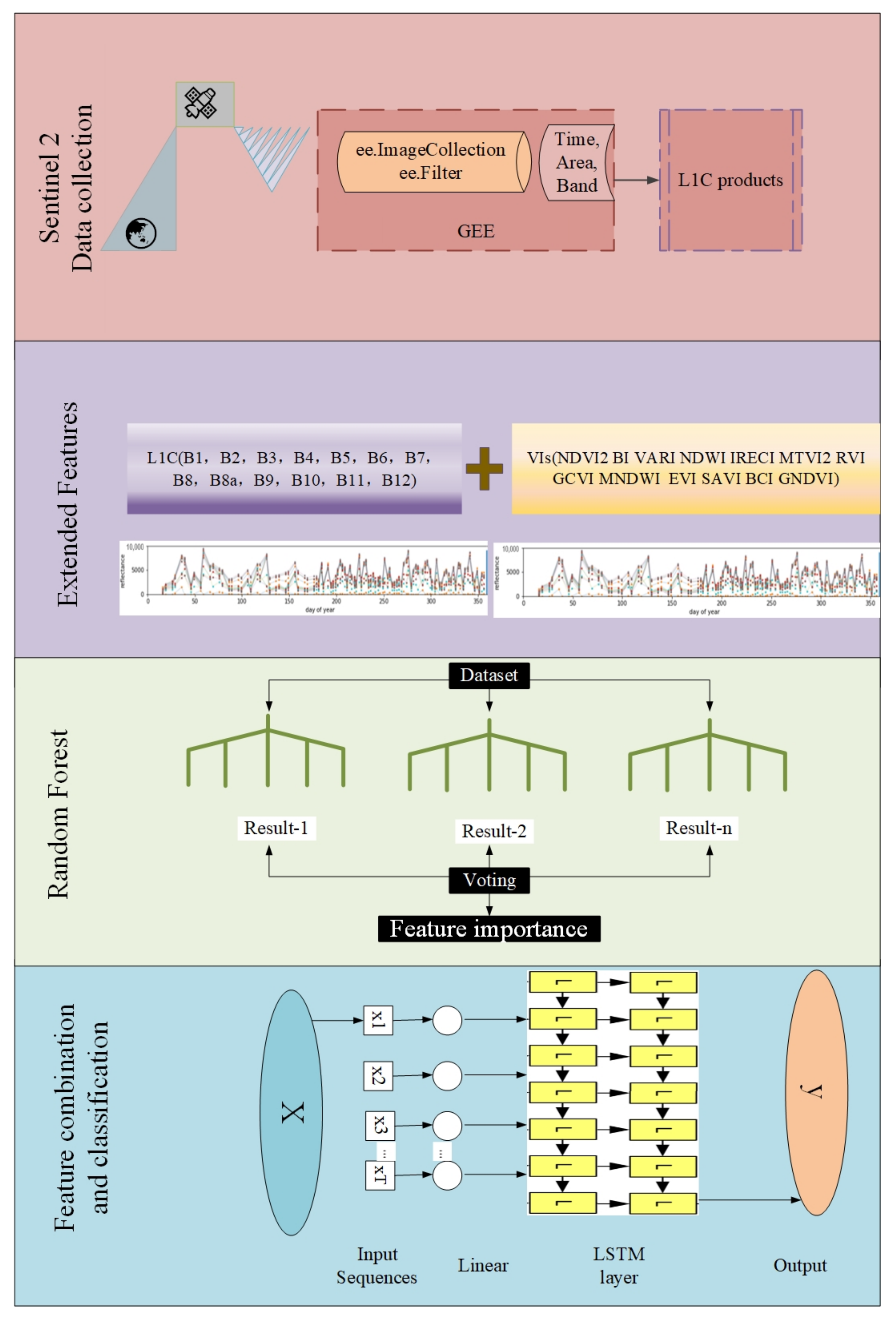
• Feature optimization: vegetation index features such as the normalized vegetation water index (NDWI), ratio vegetation index (RVI), enhanced vegetation index (EVI), and brightness index (BI) have been added to expand the features of each L1C band in the original time series. Then, the RF have been used to score the importance of features, and the important features of each time series have been selected to form a new dataset.
• Classification: Use an end-to-end deep learning model, a two-layer unidirectional LSTM, for training.

It is illustrated in Figure 1.

2. Study Areas and Data

2.1. Study Areas

There are two main sources of the dataset. The first study area is a 28 K plot in Bavaria in Upper Franconia of Germany, which is located in the south of Germany and covers an area of 1400 square kilometers. The region has a temperate continental climate with an average annual temperature of around 7° and a mean annual precipitation of 500 mm.

The second study area is a 580 K plot in the Brittany of France, which is located in the northwest of France and covers an area of 27,200 square kilometers. The region has a temperate maritime climate with mean annual temperatures ranging from 5.6° in winter to 17.5° in summer and mean annual precipitation of 650 mm. In particular, because of the large area of the study area, according to the division of the European Union administrative region, it is divided into four regions frh01, frh02, frh03, and frh04 respectively.

2.2. Data

S2 comprises twin polar-orbiting satellites in the same orbit, phased at 180 degrees to each other. Benefiting from the heritage of SPOT and LANDSAT missions, it will monitor variability in land surface conditions, and its wide swath width and high revisit time (10 days with one satellite at the equator, and 5 days with two satellites under cloud-free conditions, which results in 2–3 days at mid-latitudes) will support monitoring of vegetation changes within the growing season. The coverage is between latitudes 56° south and 84° north.

Moreover, the L1C product consists of 100 square kilometers of tiles, orthogonal images in the UTM/WGS84 projection. Using a digital elevation model in the mapping coordinates projection image L1C products. The survey provides all parameters of the top-of-atmosphere (TOA) reflectivity and converts them to radiation. According to the spectral resolution of different regions, the L1C product is resampled at 10, 20, and 60 m at a constant horizontal ground sampling distance.

Generally, the L1C processing includes radiometric correction and geometric correction. The S2 on L1C process is mainly broken into the following steps: tile association, heavy sampling grid computing and mask calculation. One purpose of this article is to challenge the original data and obtain robust classification results. Through the study of relatively primitive metadata, it is expected that agnostic areas without specific expert knowledge can be well classified in the future. Although the advantage of L2A data is that they have been atmospherically corrected and provide more accurate reflectance values, L1C as the top-of-atmosphere reflectance is more suitable for the research purpose of this article and can better realize the effective use of earth observation data without more complex processing flow.

The data in the study areas are organized in a manner in which the study areas are divided into regular plots, and the average value of reflectance data of all pixels in a certain band in each plot represents the value of this plot in this band. In that regard, a vector containing 13 values is formed, which is the mathematical expression of this plot at a certain time point. Here is the mathematical representation of this vector

$$x_t=({\rho }_{B1},{\rho }_{B2},{\rho }_{B3},{\rho }_{B4},{\rho }_{B5},{\rho }_{B6},{\rho }_{B7},{\rho }_{B8},{\rho }_{B8a},{\rho }_{B9},{\rho }_{B10},{\rho }_{B11},{\rho }_{B12})$$

(1)

where t is the day of the year, and ${\rho }_{B1}$ is noted as the reflectance of the $B1$ band, the rest are the same way. Some x chronologically forms the X, which is the mathematical representation of a plot or a sample,

$$X=\left(x_1,x_2,x_3,\dots \dots x_t\right)$$

(2)

This X is the TOA satellite data collected by S2 for one plot in one year, and many such X form the above two datasets, which are also the time series input to the model of this work.

The entire study area is divided into plots according to crop categories. Each plot is a crop category denoted by X and corresponds to the satellite image data of this plot. Namely, an X is a vector that represents a sample or crop. Furthermore, the X is that pixels within the plot are mean aggregated into a single feature vector of 13 spectral bands at each time. The length of this vector is the sequence length. In a more general sense, the sequence length is the number of days in a year that this sample is effectively observed to classify by satellites. The aforementioned items are illustrated in Figure 2.

It can be seen that a significant benefit of the L1C data is easy to obtain, but it not seem that it is easy to classify. In the original time series, most of the information from the measured signal is retained. However, at the same time, some phenological phenomena are obscured by noise caused by the atmosphere and clouds, which makes the data’s features full of ambiguity. Therefore, it has become essential to perform feature selection and analysis on the raw satellite data.

3. Methods

3.1. Sample Composition

The two areas provide crop-type time series labeled in the study fields. The first named BavarianCrops covers 7 common crops, including meadow, summer barley, corn, winter wheat, winter barley, clover, and winter triticale. There are 16,600 samples as a training set, 3057 samples as a validation set, and 7813 samples as a testing set, of which the dates are taken from 1 January to 31 December of 2018. The label data for the samples originate from a cooperation project with the Bavarian State Ministry of Food, Agriculture, and Forestry (StMELF) and the German remote sensing company GAF AG.

Although the second named BreizhCrops covers 9 crops, there exist some extensive definitions and minor samples resulting in less meaningful to achieve the significant classification. Only a subset is selected in this work. Therefore, this work has selected barley, wheat, rapeseed, corn, sunflowers, orchards, nuts, permanent grass, and temporary grass totaling 9 crops as the second. Meanwhile, there are 21,000 samples from frh01 and frh02, respectively, as a training set, 4000 samples from frh03 as a validation set, and 3000 samples from frh04 as a testing set, of which the dates are taken from 1 January to 31 December of 2017. Among them, sunflowers and nuts as infrequent classes are merely gathered four or five. While permanent grass and temporary grass take up the largest number to train the model. Collect and organize labels from the European Crop Subsidy Program. The two crop datasets have been shown in

Table 2. The two crop datasets used in the article are explained here. The content includes the name of the two datasets, the number of training sets, validation sets, and test sets used in each dataset, as well as the name and number of categories.

	Train	Validate	Test	Crops
BavarianCrops	16,600	3057	7813	7: meadow, summer barley, corn, winter, wheat, winter barley, clover, and winter triticale.
BreizhCrops	21,000	4000	3000	9: barley, wheat, rapeseed, corn, sunflowers, orchards, nuts, permanent grass, and temporary grass

.

3.2. Extended Features

The dataset used in this work is L1C of S2, which is lacking atmospheric correction and cloud obscuration operations. On the one hand, these disturbances make visual interpretation difficult, and on the other hand, they also make the features learned by the model less efficient. Therefore, on the basis of the original 13 spectral bands, the linear and nonlinear combination has been carried out to expand the other 13 VIs, with the purpose of mitigating the interference of atmosphere and clouds to different degrees to optimize the characteristics.

These 13 VIs mainly enhances characterization in the near-infrared, blue-wave, and green-wave bands. This is because of their important role in vegetation RS. The reflection in the near-infrared region is controlled by the complex cavity structure in the leaf and the multiple scattering of near-infrared radiation in the cavity. With the growth and development of plants or the state of stress by diseases and insect pests or the state of water deficit, the chlorophyll content of plant leaves, the tissue structure of leaf cavity, and the water content will all change, resulting in changes in the spectral characteristics of leaves. Although this change occurs simultaneously in the visible and near-infrared regions, the reflectance change is more pronounced in the near-infrared. This is very valuable for the distinction of plants or non-plants, the identification of different vegetation types, and the monitoring of vegetation growth.

After the NDVI is processed by ratio, it can partially eliminate the influence of solar altitude angle, satellite observation angle, terrain change, cloud shadow, and atmospheric attenuation. At the same time, the normalization processing of the NDVI can reduce the influence of remote sensor calibration fading on a single band and reduce the angle influence caused by surface two-way reflection and atmospheric effect. Therefore, the NDVI enhances the responsiveness to vegetation. In addition, its value range also determines that it is especially suitable for large-scale vegetation dynamic monitoring such as the world or continents. And an additional constant term is included in the denominator to account for atmospheric and background noise. This can help improve the accuracy of VIs for atmospheric disturbances or areas of low vegetation cover. The purpose of calculating the BI is to analyze vegetation trends over time, assess crop health and stress, and monitor land use changes in a given area. The normalized difference water index (NDWI) is used to study vegetation moisture and soil moisture, etc. Compared to other indices, the green normalized difference vegetation index (GNDVI) more accurately measures chlorophyll content to monitor vegetation in mature stages. The soil-adjusted vegetation index (SAVI) mitigates the impact of soil brightness, being particularly useful for the analysis of young crops. All of the VIs are selected and shown in

Table 3. Here is an introduction to the calculation methods and resolutions of the thirteen expanded VIS feature variables used in the article, which are constructed by the thirteen S2 bands.

Feature Variables	Calculation Formula	Resolution (m)
NDVI2 [24]	$NDVI2=\frac{(B8-B4)}{(B8+B4+0.1)}$	10
BI [23]	$BI=\sqrt{\frac{2\times {B4}^2}{{B3}^2}}$	10
VARI [25]	$VARI=\frac{(B3-B4)}{(B3+B4-B2)}$	10
NDWI [26]	$NDWI=\frac{(B8-B8a)}{(B8+B8a)}$	20
IRECI [23]	$IRECI=\frac{(b7-b4)\times b6}{B5}$	20
MTVI2 [27]	$MTVI2=\frac{1.5\ast \left(1.2\ast \left(B8-B3\right)-2.5\ast \left(B5-B3\right)\right)}{\sqrt{{\left(2\times B8+1\right)}^2-6\times B5+5\times B3+0.5}}$	20
RVI [25]	$RVI=\frac{B8}{B4}$	10
GCVI [28]	$GCVI=\frac{B4}{B3}-1$	10
MNDWI [29]	$MNDWI=\frac{(B3-B11)}{(B3+B11)}$	20
EVI [30]	$EVI=\frac{2.5\times (B8-B4)}{B8+6\times B4-7.5\times B2+1}$	10
SAVI [31]	$SAVI=\frac{1.5\times (B8-B4)}{(B8+B4+0.5)}$	10
BCI [32]	$BCI=0.1360\times B3+0.2611\times B4+0.3895\times B8$	10
GNDVI [33]	$GNDVI=\frac{(B8-B3)}{(B8+B3)}$	10

.

3.3. Feature Importance Optimization

There are two approaches to ensemble learning. One is boosting and the other is bagging. Random forest (RF) as a bagging algorithm composed of decision trees is popular in remote sensing [34,35,36]. Before introducing RF, it needs to mention the decision tree. The decision tree is a simple algorithm of supervised learning based on the if-then-else rule. It has strong interpretability and is also in line with human intuitive thinking. Notably, RF is composed of many decision trees without correlation. When performing classification tasks, the decision trees in the forest are allowed to judge and classify separately after a new input sample comes in and its classification result is obtained. Subsequently, the RF will decide the final result according to the most decision trees.

RF highlights two advantages. One is that it can balance the error for the unbalanced class. Another is that the importance of the features can be ranked, which is the direct cause why this paper chooses it from a series of the characteristics of the explanatory algorithm. Specifically, the Gini coefficient has been selected to evaluate the contribution of each feature on each tree in the RF, then take the average, and finally compare the contribution between features. Meanwhile, the method of cross-validated features has been implemented to validate the result of RF.

Conveniently, it can build and apply RF models by importing RandomForestClassifier from the scikit-learn library, a Python library that provides a rich set of machine-learning algorithms. And through the statement $rf.feature\_importances\_$, the feature importance ranking is obtained. Specifically, the RF model splits each feature, and then the reduction in the Gini index of each feature split is calculated. Finally, the greater the reduction in the Gini index after feature splitting, the greater the contribution of the feature to improving the purity of the dataset to highlight the higher the importance of the feature.

A set of parameters is configured for the behavior of a random forest classifier. $Bootstrap$ determines whether bootstrap samples are used when building individual decision trees in the RF. When $Bootstrap=False$, the entire dataset is used to build each tree. $Max\_depth$ controls the maximum depth of each decision tree in the random forest. Fixing it to the same length as the sequence length of the model to limit the number of levels in the tree can help prevent overfitting. $N\_estimators$ determines the number of decision trees in the RF ensemble. This work uses 2000 due to the considerable number of samples.

3.4. Classifier

In this paper, a method based on deep learning is applied to extract information from crop data. Namely, input data from the optimization of RF are reflected in feature maps and formalized as an objective function to obtain the signals. All this should be entirely due to the LSTM. Generally, the size of the training data is usually fixed to three dimensions containing batch sizes, sequence lengths, and feature numbers. Time series data has been ingested one observation at a time to get the output y by the model $f_{\theta }$. The LSTM introduces three gate mechanisms [37,38] controlling the flow and loss of information. There are input ($i_t$), forget ($f_t$), and output ($o_t$) gates, in addition to the introduction of a cell state representing long-term memory ($c_t$),

$$i_t=\sigma (W_{ii}{x}_t+b_{ii}+W_{hi}{h}_{t-1}+b_{hi})$$

(3)

$$f_t=\sigma (W_{if}{x}_t+b_{if}+W_{hf}{h}_{t-1}+b_{hf})$$

(4)

$$o_t=\sigma (W_{io}{x}_t+b_{io}+W_{ho}{h}_{t-1}+b_{ho})$$

(5)

$$c_t=f_t\odot c_{t-1}+i_t\odot g_t$$

(6)

$$h_t=o_t\odot tanh\left(c_t\right)$$

(7)

where $x_t$ is the input at present, ⊙ is the element-wise product. Here, W and b represent the weight matrix and bias, respectively, $c_t$ is functioned by $g_t=tanh(W_{ig}{x}_t+b_{ig}+W_{hg}{h}_{t-1}+b_{hg})$. The activation functions, $\delta \mathrm{and}tanh$, control the results range from 0 to 1 and −1 to 1 separately. Moreover, $h_t$ is obtained from the current cell state through the output gate, which characterizes the short-term memory. So, $c_{t-1}\mathrm{and}{h}_{t-1}$ are the state at the last moment.

Furthermore, the two output heads are functions of the hidden state of the layer $h_t$. One is used to calculate the classification probability to get the class,

$${\widehat{y}}_t=softmax\left(f_{{\theta }_c}\left(h_t\right)\right),$$

(8)

where the softmax function can then transform the multiclass output values into a probability distribution of with sum of 1. The other is used to calculate the scalar to stop the classification decision,

$$d_t=\sigma \left(f_{{\theta }_d}\left(h_t\right)\right).$$

(9)

Here, the $\sigma$ symbols a sigmoid function, which will scale the output to between 0 and 1.

It is indispensable to add the two tips before feeding the data to the model. Firstly, Layer Normalization (LN) [39] is added to standardize all inputs of each neuron in one layer to reduce the correlation between features, which simplifies model training and improves the accuracy of the model. It is similar to batch normalization except greatly focuses more on the standardization of each sample. Secondly, the linear layer linearly maps the input feature dimension to the hidden layer dimension of the model, which can also improve the accuracy of the model, as illustrated in Figure 3.

3.5. Experimental Design

The experiment of this paper is to complete the training and testing on a GeForce RTX 3090. The parallel computing engine adopts Nvidia’s CUDA version 11.6.55. Then, the two datasets were applied for classification. The experimental design of this study is as follows. Firstly, the overall accuracy of classification using the original and extended datasets is compared using LSTM. Next, the overall accuracy of classification using the extended feature dataset is observed at different sequence lengths. Then, after the extended features are ranked by RF, they are reordered and combined at the optimal observed sequence length and the overall accuracy of classification is observed. Simultaneously, cross-validation is performed on the results of this feature arrangement and combination. Finally, the performance of early prediction by the model is validated.

3.6. Metrics for Model’s Performance

The following metrics can be used to evaluate the performance and accuracy of a crop classification model. Mainly, overall accuracy measures the percentage of accurately classified instances in the classification results. Additionally, some metrics provide a comprehensive understanding of the model’s performance, including precision, recall, fscore, and kappa.

4. Experimental Results

In this work, to achieve robust classification of raw time series data without region-specific expert knowledge using satellite data released daily, a series of experiments were conducted to evaluate model accuracy on time series raw data and extended data. Before that, we uniformly set experimental conditions with 256 batch sizes and 100 epochs. Additionally, the origin learning and dropout rate of the LSTM model is $1\times {10}^{-3}$ and 0.2. Four indicators of accuracy metrics are emphasized: precision, recall, f-score, and kappa, to evaluate the model performance. Accuracy and earliness are the same components for attention.

4.1. Applicability of Extended Features

We conducted preliminary experiments to explore the overall accuracy (OA) of the classification of the original dataset and the extended dataset at a sequence length of 70. The OA of 0.86 and 0.80 can be obtained on the original dataset, while the OA of 0.87 and 0.80 can be obtained after adding features. Unexpectedly, the average growth rate of the extended BreizhCrops seems not to be improved. This is because only part of the BreizhCrops described in 3.2 was used in this paper. However, the original L1C samples of BreizhCrops are distributed in the four regions frh01, frh02, frh03, and frh04, in which the collected samples are 178,613, 140,645, 166,391, and 158,338 in turn. Such a large training sample often tended to take several hours to complete training, while the selected subset took only a few minutes to achieve the same overall training accuracy. As a result, not only the training time is greatly shortened, but also the training accuracy is consistent with the original large sample to prove the effectiveness of the algorithm.

4.2. Accuracy of Extended Features across Sequence Lengths

To adapt to the fact that only a small number of available time series can be obtained in some areas, the sample size of the input model is reduced. That is, under different sequence lengths, the minimum sequence length can be explored while maintaining high classification accuracy. At the same time, it reduces the computational burden of the model.

Figure 4 shows the error plot of OA of BavarianCrops and BreizhCrops in different time series after expanding features. The meaning of y is the mean of OA obtained after the same experiment repeated ten times at each sequence.

We carefully observe the relationship between sequence length and classification accuracy. On the left, when the sequence length is 65, the OA reaches 0.87. In contrast, on the right, when the sequence length is 50, the OA can get 0.8. Nevertheless, when the sequence length continues to grow longer, the lack of information on sunflowers and nuts, highly imbalanced classes in BreizhCrops, leads to the limited ability of the model to learn. Furthermore, the generalization performance of the whole model is slashed, and the classification performance is worse. As mentioned before, this is vividly demonstrated in Figure 4.

Overall, the results show the possibility of downsizing the sequence length. Expanding features based on the original data can make the sample data gain adaptability in sequence length.

4.3. Feature Ranked by RF at Optimal Sequence Lengths

The RF model is a powerful ensemble learning model consisting of multiple decision trees, which can be used to solve classification and regression problems. Importantly, RF can explain the importance of features. In this part, after feature importance ranking by RF, we recombined features to train the model at the minimum sequence length.

Table 4. Recognition accuracy of the two datasets in their own minimum sequence length with different combinations selected features by RF.

	BavarianCrops	Feature Combinations	Feature Numbers	OA
Sequencelength
65		[B1, B10, B11, B12, B2, B3, B4, B5, B6, B7, B8, B8A, B9, NDVI2, BI, VARI, NDWI, IRECI, MTVI2, RVI, GCVI, MNDWI, EVI, SAVI, BCI, GNDVI]	26	0.8760
65		[B1, B10, B11, B12, B2, B3, B4, B5, B6, B7, B8A, B9, NDVI2, BI, VARI, NDWI, IRECI, MTVI2, RVI, GCVI, MNDWI, EVI, SAVI, BCI, GNDVI]	25	0.8639
65		[B1, B10, B11, B12, B2, B3, B4, B5, B6, B7, B8A, B9, NDVI2, BI, VARI, NDWI, IRECI, MTVI2, RVI, GCVI, MNDWI, EVI, SAVI, GNDVI]	24	0.8617
65		[B1, B10, B11, B12, B2, B3, B4, B5, B6, B7, B8A, B9, NDVI2, BI, VARI, NDWI, IRECI, MTVI2, RVI, GCVI, MNDWI, EVI, GNDVI]	23	0.8534
65		[B1, B10, B11, B12, B2, B3, B4, B5, B6, B7, B8A, B9, NDVI2, BI, VARI, NDWI, IRECI, MTVI2, RVI, GCVI, MNDWI, EVI]	22	0.8541
65		[B1, B10, B11, B12, B2, B3, B4, B5, B6, B7, B9, NDVI2, BI, VARI, NDWI, IRECI, MTVI2, RVI, GCVI, MNDWI, EVI]	21	0.8582
65		[B1, B10, B11, B12, B2, B3, B4, B5, B6, B7, B9, NDVI2, BI, VARI, NDWI, MTVI2, RVI, GCVI, MNDWI, EVI]	20	0.8616
65		[B1, B10, B11, B12, B2, B4, B5, B6, B7, B9, NDVI2, BI, VARI, NDWI, MTVI2, RVI, GCVI, MNDWI, EVI]	19	0.8600
65		[B1, B10, B11, B12, B2, B4, B5, B6, B7, B9, NDVI2, BI, NDWI, MTVI2, RVI, GCVI, MNDWI, EVI]	18	0.8513
65		[B1, B10, B11, B12, B2, B4, B5, B6, B9, NDVI2, BI, NDWI, MTVI2, RVI, GCVI, MNDWI, EVI]	17	0.8662
65		[B1, B10, B11, B12, B2, B4, B5, B9, NDVI2, BI, NDWI, MTVI2, RVI, GCVI, MNDWI, EVI]	16	0.8623
65		[B1, B10, B11, B12, B2, B4, B9, NDVI2, BI, NDWI, MTVI2, RVI, GCVI, MNDWI, EVI]	15	0.8613
65		[B1, B10, B11, B12, B4, B9, NDVI2, BI, NDWI, MTVI2, RVI, GCVI, MNDWI, EVI]	14	0.8563
65		[B1, B10, B11, B4, B9, NDVI2, BI, NDWI, MTVI2, RVI, GCVI, MNDWI, EVI]	13	0.8593
65		[B1, B10, B11, B4, B9, NDVI2, BI, MTVI2, RVI, GCVI, MNDWI, EVI]	12	0.8521
50		[B1, B10, B11, B12, B2, B3, B4, B5, B6, B7, B8, B8A, B9, NDVI2, BI, VARI, NDWI, IRECI, MTVI2, RVI, GCVI, MNDWI, EVI, SAVI, BCI, GNDVI]	26	0.8000
50		[B1, B10, B11, B12, B2, B3, B4, B5, B6, B7, B8A, B9, NDVI2, BI, VARI, NDWI, IRECI, MTVI2, RVI, GCVI, MNDWI, EVI, SAVI, BCI, GNDVI]	25	0.7962
50		[B1, B10, B11, B12, B2, B3, B4, B5, B6, B7, B8A, B9, NDVI2, BI, VARI, NDWI, IRECI, MTVI2, RVI, GCVI, MNDWI, EVI, SAVI, GNDVI]	24	0.7960
50		[B1, B10, B11, B12, B2, B3, B4, B5, B6, B7, B8A, B9, NDVI2, BI, VARI, NDWI, IRECI, MTVI2, RVI, GCVI, MNDWI, EVI, GNDVI]	23	0.7913
50		[B1, B10, B11, B12, B2, B3, B4, B5, B6, B7, B8A, B9, NDVI2, BI, VARI, NDWI, IRECI, MTVI2, RVI, GCVI, MNDWI, EVI]	22	0.7820
50		[B1, B10, B11, B12, B2, B3, B4, B5, B6, B7, B9, NDVI2, BI, VARI, NDWI, IRECI, MTVI2, RVI, GCVI, MNDWI, EVI]	21	0.7801
50		[B1, B10, B11, B12, B2, B3, B4, B5, B6, B7, B9, NDVI2, BI, VARI, NDWI, MTVI2, RVI, GCVI, MNDWI, EVI]	20	0.7763
50		[B1, B10, B11, B12, B2, B4, B5, B6, B7, B9, NDVI2, BI, VARI, NDWI, MTVI2, RVI, GCVI, MNDWI, EVI]	19	0.7712
50		[B1, B10, B11, B12, B2, B4, B5, B6, B7, B9, NDVI2, BI, NDWI, MTVI2, RVI, GCVI, MNDWI, EVI]	18	0.7709
50		[B1, B10, B11, B12, B2, B4, B5, B6, B9, NDVI2, BI, NDWI, MTVI2, RVI, GCVI, MNDWI, EVI]	17	0.7660
50		[B1, B10, B11, B12, B2, B4, B5, B9, NDVI2, BI, NDWI, MTVI2, RVI, GCVI, MNDWI, EVI]	16	0.7615
50		[B1, B10, B11, B12, B2, B4, B9, NDVI2, BI, NDWI, MTVI2, RVI, GCVI, MNDWI, EVI]	15	0.7596
50		[B1, B10, B11, B12, B4, B9, NDVI2, BI, NDWI, MTVI2, RVI, GCVI, MNDWI, EVI]	14	0.7563
50		[B1, B10, B11, B4, B9, NDVI2, BI, NDWI, MTVI2, RVI, GCVI, MNDWI, EVI]	13	0.7523
50		[B1, B10, B11, B4, B9, NDVI2, BI, MTVI2, RVI, GCVI, MNDWI, EVI]	12	0.7500

indicates the classification performance.

Moreover, this paper also set up an automatic cross-validation feature experiment, namely, selecting features automatically for the model to obtain classification accuracy. Then the training results of automatic verification on input features confirm that extended features and feature optimization can improve the classification illustrated in Figure 5.

Ranking of feature importance according to RF, one feature with the lowest score is subtracted in turn, and the classification accuracy of the remaining feature combinations is observed. On the BavarianCrops dataset, while gradually reducing the number of features, OA is also slowly decreasing. Moreover, on the BreizhCrops dataset, OA shows the same transformation trend. Although classification is performed at the optimal length of time, OA will be affected when reducing the number of features, which illustrates the difference in model performance caused by different feature arrangements. A cross-validation on random feature combinations also verified this. The last observed features include vegetation indices such as MNDWI, NDVI2, BI, MTVI2, RVI, GCVI, EVI, and spectral bands B1, B10, B11, B4, and B9. It is not difficult to notice that these indices are mainly distributed in different kinds of red light bands, which can be used to represent the health of crops.

Overall, the recombined features verify the improvement of the model classification performance through the extended features. In other words, the extended features provide additional information to complement the original features, which may be a reference for the process of L1C data.

4.4. Availability of Early Prediction

In addition to the end-to-end classification based on the model in this paper, the ability to make classification decisions in advance according to time series is also considered. Meanwhile, the above experiments consider the performance of the model to decide to stop classification. Next, early predictions are illustrated through experimental results trained with minimum sequence length in Figure 6 and Figure 7, and

Table 5. Accuracy metrics of crop classification in the minimum sequence length.

Dataset	Minimum Sequence Length	Precision	Recall	Fscore	Kappa
BavarianCrops	65	0.796	0.735	0.754	0.815
BreizhCrops	50	0.552	0.535	0.540	0.734

.

Figure 6 shows the distribution of the time when BavarianCrops and BreizhCrops stop classification for each category. In comparison, the decision time of each category of BavarianCrops is slightly later than that of BreizhCrops. However, it is noted that BreizhCrops has a larger number of samples than BavarianCrops in every category except for the small sample category. Figure 7 showcases the probability that the two datasets can be classified at a certain minimum sequence length. Due to the much more significant than BavarianCrops, BreizhCrops has an early possibility. Table 5 records the accuracy of the model.

The availability of early prediction has been substantiated due to a $d_t$ function introduced by the proposed method in the LSTM output to select an appropriate sequence length. Precisely, when the value of the $d_t$ function rapidly changes from 0 to 1, the required sequence length corresponds to the minimum number of observed days for early classification. This approach allows for prediction using the minimum number of effective observation days in validation samples or general real-world applications, thereby reflecting early prediction.

5. Discussion

Model’s Performance Comparison and Analysis

Based on the comparative study of the considerably relevant literature, LSTM, a model with the best performance in time series data classification, has been selected as the key to solving the problem. However, the selection has also been verified by setting up two controlled experiments in the whole dataset. The first group is implemented to classify data on RF and LSTM to compare the overall accuracy. The second group is implemented to classify data at the minimum sequence length on LSTM and RNN to compare the overall accuracy.

From

Table 6. Comparison of classification with RF and LSTM.

Dataset	Classifier	Sequence Length	Feature Numbers	OA	Fscore
BavarianCrops	RF	70	13	0.65	0.56
	LSTM	70	13	0.86	0.77
BreizhCrops	RF	70	13	0.62	0.61
	LSTM	70	13	0.80	0.74

, the result of directly using RF for classification is inferior to that of LSTM, which verifies that LSTM is more suitable for sequence problems. From

Table 7. Comparison of classification with RNN and LSTM at minimum sequence length.

Dataset	Classifier	Sequence Length	Feature Numbers	OA	Fscore
BavarianCrops	RNN	65	26	0.80	0.71
	LSTM	65	26	0.87	0.79
BreizhCrops	RNN	50	26	0.76	0.68
	LSTM	50	26	0.80	0.75

, the classification result of the RNN is not as good as that of LSTM at the minimum sequence length, which verifies the good classification performance of LSTM. It also confirms that the unidirectional LSTM is suitable for extracting crop growth characteristics in a year. That is to say, the input of LSTM used is only processed in a forward pass at a one-time step without utilizing information from subsequent time steps. The one-way processing is suitable for tasks where future information has little impact on current predictions.

There still exist some main limitations to resolve. Due to the lack of field sample data, the results could not be plotted into maps according to field coordinates. In addition, the proportion of samples between categories is unbalanced. For example, the number of samples of the ordinary crop corn is significantly greater than that of the rare clover. Thus, it leads to bias in the classification of categories with sample sizes like clover in the single digits.

There are inconsistencies in the effectively observed days to classify by satellites in the original data, which leads to differences in sample quality. Not only use extended features to enrich the data but also use the minimum number of valid observation days for classification as much as possible. From the experimental results, the proposed method meets the above requirements. In the future, it is still believed to be possible to achieve robust classification of sample data without expert knowledge.

6. Conclusions

We process the TOA reflectance values data of S2 by feature extended and importance optimization so that the OA of end-to-end crop classification based on LSTM is improved. Specifically, starting from the disadvantage of L1C data, a total of 13 features have been organized to alleviate the impact of its disadvantage, which include 3 categories, namely vegetation indices, soil indices, and water indices. Then, the importance of all features is ranked by RF to explain the importance of features. In addition, it is validated using the method of cross-validated features. Finally, the features are fed into the model for end-to-end classification. Although the used Breizhcrop has fewer data than the original Breizhcrop, the experimental results show that the classification accuracy is consistent and the training speed is fast, which reflects the superiority of this work. Furthermore, since the actual planting area of the nine classes of sunflower and nuts is small, only four to five training samples are available, which affects the classification accuracy. Yet from the OA, the proposed method has offset part of the influence. However, in the case where each category of the main training set is a large sample, it is still a challenging task for the training mode with few samples.

Achieving an accurate classification of the available satellite data is what this work is about. Feature optimization overcomes data quality and bulk challenges, enabling robust classification of raw time series data without region-specific expert knowledge. An end-to-end classification method is a powerful tool for crop documentation and policy development.

References

1. Wulder, M.A.; Roy, D.P.; Radeloff, V.C.; Loveland, T.R.; Anderson, M.C.; Johnson, D.M.; Healey, S.P.; Zhu, Z.; Scambos, T.A.; Pahlevan, N.; et al. Fifty years of Landsat science and impacts. Remote Sens. Environ. 2022, 228, 113195. [Google Scholar] [CrossRef]
2. Emery, W.; Camps, A. Chapter 10—Land Applications. In Introduction to Satellite Remote Sensing; Emery, W., Camps, A., Eds.; Elsevier: Amsterdam, The Netherlands, 2017; pp. 701–766. [Google Scholar] [CrossRef]
3. Tong, X.; Zhao, W.; Xing, J.; Fu, W. Status and development of China High-Resolution Earth Observation System and application. In Proceedings of the 2016 IEEE International Geoscience and Remote Sensing Symposium (IGARSS), Beijing, China, 10–15 July 2016; pp. 3738–3741. [Google Scholar] [CrossRef]
4. Liang, S. (Ed.) 8.01—Volume 8 Overview: Progress in Ocean Remote Sensing. In Comprehensive Remote Sensing; Elsevier: Oxford, UK, 2018; pp. 1–42. [Google Scholar] [CrossRef]
5. Schumann, G.J.P. (Ed.) Chapter 2—An Automatic System for Near-Real Time Flood Extent and Duration Mapping Based on Multi-Sensor Satellite Data. In Earth Observation for Flood Applications; Earth Observation; Elsevier: Amsterdam, The Netherlands, 2021; pp. 7–37. [Google Scholar] [CrossRef]
6. Martimort, P.; Arino, O.; Berger, M.; Biasutti, R.; Carnicero, B.; Del Bello, U.; Fernandez, V.; Gascon, F.; Greco, B.; Silvestrin, P.; et al. Sentinel-2 optical high resolution mission for GMES operational services. In Proceedings of the 2007 IEEE International Geoscience and Remote Sensing Symposium, Barcelona, Spain, 23–27 July 2007; pp. 2677–2680. [Google Scholar] [CrossRef]
7. Zhang, X.; Liu, J.F.; Qin, Z.; Qin, F. Winter wheat identification by integrating spectral and temporal information derived from multi-resolution remote sensing data. J. Integr. Agric. 2019, 18, 2628–2643. [Google Scholar] [CrossRef]
8. Arvor, D.; Jonathan, M.; Meirelles, M.S.P.; Dubreuil, V.; Durieux, L. Classification of MODIS EVI time series for crop mapping in the state of Mato Grosso, Brazil. Int. J. Remote Sens. 2011, 32, 7847–7871. [Google Scholar] [CrossRef]
9. Salvatore Praticò, S.; Solano, F.; Di Fazio, S.; Modica, G. Machine Learning Classification of Mediterranean Forest Habitats in Google Earth Engine Based on Seasonal Sentinel-2 Time-Series and Input Image Composition Optimisation. Remote Sens. 2021, 13, 586. [Google Scholar] [CrossRef]
10. Peñá-Barragán, J.M.; Ngugi, M.K.; Plant, R.E.; Six, J. Object-based crop identification using multiple vegetation indices, textural features and crop phenology. Remote Sens. Environ. 2011, 115, 1301–1316. [Google Scholar] [CrossRef]
11. Brown, J.C.; Kastens, J.H.; Coutinho, A.C.; de Castro Victoria, D.; Bishop, C.R. Classifying multiyear agricultural land use data from Mato Grosso using time-series MODIS vegetation index data. Remote Sens. Environ. 2013, 130, 39–50. [Google Scholar] [CrossRef]
12. Zeng, L.; Wardlow, B.D.; Xiang, D.; Hu, S.; Li, D. A review of vegetation phenological metrics extraction using time-series, multispectral satellite data. Remote Sens. Environ. 2020, 237, 111511. [Google Scholar] [CrossRef]
13. Conrad, C.; Fritsch, S.; Zeidler, J.; Rücker, G.; Dech, S. Per-Field Irrigated Crop Classification in Arid Central Asia Using SPOT and ASTER Data. Remote Sens. 2010, 2, 1035–1056. [Google Scholar] [CrossRef]
14. Zhong, L.; Gong, P.; Biging, G.S. Efficient corn and soybean mapping with temporal extendability: A multi-year experiment using Landsat imagery. Remote Sens. Environ. 2014, 140, 1–13. [Google Scholar] [CrossRef]
15. Pelletier, C.; Webb, G.I.; Petitjean, F. Temporal Convolutional Neural Network for the Classification of Satellite Image Time Series. Remote Sens. 2019, 11, 523. [Google Scholar] [CrossRef]
16. Fawaz, H.I.; Lucas, B.; Forestier, G.; Pelletier, C.; Schmidt, D.F.; Weber, J.; Webb, G.I.; Idoumghar, L.; Muller, P.; Petitjean, F. InceptionTime: Finding AlexNet for Time Series Classification. arXiv 2019, arXiv:1909.04939. [Google Scholar]
17. Kussul, N.; Lavreniuk, M.; Skakun, S.; Shelestov, A. Deep Learning Classification of Land Cover and Crop Types Using Remote Sensing Data. IEEE Geosci. Remote Sens. Lett. 2017, 14, 778–782. [Google Scholar] [CrossRef]
18. Amato, F.; Guignard, F.; Robert, S.; Kanevski, M.F. A novel framework for spatio-temporal prediction of environmental data using deep learning. Sci. Rep. 2020, 10, 22243. [Google Scholar] [CrossRef] [PubMed]
19. Luo, C.; Meng, S.; Hu, X.; Wang, X.; Zhong, Y. Cropnet: Deep Spatial-Temporal-Spectral Feature Learning Network for Crop Classification from Time-Series Multi-Spectral Images. In Proceedings of the IGARSS 2020—2020 IEEE International Geoscience and Remote Sensing Symposium, Waikoloa, HI, USA, 26 September–2 October 2020; pp. 4187–4190. [Google Scholar] [CrossRef]
20. Zhou, Y.; Luo, J.; Feng, L.; Yang, Y.; Chen, Y.; Wu, W. Long-short-term-memory-based crop classification using high-resolution optical images and multi-temporal SAR data. GISci. Remote Sens. 2019, 56, 1170–1191. [Google Scholar] [CrossRef]
21. Rußwurm, M.; Courty, N.; Emonet, R.; Lefèvre, S.; Tuia, D.; Tavenard, R. End-to-end learned early classification of time series for in-season crop type mapping. ISPRS J. Photogramm. Remote Sens. 2023, 196, 445–456. [Google Scholar] [CrossRef]
22. Rußwurm, M.; Lefèvre, S.; Körner, M. BreizhCrops: A Satellite Time Series Dataset for Crop Type Identification. arXiv 2019, arXiv:1905.11893. [Google Scholar]
23. Rußwurm, M.; Körner, M. Self-attention for raw optical Satellite Time Series Classification. ISPRS J. Photogramm. Remote Sens. 2020, 169, 421–435. [Google Scholar] [CrossRef]
24. Rouse, J.W.; Haas, R.H.; Schell, J.A.; Deering, D.W. Monitoring Vegetation Systems in the Great Plains with ERTS. 1974. Available online: https://ntrs.nasa.gov/citations/19740022614 (accessed on 1 January 2023).
25. EOS Data Analytics. 2022. Available online: https://eos.com/blog/vegetation-indices (accessed on 1 January 2023).
26. Gao, B.C. NDWI-A Normalized Difference Water Index for Remote Sensing of Vegetation Liquid Water from Space. Remote Sens. Environ. 1996, 58, 257–266. [Google Scholar] [CrossRef]
27. Haboudane, D.; Miller, J.; Pattey, E.; Zarco-Tejada, P.; Strachan, I. Hyperspectral vegetation indices and Novel Algorithms for Predicting Green LAI of crop canopies: Modeling and Validation in the Context of Precision Agriculture. Remote Sens. Environ. 2004, 90, 337–352. [Google Scholar] [CrossRef]
28. Gitelson, A.A.; Viña, A.; Arkebauer, T.J.; Rundquist, D.; Keydan, G.P.; Leavitt, B. Remote estimation of leaf area index and green leaf biomass in maize canopies. Geophys. Res. Lett. 2003, 30. [Google Scholar] [CrossRef]
29. Du, Y.; Zhang, Y.; Ling, F.; Wang, Q.; Li, W.; Li, X. Water Bodies Mapping from Sentinel-2 Imagery with Modified Normalized Difference Water Index at 10-m Spatial Resolution Produced by Sharpening the SWIR Band. Remote Sens. 2016, 8, 354. [Google Scholar] [CrossRef]
30. Huete, A.; Didan, K.; Miura, T.; Rodriguez, E.; Gao, X.; Ferreira, L. Overview of the Radiometric and Biophysical Performance of the MODIS Vegetation Indices. Remote Sens. Environ. 2002, 83, 195–213. [Google Scholar] [CrossRef]
31. Huete, A. A soil-adjusted vegetation index (SAVI). Remote Sens. Environ. 1988, 25, 295–309. [Google Scholar] [CrossRef]
32. Nedkov, R. Orthogonal transformation of segmented images from the satellite sentinel-2. Comptes Rendus L’Académie Bulg. Sci. Sci. Math. Nat. 2017, 70, 687–692. [Google Scholar]
33. Gitelson, A.; Kaufman, Y.; Merzlyak, M. Use of a green channel in remote sensing of global vegetation from EOS-MODIS. Remote Sens. Environ. 1996, 58, 289–298. [Google Scholar] [CrossRef]
34. Pasquarella, V.J.; Holden, C.E.; Woodcock, C.E. Improved mapping of forest type using spectral-temporal Landsat features. Remote Sens. Environ. 2018, 210, 193–207. [Google Scholar] [CrossRef]
35. Teluguntla, P.G.; Thenkabail, P.S.; Oliphant, A.J.; Xiong, J.; Gumma, M.K.; Congalton, R.G.; Yadav, K.; Huete, A.R. A 30-m landsat-derived cropland extent product of Australia and China using random forest machine learning algorithm on Google Earth Engine cloud computing platform. ISPRS J. Photogramm. Remote Sens. 2018, 144, 325–340. [Google Scholar] [CrossRef]
36. Pelletier, C.; Valero, S.; Inglada, J.; Champion, N.; Dedieu, G. Assessing the robustness of Random Forests to map land cover with high resolution satellite image time series over large areas. Remote Sens. Environ. 2016, 187, 156–168. [Google Scholar] [CrossRef]
37. Józefowicz, R.; Zaremba, W.; Sutskever, I. An Empirical Exploration of Recurrent Network Architectures. In Proceedings of the International Conference on Machine Learning, Lille, France, 6–11 July 2015. [Google Scholar]
38. Sak, H.; Senior, A.W.; Beaufays, F. Long Short-Term Memory Based Recurrent Neural Network Architectures for Large Vocabulary Speech Recognition. arXiv 2014, arXiv:1402.1128. [Google Scholar]
39. Ba, J.L.; Kiros, J.R.; Hinton, G.E. Layer Normalization. arXiv 2016, arXiv:1607.06450. [Google Scholar]
Figure 1. The overall method for crop classification.
Remotesensing 15 05203 g001
Figure 2. The study area is clearly marked on a map of the country. On the left, the German research area is located at the red dot marked on the map, while the four subdivisions frh01, frh02, frh03, and frh04 of Brittany in France, according to the European Union’s regional classification standard, are distributed as indicated by the pink blocks. On the right, it visualizes the meaning of a training sample X. According to the topography, a training sample X is a square-shaped land plot within the research region. Furthermore, it is the satellite observation data of a small plot.
Remotesensing 15 05203 g002
Figure 3. The model for crop classification. In the figure, 256 represents the size of the training batch at once, 70 is the sequence length of each sample, 26 is the number of expanded features, and 64 is the number of features represented by the LSTM hidden layer. Finally, the model outputs two tensors, one calculating the probability of the n categories that need to be classified, and the other calculating the probability that the classification can be hard stopped for that category.
Remotesensing 15 05203 g003
Figure 4. Performance of the extended features with a few sequence lengths. To analyze this, we examine the relationship between sequence length and OA by increasing the sequence length in increments of five units and observing the corresponding OA. By doing so, we can determine if increasing the number of features allows for a reduction in sequence length.
Remotesensing 15 05203 g004
Figure 5. Performance of the randomly cross-validated features. To analyze this, we examine the relationship between feature numbers and OA by just increasing the feature number in turn and observing the corresponding OA. By doing so, we validate if the trend in OA aligns with the results after applying RF.
Remotesensing 15 05203 g005
Figure 6. The relation is shown as boxplots between the samples in each category and the required sequence length when the model implements the decision to stop classification. The top shows the case of seven categories for BavarianCrops, while the bottom shows the case of nine categories for Breizhcrops. The samples that fall outside the box are outliers. The reason for the line on the right is that the nuts category belongs to the small sample with only one verification sample.
Remotesensing 15 05203 g006
Figure 7. The figure shows the probability that the model can stop classifying and make a classification decision given a certain sequence length. It can be seen that BavarianCrops tends to make the complete decision when the sequence length is 49 on the above, while BreizhCrops is 35 on the bottom.
Remotesensing 15 05203 g007