Article

Mapping Fractional Vegetation Cover Using Unoccupied Aerial Vehicle Imagery to Guide Conservation of a Rare Riparian Shrub Ecosystem in Southern California

1
Department of Geography, San Diego State University, San Diego, CA 92182, USA
2
Department of Botany and Plant Sciences, University of California Riverside, Riverside, CA 92521, USA
3
Department of Geography, California State University Long Beach, Long Beach, CA 90840, USA
*
Author to whom correspondence should be addressed.
Remote Sens. 2023, 15(21), 5113; https://doi.org/10.3390/rs15215113
Submission received: 19 September 2023 / Revised: 16 October 2023 / Accepted: 20 October 2023 / Published: 26 October 2023
(This article belongs to the Section Remote Sensing in Agriculture and Vegetation)

Abstract

:
The use of unoccupied aerial vehicles (UAVs) for vegetation monitoring is widespread in agriculture and forestry but far less so in ecological restoration where it has tremendous unrealized potential. We tested the ability of multispectral data and a derived vegetation index to classify shrub, herbaceous vegetation, and bare soil cover in a rare alluvial floodplain vegetation community in semiarid Southern California, where shrub cover is manipulated in restoration efforts aimed to provide open habitats required by several threatened and endangered species. Three classifiers and three levels of spatial aggregation were compared for their ability to provide accurate shrub cover estimates at a scale commensurate with the needs of conservation managers. We used object-based image analysis (OBIA) and compared maximum likelihood (ML), support vector machine (SVM), and random forest (RF) classifiers applied to high-spatial resolution (0.14 m) data from a four-band Parrot Sequoia+ multispectral sensor. The SVM and RF classifiers yielded similarly high classification accuracy evaluated using the training data (overall accuracy of 96.4% and 97.6%, respectively), much higher than ML (88%). Aggregating shrub cover data to 25 and 50 m resolutions yielded more accurate and well-calibrated cover estimates (mean absolute error 12% and 11%, respectively, for RF) than 10 m aggregation (MAE 19% for RF). Shrub cover estimated using RF and SVM was able to meet the restoration monitoring needs to distinguish the three phases of shrub habitat characterized by their cover (10–30%, 30–75%, >75%) that differ in habitat quality and restoration prescriptions.

1. Introduction

Cost-effective, accurate methods for monitoring arid land riparian ecosystems in support of ecological management and conservation are urgently needed. Remotely sensed earth observations provide an opportunity for developing low-cost monitoring programs in both degraded and protected ecosystems that are targets for management efforts, significantly reducing the time and monetary costs associated with extensive field surveys. The popularity of cameras or sensors mounted on unoccupied aerial vehicles (UAVs, commonly referred to as “drones”) for environmental and ecological monitoring has increased due to their low cost and capacity to detect biological phenomena at relevant scales [1]. UAV imagery has been used for habitat mapping (spectral unmixing) [2], mapping the extent of invasive plant species [3], and monitoring post-disturbance vegetation recovery [4]. These tools provide a powerful opportunity for guiding ecological management decisions using consistent, multi-year data collection [5]. However, there is still a lack of clarity regarding the best methodological approaches for transforming UAV-collected data into usable information for on-the-ground ecologists [6].
Phinn et al. (2003) developed a framework for optimizing the use of remote sensing for ecological monitoring, wherein selecting the appropriate temporal, spatial, spectral, and classification parameters depends on the natural system being monitored as well as the management program’s objective [7]. A variety of remote sensing approaches have been developed in the context of this framework to advance ecological monitoring [8,9,10]. There is a significant opportunity to extend these approaches to similarly assess ecosystem recovery after management actions have been implemented [5]. Ecosystem restoration regularly implements actions to change vegetation structure and composition across a range of spatial scales to enhance physical conditions, ecosystem function, and structural diversity to support wildlife, where the success of these actions is assessed via an “ecosystem recovery wheel” [11]. Merging these two fields of ecological monitoring and ecological restoration provides land managers with a tool that works across conservation and management goals. Here, we tested two components of this framework that are often included in natural resource remote sensing projects: ground cover classification, and spatial scale for fractional cover mapping, in a rare and threatened riparian vegetation community in southern California. In the context of the ecosystem recovery wheel [5], the ecological attributes targeted in our case study are spatial mosaic, vegetation strata, habitat quality, and distinguishing desirable and undesirable plants.
Many projects that use remote sensing to monitor ecological phenomena require the implementation of supervised image classification, where pixels are assigned to specific land cover classes to create thematic maps. A variety of supervised classification approaches are frequently used for vegetation mapping based on remotely sensed imagery [12]. These approaches include conventional, parametric approaches, such as the maximum likelihood (ML) classifier, which was the most widely implemented method identified in a meta-analysis conducted in 2014, despite often having lower accuracy than machine learning methods [13]. However, in certain contexts (e.g., desert vegetation), ML has been found to perform as well or better than other classification methods [14]. With respect to machine learning approaches known for their ability to model complex phenomena without making assumptions about data distributions, random forest (RF) and support vector machine (SVM) are among the most advanced and easily implemented [15,16]. SVM is able to balance accuracy with the ability to generalize to new data [17] and can produce accurate classification results with relatively little training data [18]. RF is an ensemble machine learning technique [19] that combines multiple classifiers to obtain more accurate results via bootstrap aggregation. A comprehensive review suggested that SVM and RF are fairly evenly matched in terms of accuracy, especially for high-resolution data with few features (bands), with RF perhaps showing slightly better performance when classifying land cover/land use [20]. Because the performance of different classifiers is context-dependent and there is no “best” universal classifier, comparing the performance of different classification methods within a specific area of interest is an essential step for using remote sensing as an ecological management and monitoring tool.
Fractional vegetation cover is an important component of ecosystem health and is often used to detect vegetation change through time [21,22], making it a useful indicator to monitor the progress of ecological restoration [5]. However, grid-cell sizes used to estimate fractional vegetation cover differ in accuracy and mapped outputs, factors that may lead to different management and restoration outcomes. For example, research in a southern California coastal sage scrub (CSS) plant community found that aggregating fine-scale pixel-based classification to coarser 40 m grids yielded the lowest error and uncertainty, when compared to grid sizes of 20 m and 10 m [23]. The spatial sampling scale has been long recognized for its importance in investigating landscape patterns [24] and establishing the appropriate scale(s) for quantifying fractional cover in a particular system is imperative for informed management decision making [25].
We conducted our study in Riversidean alluvial fan sage scrub (RAFSS), a rare arid land riparian vegetation community found in Southern California that supports 24 sensitive animal and plant species, including the endangered San Bernardino kangaroo rat (Dipodomys merriami parvus; SBKR) and Santa Ana River Woolly Star (Eriastrum densifolium ssp. sanctorum; SARWS) [26]. This vegetation type consists of sparse woody and evergreen plant species distributed across complex terrain features that are created by flooding events, i.e., floodplain terraces [27], creating vegetation phases that are characterized by varying percent shrub cover. Sensitive species dependent on this vegetation community have strong habitat preferences regarding fractional shrub cover [28], making this a key feature for ecological monitoring. Areas with RAFSS have been heavily degraded due to urban development, the disruption of natural flood regimes by channelization and dam installation, and invasion by non-native grasses [29,30].
Extensive research in upland shrub communities, like CSS, has revealed the utility of ultra-high-spatial-resolution remotely sensed imagery and image classification at the vegetation growth form level [23,31,32,33], providing a time- and cost-effective tool for monitoring the internal conditions of these vegetation communities. However, management and monitoring of lowland Mediterranean floodplains is complicated by dynamic changes and high spatial heterogeneity in vegetation cover, features that can impact decisions of when intervention actions are taken [34,35]. In these systems, monitoring vegetation cover over time would allow land managers to target areas for improving habitat for threatened native species, such as Santa Ana River Woolly Star, an early successional plant species that can become competitively inferior in areas with dense shrub cover [36]. Restoration efforts may include non-native plant species removal to promote native shrub establishment as well as native shrub density control (via mechanical removal or grazing efforts) [37]—efforts that require reliable information about shrub cover through time and space. Given the need for cost-effective, accurate vegetation monitoring techniques in RAFSS, our objectives were to use UAV-collected multispectral imagery to (1) test the ability of three supervised classification approaches to map shrub, grass, and bare ground cover in this system and (2) identify the most appropriate grid-cell size(s) for quantifying fractional shrub cover in the context of future management.

2. Materials and Methods

2.1. Study Area

Our study area is the Cajon Creek Habitat Conservation Management Area, located in San Bernardino County, California within the 100-year floodplain of the lower portion of the Cajon Creek and its confluence with Lytle Creek (Figure 1). The primary goal of the management program in the Conservation Area is to maintain the native RAFSS plant community and increase its potential to support the endangered SBKR and SARWS as well as other special-status and sensitive species that occur there. On-site restoration practitioners recognize that achieving this goal requires controlling access, removing sources of on-site human disturbance, reducing/eliminating non-native plant species, and reseeding native plants [26]. The management area is split up into 17 management units to facilitate budget and planning. The focal management areas of this analysis include areas E, H, I, and NP (Figure 1b). The four management areas differ somewhat in size and plant composition. Notably, management area NP is characterized by very high non-native annual grass cover.
RAFSS has historically been characterized by infrequent, severe flooding, producing three major vegetation successional phases: pioneer, intermediate, and mature (Figure 1c–e). These phases are related to the scouring action of flood channels, distance from the flood channel, time since the last severe flood, and edaphic features, such as soil texture and moisture content [27,38]. Found within the active stream channels and recently flooded streambeds, pioneer vegetation is generally sparse (shrub cover 10–30%) and supports relatively low species diversity and height, including scale broom (Lepidospartum squamatum), sessileflower goldenaster (Heterotheca sessiliflora), and the endangered SARWS [29]. The intermediate phase (shrub cover 30–75%), characteristic of areas that are elevated above the active floodplain and that tend to be less frequently flooded [27], is composed of the following dominant plant species: California buckwheat (Eriogonum fasciculatum var. foliosum), Yerba santa (Eriodictyon trichocalyx), Grassland goldenbush (Ericameria palmeri), Valley cholla (Cylindropuntia californica), and Coastal prickly pear (Opuntia littoralis). Lastly, the mature vegetation phase (shrub cover >75%) consists of fully developed subshrubs and woody shrubs and is dominated by many of the same species that are found in the intermediate phase but can also include California juniper (Juniperus californica) [27,29].
Non-native plant communities that are found in RAFSS habitat (Figure 1f) include a variety of non-native grasses including Mediterranean grass (Schismus barbatus), ripgut brome (Bromus diandrus), downy chess (Bromus tectorum), wild oat (Avena fatua), and foxtail barley (Hordeum murinum), as well as giant reed (Arundo donax), tree tobacco (Nicotiana glauca), and salt cedar (Tamarix ramosissima). Other non-native forbs include wild mustard (Brassica nigra) and red-stemmed filaree (Erodium cicutarium) [26].

2.2. Data

The high-spatial-resolution multispectral imagery used for ground cover classification was collected in September 2021 (end of summer, dry season) using a Parrot Sequoia+ multispectral sensor mounted on a fixed wing RTK UAV (Table 1). The four spectral bands collected by the sensor were green (540–590 nm), red (620–700 nm), red edge (725–745 nm), and near-infrared (750–830 nm) bands. To classify fractional shrub and grass cover, we also calculated the normalized difference vegetation index (NDVI) derived from the red and near-infrared bands of the multispectral sensor. We used NDVI as an input feature for image classification because of its ability to quantify vegetation cover. NDVI was calculated using red and near-infrared (NIR) waveband digital number values of the image: (NIR-R)/(NIR+R) [39]. NDVI values can range from −1 to 1 (−0.56 to 0.91 in our study area), where higher values correspond to green vegetation with relatively high leaf area. To aid visual interpretation, we also used an RGB composite image collected in April 2021 in conjunction with the end of summer, dry season data used for classification.

2.3. Image Processing

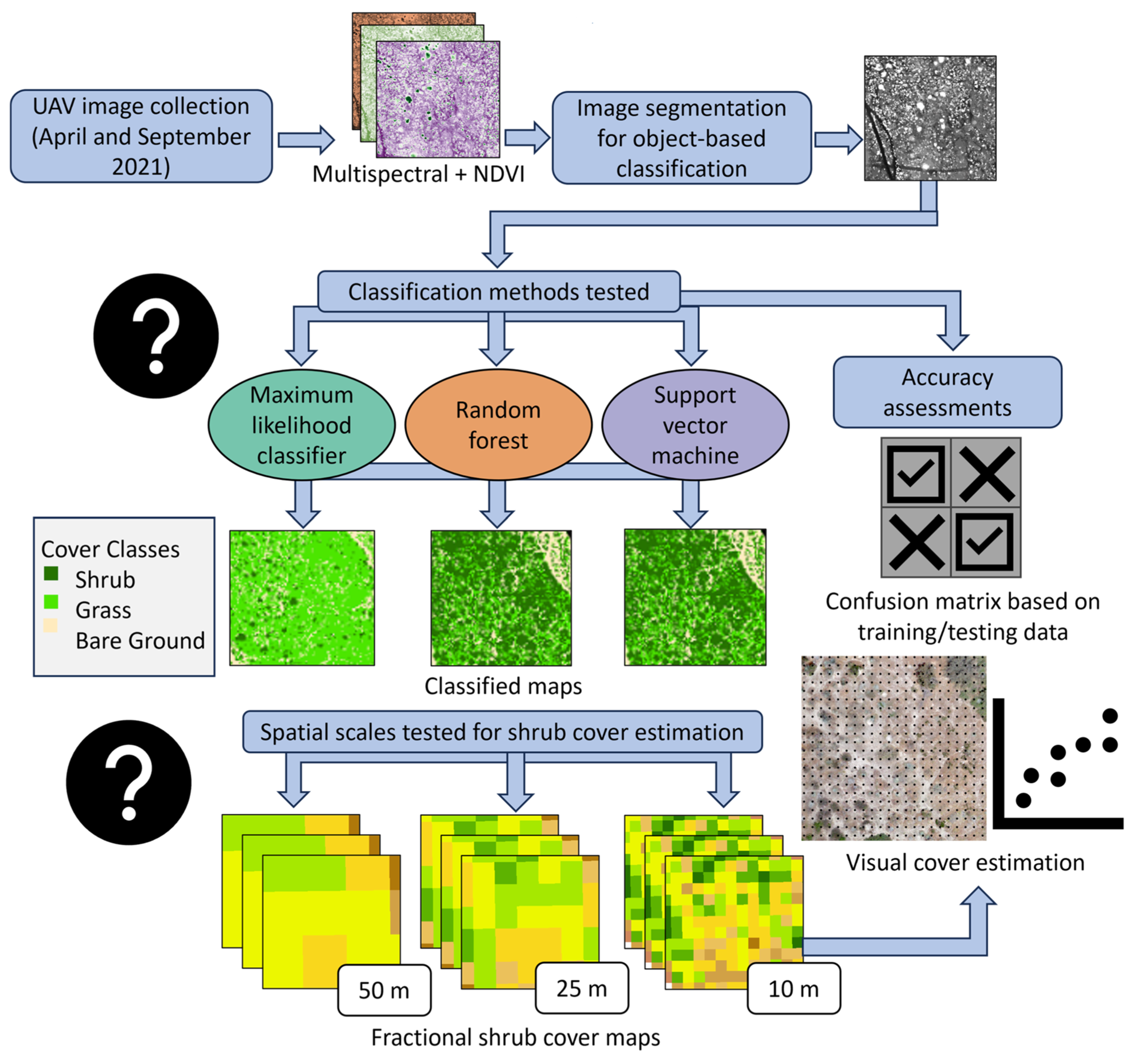
UAV-collected images were georeferenced, radiometrically corrected, and mosaicked by the vendor (Firmatek, LLC; San Antonio, TX, USA) using Pix4D software version 4.7 (Pix4D, Inc.; Denver, CO, USA). We then used Esri ArcGIS Pro version 3.0 (Esri; Redlands, CA, USA) to perform object-based image classification, fractional cover estimation, and accuracy assessment. Finally, we used R statistical software version 4.2.2 and the terra package to calculate fractional cover area estimates at different scales of aggregation [40,41]. The workflow used to classify the imagery and produce the fractional cover maps based on different grid sizes is presented in Figure 2.

2.4. Object-Based Classification

There has been strong support for object-based image analysis (OBIA) over pixel-based approaches in the context of shrub mapping [23,31,42]. For the OBIA procedure, we first performed image segmentation to group similar pixels together into segments/objects based on spectral similarity, spatial properties of resulting objects, and minimum object size (Table 2) using the Segment Mean Shift tool in Esri ArcGIS Pro version 3.0 (Esri; Redlands, CA, USA) [43,44]. Spectral detail, which controls the importance given to spectral differences between objects, was set to the maximum value (20) to achieve the best discrimination between features with similar spectral characteristics, e.g., shrub and herbaceous cover. The spatial detail and minimum segment size parameters control the importance assigned to the proximity between objects and the size of the smallest segment or object, respectively. Values for these parameters were selected by testing multiple values and visually comparing the resulting segmented images with the RGB imagery for the study area [45].
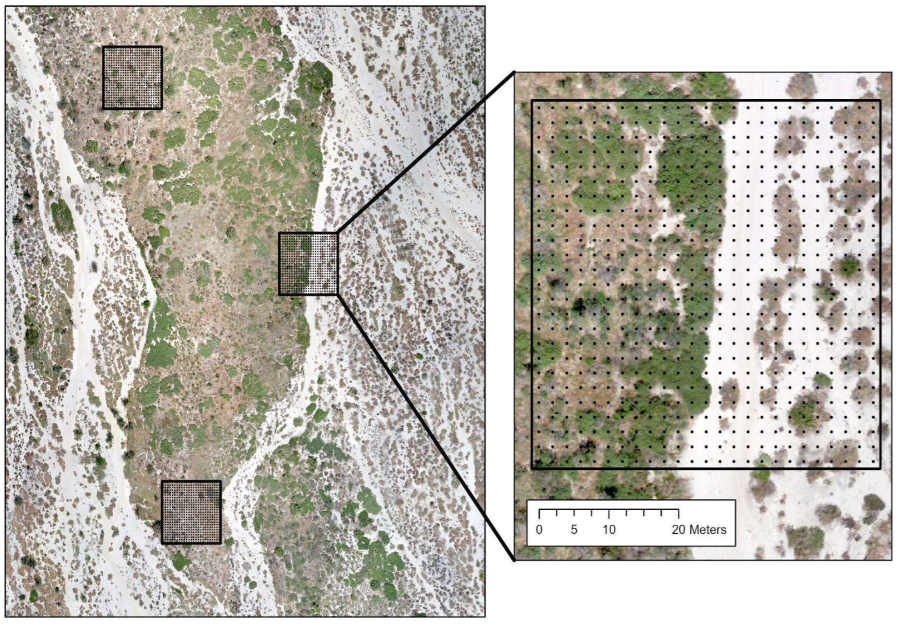
Training samples for the object-based classification procedure were collected on the segmented raster dataset, using NDVI as well as high-spatial-resolution RGB camera imagery also collected by the Parrot Sequoia+ instrument (e.g., Figure 3) as a reference for each class. Selected training samples were also validated and updated based on field observations. We selected over 200 training segments to represent each of the three classes (shrub, grass, and bare ground). The same training data were used for each of the classification algorithms (ML, RF, and SVM). The classification of the segmented image was based on the average chromaticity color, the mean digital number, standard deviation, count of pixels, compactness, and rectangularity of each segment [46,47].

2.5. Classification Algorithms

We evaluated the performance of three popular classification approaches: maximum likelihood (ML), support vector machine (SVM), and random forest (RF) implemented in ArcGIS Pro using default parameters. To evaluate the classification accuracy of each algorithm, we collected a stratified random sample of the training data and then compared the assigned classes to those produced by the classification procedure. Next, we created a confusion matrix of the producer’s accuracy (correctly classified pixels in a class divided by the number of reference pixels within that class), user’s accuracy (correctly classified pixels in a class divided by the total number of pixels that were assigned that class), overall classification accuracy (total number of correctly classified pixels divided by the total number of reference pixels), and kappa coefficient (an agreement index that accounts for agreement by chance).

2.6. Shrub Fractional Cover Estimation

We estimated and mapped shrub and non-native grass fractional cover at three scales based on the classification maps produced by each of the classification algorithms. Using the Fishnet tool in ArcGIS Pro, we created grid overlays of three different grid cell sizes: 10 × 10 m, 25 × 25 m, and 50 × 50 m. Previous research showed that spatial sampling units 25 × 25 m were most appropriate for making comparisons between coastal sage scrub communities, whereas 50 m × 50 m was most appropriate for producing cover estimates from a management perspective [31,48]. Warkentin et al. (2020) also evaluated fine-scale 10 × 10 m grid sizes to assess the areas of relatively low shrub cover, a characteristic of ecologically important pioneer phase RAFSS [23]. Percent shrub cover was then calculated within each grid cell using the Tabulate area tool. The fractional shrub cover results were rasterized and visualized using equal interval classes with 10% increments. For each classification algorithm and spatial aggregation scale, we also calculated the area of three shrub cover classes: low (10–30%), moderate (30–75%), and high (>75%). These cover classes correspond to the shrub coverage that characterizes the three RAFSS phases (pioneer, intermediate, and mature) and are, therefore, significant from a habitat management perspective. Importantly, while our analysis focuses exclusively on shrub cover, RAFSS phases are largely determined by landscape and edaphic features driven by flood dynamics and cannot be determined solely based on vegetation maps.
To assess the accuracy of fractional cover at different grid sizes, we collected reference data for fractional cover of cover for three spatial scales (10 m, 25 m, and 50 m) based on image interpretation of multispectral and true color UAV imagery of the study area using point grid sampling, an established method used to validate fractional cover estimates in shrub ecosystems [31]. We randomly selected seven 50 m plots in each management area (28 total) and divided each reference plot into 400 grid points 2.5 m apart (Figure 3). The ground cover class was recorded at each grid dot and the percent cover for each reference plot was calculated at three spatial scales: 10 m, 25 m, and 50 m. We compared fractional shrub cover collected via image interpretation (reference shrub cover) to estimates made by each classification algorithm and grid size combination (predicted shrub cover) to obtain root mean square error (RMSE), mean absolute error (MAE), and used linear regression to calculate R-squared (R2).

3. Results

3.1. Image Classification and Fractional Cover Maps

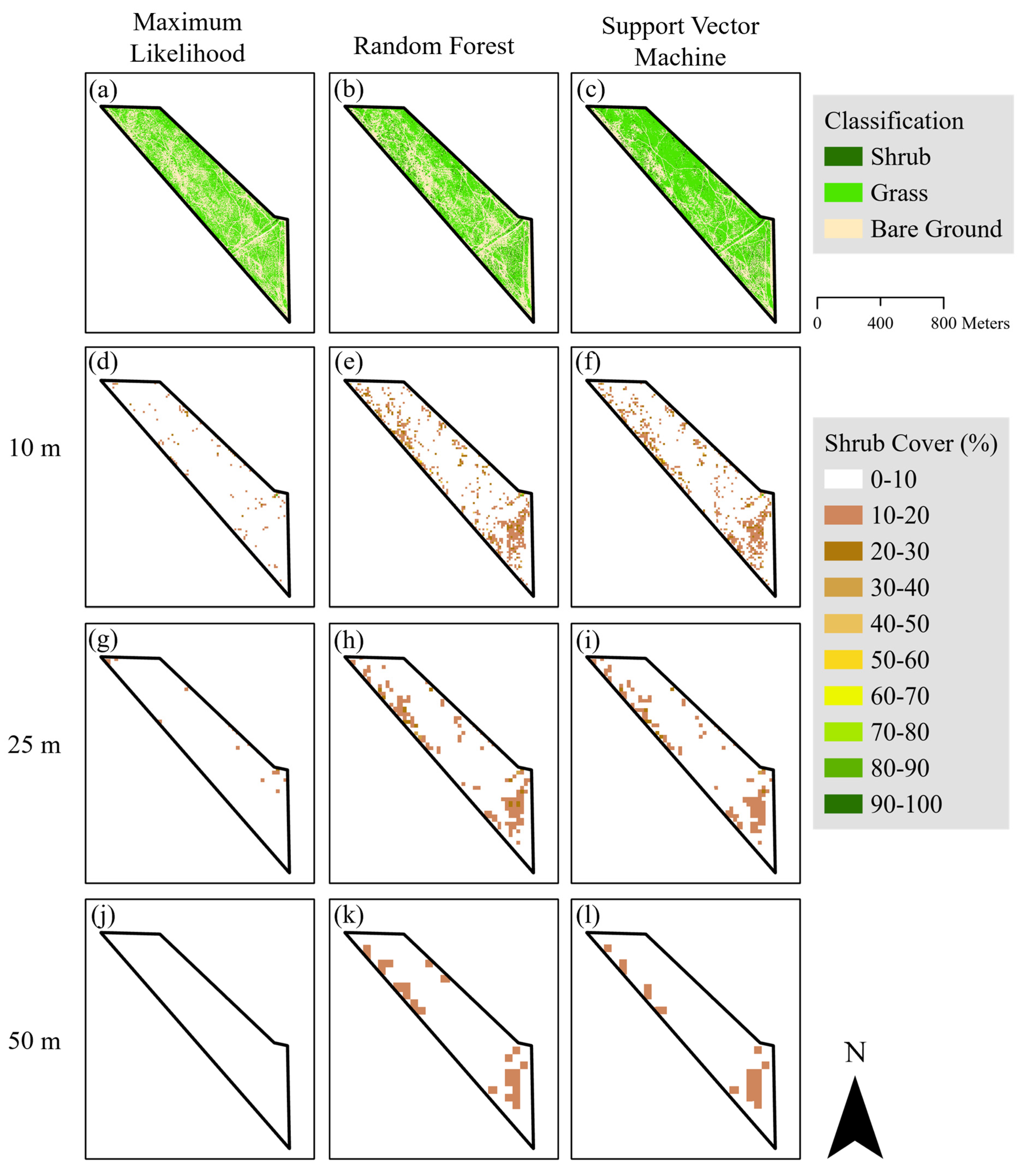
Examples of growth form and fractional shrub cover maps for area I and area NP are shown in Figure 4 and Figure 5, respectively (fractional shrub cover maps of areas H and E can be found in Figures S1 and S2). We produced fractional shrub cover maps from the growth form maps generated with spectral feature inputs to three object-based classification approaches (Figure 4a–c and Figure 5a–c). We further mapped fractional shrub cover at 10 percent intervals (Figure 4d–l and Figure 5d–l) at the three grid sizes used for estimation (10 m, 25 m, and 50 m). The classified ground cover and fractional shrub cover maps produced by the RF and SVM classifiers were quite similar in terms of the amount and spatial distribution of shrub cover predicted across each of the management areas. However, ground cover and fractional shrub cover maps produced by the ML classifier predicted lower levels of shrub cover and higher levels of grass cover than RF and SVM. This trend persisted regardless of the spatial scale used to calculate fractional shrub cover. Notably, the ML classifier identified very few areas with more than 10% shrub cover across any of the management areas. Fractional cover maps produced at the 10 m spatial scale revealed higher spatial heterogeneity in shrub cover than the maps produced at the coarser spatial scales (25 m and 50 m), at which shrub cover was more homogenous within each management area.

3.2. Accuracy Assessment

Based on internal measures of model accuracy (using a stratified random sample of the training data), the random forest had the highest classification success for all ground cover classes, as measured by overall accuracy, kappa coefficient, producer accuracy, and user accuracy (Table 3), whereas maximum likelihood had the lowest performance metrics. In terms of the most common errors, user accuracy for the grass was the lowest, indicating high commission errors in this class for all three classifiers. This pattern was mirrored by relatively low producer accuracy for the shrub class, indicating that all the classifiers struggled somewhat with assigning the class “grass” to objects that were considered “shrub” in the training data. All classifiers, including maximum likelihood, were best able to distinguish between bare ground and the vegetation classes with relatively high producer and user accuracy (≥92.80%).
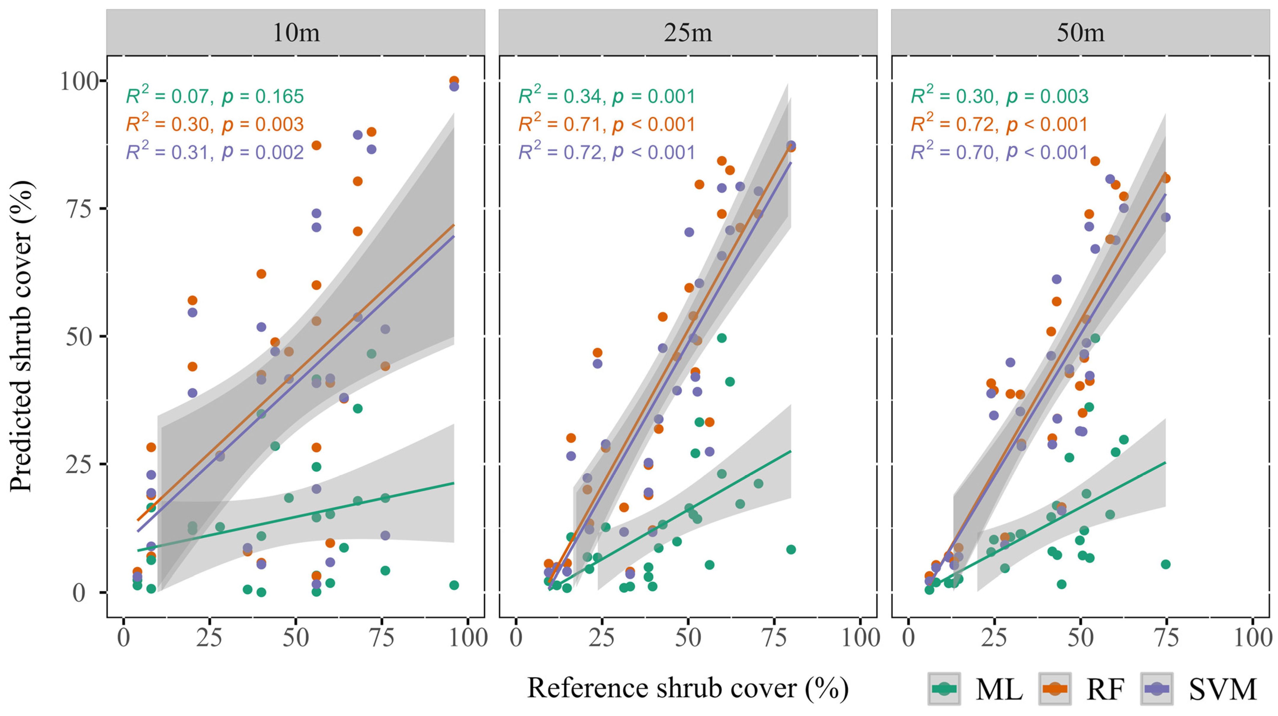
In our analysis, the 25 m and 50 m grid sizes produced the most accurate shrub cover estimates (R2 = 0.30–0.72) compared to visual interpretations of the imagery, whereas the 10 m grid size maps were the least accurate (R2 = 0.07–0.31), across the three classification algorithms (Figure 6). Maps produced by the SVM and RF algorithms produced similarly accurate estimates of fractional shrub cover, especially at grid sizes of 25 m and 50 m (Table 4: RMSE 13–15 and MAE 11–12), with R2 ranging from 0.70 to 0.72 (Figure 6). However, the ML classifier produced fractional cover estimates that were at best weakly related to the reference estimates at each of the scales of analysis (e.g., MAE 27–32), with R2 ranging from 0.07 (n.s.) to 0.34.

3.3. Fractional Shrub Cover Area Estimates

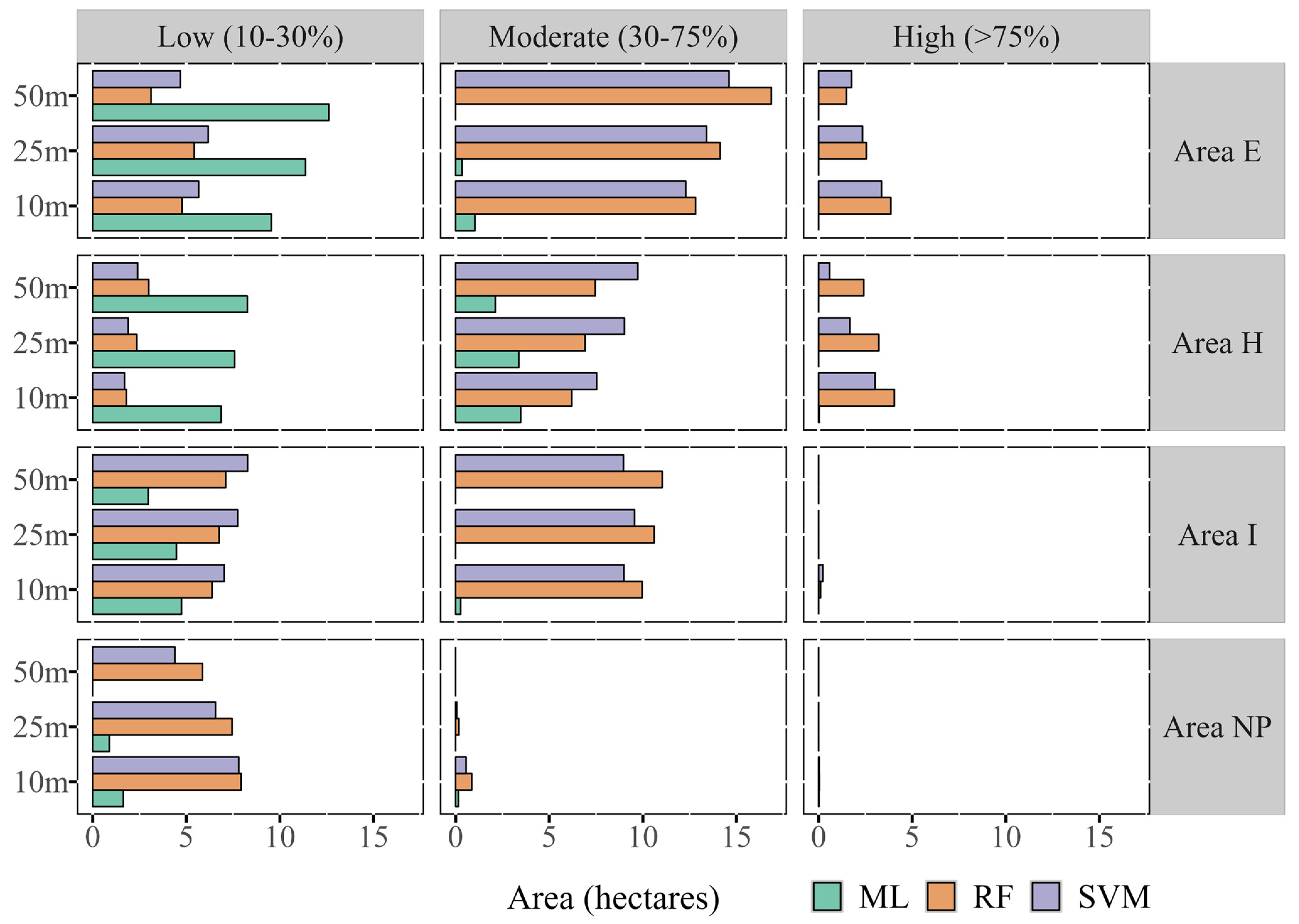
Fractional shrub cover estimates varied substantially across the management areas, classification algorithms, and grid scales included in this study (Figure 7 and Figure S3). RF and SVM produced similar estimates of shrub cover across study areas and scales of aggregation, whereas maximum likelihood produced much lower estimates (Figure S3). This resulted in greater estimates of low shrub cover and lower estimates of moderate to high shrub cover when using the maximum likelihood classifier (Figure 7). In terms of differences between management areas, we found that Area NP, located in the southeastern portion of the Cajon Creek Habitat Conservation Management Area, had the lowest fractional shrub cover by far, regardless of algorithm or grid cell size. Using the fractional shrub cover products produced by the SVM and RF algorithms, the area estimates of low shrub cover were higher in Area NP compared to estimates made by the maximum likelihood classifier, especially when using the finest grid cell size (10 m).
We also found that management areas E and H had the largest areas of high fractional shrub cover (>75%). The influence of grid cell size on area estimates for each of the shrub cover levels varied across classification algorithms and management areas. In Areas E and H, we found that fractional shrub cover maps based on the RF and SVM classifiers produced at the 10 m spatial scale predicted the largest areas of high shrub cover. Conversely, we found that the 50 m grid cell products tended to estimate the greatest expanses of moderate shrub cover (30–75%). Overall, area estimates derived from the RF and SVM map products were very similar, although the RF products tended to estimate greater moderate and high shrub coverage.

4. Discussion

A key concern in restoring and conserving arid land riparian ecosystems is the ability to assess and monitor vegetation in a cost- and time-effective manner [49]. UAV-based imagery provides the opportunity for both short- and long-term monitoring; however, transforming these data into usable products requires a substantial amount of decision-making. In this study, we evaluated the performance of three popular classifiers and different scales of analysis for mapping fractional percent shrub cover based on UAV imagery in RAFSS, a rare riparian shrub ecosystem in Southern California. We found that, using object-based image analysis, the RF and SVM classifiers were best able to accurately map fractional shrub cover based on the multispectral imagery used in this study compared to the ML classifier, which performed poorly overall. Surprisingly, we found that although fractional shrub cover maps produced at fine scales of spatial aggregation captured the widest range in shrub cover values, they tended to be less accurate than coarser scale maps. Broadly, our results support the use of UAVs in monitoring shrub cover for the purpose of conservation in RAFSS but encourage the exploration of multiple classifiers and scales of analysis when making habitat management decisions based on these products.
Understanding and quantifying vegetation cover plays an important role in assessing the need for and success of restoration and conservation efforts [50,51]. Our evaluation highlights that the choice of classification algorithm can greatly impact the accuracy of ground cover mapping and emphasizes the need for careful algorithm selection. Among the classification algorithms evaluated in this paper, we found that RF was best able to distinguish between the three ground cover classes found in the study area (shrub, grass, and bare ground), followed very closely by the SVM classifier. Although other studies have found ML classifiers to be suitable for mapping fractional vegetation cover [14], we found that this method performed quite poorly and struggled to distinguish between shrub and grass cover. Specifically, the ML classifier produced fractional cover maps that underestimated shrub cover in each of the management areas. Subsequently, fractional cover maps produced by the ML classifier showed very little to no instances of potential mature phase RAFSS (>75% shrub cover), regardless of the spatial scale used for calculating fractional shrub cover. However, based on field surveys as well as visual interpretation of the UAV imagery, we know that substantial mature phase RAFSS cover is found in two of the management areas (E and H). Erroneous results like those produced by the ML classifier could result in management incorrectly concluding that there are large areas of suitable habitat for endangered species that rely on low shrub cover or may result in management overlooking potential high shrub cover areas that could be thinned to improve suitable habitat.
We note that the confusion that led to some shrub-covered areas being classified as grass was probably in part due to the use of a single dry season image acquired when herbaceous cover is dry and not green. A time series of NDVI has been used to estimate herbaceous cover in semiarid evergreen shrubland by leveraging the intra-annual phenological differences between herbs and shrubs, albeit at moderate Landsat spatial resolution [52]. While it is well-established that large evergreen woody plants and bright soils have distinct signatures in the summer dry season [53], small semi-deciduous shrubs such as Eriogonum fasciculatum and dry, cured non-native annual grasses and forbs have similar appearances in the study area (e.g., Figure 3), apparently driving some degree of commission error in the grass category. Multitemporal imagery capturing wet and dry season (maximum and minimum herb-layer greenness) might reduce this confusion (e.g., [54]) but would also introduce additional challenges of georeferencing, radiometric correction, and differential shadowing in low-altitude UAV imagery across seasons [55]. It would also double the cost of image acquisition, which can be an important consideration in ecological monitoring and restoration [6], but this multi-temporal imagery may be warranted to help identify another key indicator, non-native cover, that would prompt restoration actions, such as herbicide application or grazing. The use of machine learning RF and SVM classifiers did yield producer accuracies of over ~90% for all considered ground cover classes; however, based only on single-season imagery. Importantly, although we found that the random forest and support vector machine classifiers were superior to the maximum likelihood algorithm in our case study, this may differ depending on the study site and ecosystem characteristics [6].
Estimating fractional vegetation cover requires decisions with respect to the size of the spatial sampling unit. While the most commonly used plot sizes for studying and managing California CSS communities are 25 × 25 m and 50 × 50 m, respectively [56,57,58], an important consideration when selecting an appropriate spatial scale for monitoring fractional shrub cover is the ability to capture changes over time—a task that may require a relatively fine spatial scale [23]. Our results demonstrate that spatial heterogeneity in estimated shrub cover was highest at the finest spatial scale included in this study (10 m) and that these map products included a greater range of shrub cover values across each of the management areas. This observation is due to the Modifiable Areal Unit Problem (MAUP), which occurs when information at broader spatial scales is based on aggregating observations that were collected at finer scales [59]. However, somewhat surprisingly, but in line with previous work in CSS [23], we found that error rates in fractional shrub cover estimates, estimated using independently collected test data, were highest at the finest spatial scale (10 m) and lowest at the coarsest (50 m)—though error levels for the 25 m scale were comparable to those found at the 50 m scale. Shrub cover estimates aggregated at these 25 and 50 m scales had low mean absolute errors, commensurate with the ecological manager’s monitoring needs, helping to target restoration actions. The fractional shrub cover estimates made using the 25 m grid provided a good balance of low error estimates and high spatial detail for restoration monitoring efforts in RAFSS, a scale that is consistent with the field sampling and fractional cover estimation scale that has been used extensively in CSS [33,56,57].

5. Conclusions

Remote sensing-based image analysis, using UAV-mounted multispectral scanners, offers great potential for monitoring habitat restoration projects [5] in support of ecological conservation. However, the uptake of these tools and methodologies has been slower in restoration ecology than in, e.g., agriculture and forestry [5]. We evaluated the potential of image classification to distinguish shrub, herbaceous, and soil ground covers and provide estimates of shrub cover needed for restoration of a rare alluvial scrub habitat in Southern California that supports several endangered species that depend on open habitats. Ground covers were classified with high accuracy based on object-based image analysis (OBIA) using the machine learning classifiers random forest and support vector machine, while maximum likelihood produced classification accuracies too low to meet restoration monitoring needs in the study area. We further tested the accuracy of shrub cover estimates aggregated to three spatial scales and found that the coarser scales test (25 and 50 m) had lower errors than 10 m scale (which had greater than 25% mean absolute error). The two coarser-scale estimates were well-calibrated with 10–12% absolute error—precise enough to be useful in restoration planning efforts in the study area aimed at maintaining different levels of shrub cover on the landscape. This study supports the use of UAV-based remote sensing for monitoring shrub cover for the purpose of restoration in this threatened habitat but shows the importance of evaluations of different classifiers and scales of analysis when making habitat management decisions based on these products. We identified areas for future research including evaluating the accuracy versus cost tradeoffs between using a single annual image versus intra-annual multitemporal images to exploit phenological differences in greenness between forbs, grasses, and shrubs.

Supplementary Materials

The following supporting information can be downloaded at: https://www.mdpi.com/article/10.3390/rs15215113/s1, Figure S1: Object-based classification for area H based on maximum likelihood, random forest, and support vector machines across the top row (a–c), with the fractional shrub cover using 10 m (d–f), 25 m (g–i) and 50 m (j–l) grid sizes.; Figure S2: Object-based classification for area E based on maximum likelihood, random forest, and support vector machines across the top row (a–c), with the fractional shrub cover using 10 m (d–f), 25 m (g–i) and 50 m (j–l) grid sizes; Figure S3: Frequency distribution for estimates of percent shrub cover in area E, area I, area M, and area NP (rows) for grid sizes 10 m, 25 m, and 50 m (columns). Results from the different classification algorithms are shown by color: maximum likelihood (ML—green), random forest (RAF—orange), and support vector machines (SVM—purple).

Author Contributions

All authors conceived and designed the study; M.M. conducted data curation and preprocessing; M.B.R. conducted image classification and data analyses presented in the manuscript and wrote the first draft; all authors contributed to writing and revising the manuscript; J.F. and L.L. acquired funding and supervised the project. All authors have read and agreed to the published version of the manuscript.

Funding

This research was supported by a research award from the Vulcan Materials Company Foundation.

Data Availability Statement

Data available upon request.

Acknowledgments

Thomas and Travis McGill (ELMT Consulting) and Sharon Lockhart (Lockhart & Associates, Inc.), acting as biological consultants and ecological restoration practitioners for Vulcan Materials Company Foundation, provided essential expert advice and access to data and unpublished reports, and were patient with our many questions during the course of this project. The photographs in Figure 1 were taken by Thomas and Travis McGill. San Diego State University, Cajon Creek, California State University, Long Beach, and UC Riverside occupy the ancestral lands of the Kumeyaay, Tongva, Acjachemen, Cahuilla, Luiseño, and Serrano peoples and we are grateful for the opportunity to conduct this research on their homelands.

Conflicts of Interest

The authors declare no conflict of interest. The funding sponsors had no role in the design of the study; in the collection, analyses, or interpretation of data; in the writing of the manuscript, and in the decision to publish the results.

References

  1. Anderson, K.; Gaston, K.J. Lightweight unmanned aerial vehicles will revolutionize spatial ecology. Front. Ecol. Environ. 2013, 11, 138–146. [Google Scholar] [CrossRef]
  2. Alvarez-Vanhard, E.; Houet, T.; Mony, C.; Lecoq, L.; Corpetti, T. Can UAVs fill the gap between in situ surveys and satellites for habitat mapping? Remote Sens. Environ. 2020, 243, 111780. [Google Scholar] [CrossRef]
  3. Michez, A.; Piégay, H.; Jonathan, L.; Claessens, H.; Lejeune, P. Mapping of riparian invasive species with supervised classification of Unmanned Aerial System (UAS) imagery. Int. J. Appl. Earth Obs. Geoinform. 2016, 44, 88–94. [Google Scholar] [CrossRef]
  4. Larrinaga, A.R.; Brotons, L. Greenness Indices from a Low-Cost UAV Imagery as Tools for Monitoring Post-Fire Forest Recovery. Drones 2019, 3, 6. [Google Scholar] [CrossRef]
  5. McKenna, P.B.; Lechner, A.M.; Hernandez Santin, L.; Phinn, S.; Erskine, P.D. Measuring and monitoring restored ecosystems: Can remote sensing be applied to the ecological recovery wheel to inform restoration success? Restor. Ecol. 2023, 31, e13724. [Google Scholar] [CrossRef]
  6. Buters, T.M.; Bateman, P.W.; Robinson, T.; Belton, D.; Dixon, K.W.; Cross, A.T. Methodological ambiguity and Inconsistency constrain unmanned aerial vehicles as a silver bullet for monitoring ecological restoration. Remote Sens. 2019, 11, 1180. [Google Scholar] [CrossRef]
  7. Phinn, S.R.; Stow, D.A.; Franklin, J.; Mertes, L.A.K.; Michaelsen, J. Remotely sensed data for ecosystem analyses: Combining hierarchy theory and scene models. Environ. Manag. 2003, 31, 429–441. [Google Scholar] [CrossRef]
  8. Kennedy, R.E.; Townsend, P.A.; Gross, J.E.; Cohen, W.B.; Bolstad, P.; Wang, Y.Q.; Adams, P. Remote sensing change detection tools for natural resource managers: Understanding concepts and tradeoffs in the design of landscape monitoring projects. Remote Sens. Environ. 2009, 113, 1382–1396. [Google Scholar] [CrossRef]
  9. Fassnacht, K.S.; Cohen, W.B.; Spies, T.A. Key Issues in making and using satellite-based maps in ecology: A primer. For. Ecol. Manag. 2006, 222, 167–181. [Google Scholar] [CrossRef]
  10. Ustin, S.L.; Middleton, E.M. Current and near-term advances in Earth observation for ecological applications. Ecol. Process. 2021, 10, 1. [Google Scholar] [CrossRef]
  11. Gann, G.D.; McDonald, T.; Walder, B.; Aronson, J.; Nelson, C.R.; Jonson, J.; Hallett, J.G.; Eisenberg, C.; Guariguata, M.R.; Liu, J.; et al. International Principles and Standards for the Practice of Ecological Restoration. Second Edition. Restor. Ecol. 2019, 27, S1–S46. [Google Scholar] [CrossRef]
  12. Bruzzone, L.; Demir, B. A review of modern approaches to classification of remote sensing data. In Land Use and Land Cover Mapping in Europe; Springer: Dordrecht, The Netherlands, 2014; pp. 127–143. [Google Scholar]
  13. Yu, L.; Liang, L.; Wang, J.; Zhao, Y.; Cheng, Q.; Hu, L.; Liu, S.; Yu, L.; Wang, X.; Zhu, P.; et al. Meta-discoveries from a synthesis of satellite-based land-cover mapping research. Int. J. Remote Sens. 2014, 35, 4573–4588. [Google Scholar] [CrossRef]
  14. Al-Ali, Z.M.; Abdullah, M.M.; Asadalla, N.B.; Gholoum, M. A comparative study of remote sensing classification methods for monitoring and assessing desert vegetation using a UAV-based multispectral sensor. Environ. Monit. Assess. 2020, 192, 389. [Google Scholar] [CrossRef] [PubMed]
  15. Adam, E.; Mutanga, O.; Odindi, J.; Abdel-Rahman, E.M. Land-use/cover classification in a heterogeneous coastal landscape using Rapid Eye imagery: Evaluating the performance of random forest and support vector machines classifiers. Int. J. Remote Sens. 2014, 35, 3440–3458. [Google Scholar] [CrossRef]
  16. Maxwell, A.E.; Warner, T.A.; Fang, F. Implementation of machine-learning classification in remote sensing: An applied review. Int. J. Remote Sens. 2018, 39, 2784–2817. [Google Scholar] [CrossRef]
  17. Mountrakis, G.; Im, J.; Ogole, C. Support vector machines in remote sensing: A review. ISPRS J. Photogramm. Remote Sens. 2011, 66, 247–259. [Google Scholar] [CrossRef]
  18. Foody, G.M.; Mathur, A. The use of small training sets containing mixed pixels for accurate hard image classification: Training on mixed spectral responses for classification by a SVM. Remote Sens. Environ. 2006, 103, 179–189. [Google Scholar] [CrossRef]
  19. Breiman, L. Random Forests. Mach. Learn. 2001, 45, 5–32. [Google Scholar] [CrossRef]
  20. Sheykhmousa, M.; Mahdianpari, M.; Ghanbari, H.; Mohammadimanesh, F.; Ghamisi, P.; Homayouni, S. Support vector machine versus random forest for remote sensing image classification: A meta-analysis and systematic review. IEEE J. Sel. Top. Appl. Earth Obs. Remote Sens. 2020, 13, 6308–6325. [Google Scholar] [CrossRef]
  21. Chu, D. Fractional Vegetation Cover. In Remote Sensing of Land Use and Land Cover in Mountain Region, 2nd ed.; Liang, S., Wang, J., Eds.; Academic Press: Cambridge, MA, USA, 2020; pp. 477–510. ISBN 978-0-12-815826-5. [Google Scholar]
  22. Herrick, J.E.; Schuman, G.E.; Rango, A. Monitoring ecological processes for restoration projects. J. Nat. Conserv. 2006, 14, 161–171. [Google Scholar] [CrossRef]
  23. Warkentin, K.; Stow, D.; Uyeda, K.; O’Leary, J.; Lambert, J.; Loerch, A.; Coulter, L. Shrub fractional cover estimation and mapping of San Clemente Island shrubland based on airborne multispectral imagery and lidar data. Remote Sens. 2020, 12, 3608. [Google Scholar] [CrossRef]
  24. Wiens, J.A. Spatial scaling in ecology. Funct. Ecol. 1989, 3, 385–397. [Google Scholar] [CrossRef]
  25. Lindenmayer, D.; Hobbs, R.J.; Montague-Drake, R.; Alexandra, J.; Bennett, A.; Burgman, M.; Cale, P.; Calhoun, A.; Cramer, V.; Cullen, P.; et al. A checklist for ecological management of landscapes for conservation. Ecol. Lett. 2008, 11, 78–91. [Google Scholar] [CrossRef]
  26. Mitrovich, L.; Lockhart, S.; Sprague, D.W. Case Study: Cajon Creek Habitat Conservation Management Area. Tran. West. Sect. Wild. Soc. 1999, 35, 57–62. [Google Scholar]
  27. Hanes, T.L.; Friesen, R.D.; Keane, K. Alluvial scrub vegetation in coastal southern California. In California Riparian System Conference; USDA Forest Service General Technical Report PSW-110; USDA: Davis, CA, USA, 1989; pp. 187–193. [Google Scholar]
  28. Chock, R.Y.; McCullough Hennessy, S.; Wang, T.B.; Gray, E.; Shier, D.M. A multi-model approach to guide habitat conservation and restoration for the endangered San Bernardino kangaroo rat. Global Ecol. Conserv. 2020, 21, e00881. [Google Scholar] [CrossRef]
  29. Burk, J.H.; Eugene Jones, C.; Ryan, W.A.; Wheeler, J.A. Floodplain vegetation and soils along the upper Santa Ana River, San Bernardino County, California. Madroño 2007, 54, 126–137. [Google Scholar] [CrossRef]
  30. Cleland, E.E.; Funk, J.L.; Allen, E.B. Coastal sage scrub. In Ecosystems of California; Mooney, H.A., Zavaleta, E.S., Eds.; University of California Press: Oakland, CA, USA, 2016; pp. 429–448. [Google Scholar]
  31. Hamada, Y.; Stow, D.A.; Roberts, D.A. Estimating life-form cover fractions in California sage scrub communities using multispectral remote sensing. Remote Sens. Environ. 2011, 115, 3056–3068. [Google Scholar] [CrossRef]
  32. Lippitt, C.L.; Stow, D.A.; Roberts, D.A.; Coulter, L.L. Multidate MESMA for Monitoring Vegetation Growth Forms in Southern California Shrublands. Int. J. Remote Sens. 2018, 39, 655–683. [Google Scholar] [CrossRef]
  33. Hamada, Y.; Stow, D.A.; Franklin, J. Quantifying biological integrity of California sage scrub communities using plant life-form cover. J. Mediterr. Ecol. 2009, 10, 19–32. [Google Scholar]
  34. Martin, L.J.; Blossey, B.; Ellis, E. Mapping where ecologists work: Biases in the global distribution of terrestrial ecological observations. Front. Ecol. Environ. 2012, 10, 195–201. [Google Scholar] [CrossRef]
  35. Murphy, G.E.P.; Romanuk, T.N. Data gaps in anthropogenically driven local-scale species richness change studies across the Earth’s terrestrial biomes. Ecol. Evol. 2016, 6, 2938–2947. [Google Scholar] [CrossRef] [PubMed]
  36. Burk, J.H.; Jones, C.E.; Wheeler, J.; DeSimone, S. The Ecology of Eriastrum densifolium sanctorum (Milliken) Mason; Department of the Army, The Corps of Engineers (COE): Los Angeles, CA, USA, 1988. [Google Scholar]
  37. Hernandez, R.R.; Sandquist, D.R. A dam in the drylands: Soil geomorphic treatments facilitate recruitment of the endangered Santa Ana River woolly star. Ecosphere 2019, 10, e02621. [Google Scholar] [CrossRef]
  38. Smith, R.L. The Alluvial Scrub Vegetation of the San Gabriel River Floodplain; California State University: Fullerton, CA, USA, 1978. [Google Scholar]
  39. Tucker, C.J. Red and photographic infrared linear combinations for monitoring vegetation. Remote Sens. Environ. 1979, 8, 127–150. [Google Scholar] [CrossRef]
  40. Hijmans, R.J.; Bivand, R.; Forner, K.; Ooms, J.; Pebesma, E.; Sumner, M.D. Package “terra.”; Maintainer: Vienna, Austria, 2022. [Google Scholar]
  41. R Core Team R: A Language and Environment for Statistical Computing; R Foundation for Statistical Computing: Vienna, Austria, 2023.
  42. Laliberte, A.S.; Browning, D.M.; Herrick, J.E.; Gronemeyer, P. Hierarchical object-based classification of ultra-high-resolution Digital Mapping Camera (DMC) imagery for rangeland mapping and assessment. J. Spat. Sci. 2010, 55, 101–115. [Google Scholar] [CrossRef]
  43. Comaniciu, D.; Meer, P. Mean shift: A robust approach toward feature space analysis. IEEE Trans. Pattern Anal. Mach. Intell. 2002, 24, 603–619. [Google Scholar] [CrossRef]
  44. ArcGIS Desktop Help Segment Mean Shift. Available online: https://pro.arcgis.com/en/pro-app/latest/help/analysis/raster-functions/segment-mean-shift-function.htm (accessed on 25 August 2023).
  45. Collins, J.; Dronova, I. Urban landscape change analysis using local climate zones and object-based classification in the Salt Lake metro region, Utah, USA. Remote Sens. 2019, 11, 1615. [Google Scholar] [CrossRef]
  46. Darwish, A.; Leukert, K.; Reinhardt, W. Image Segmentation for the Purpose of Object-based Classification. In Proceedings of the 2003 IEEE International Conference on Geoscience and Remote Sensing Symposium, IGARSS’03, Toulouse, France, 21–25 July 2003; IEEE International: Piscataway, NJ, USA, 2003; pp. 2039–2041. [Google Scholar]
  47. ArcGIS Desktop Help Classify. Available online: https://pro.arcgis.com/en/pro-app/latest/help/analysis/image-analyst/classify.htm (accessed on 25 August 2023).
  48. Hamada, Y.; Stow, D.A.; Roberts, D.A.; Franklin, J.; Kyriakidis, P.C. Assessing and monitoring semi-arid shrublands using object-based image analysis and multiple endmember spectral mixture analysis. Environ. Monit. Assess. 2013, 185, 3173–3190. [Google Scholar] [CrossRef]
  49. Gómez-Sapiens, M.; Schlatter, K.J.; Meléndez, Á.; Hernández-López, D.; Salazar, H.; Kendy, E.; Flessa, K.W. Improving the efficiency and accuracy of evaluating aridland riparian habitat restoration Using unmanned aerial vehicles. Remote Sens. Ecol. Conserv. 2021, 7, 488–503. [Google Scholar] [CrossRef]
  50. Corrêa, R.S.; Balduíno, A.P.d.C.; Teza, C.T.V.; Baptista, G.M.d.M. Vegetation cover development resulting from different restoration approaches of exploited mines. Floresta Ambient. 2018, 25, e20171116. [Google Scholar] [CrossRef]
  51. Dale, J.; Burnside, N.G.; Hill-Butler, C.; Berg, M.J.; Strong, C.J.; Burgess, H.M. The use of unmanned aerial vehicles to determine differences in vegetation cover: A tool for monitoring coastal wetland restoration schemes. Remote Sens. 2020, 12, 4022. [Google Scholar] [CrossRef]
  52. Park, I.W.; Hooper, J.; Flegal, J.M.; Jenerette, G.D. Impacts of climate, disturbance and topography on distribution of herbaceous cover in Southern California chaparral: Insights from a remote-sensing method. Divers. Distrib. 2018, 24, 497–508. [Google Scholar] [CrossRef]
  53. Franklin, J.; Davis, F.W.; Lefebvre, P. Thematic mapper analysis of tree cover in semiarid woodlands using a model of canopy shadowing. Remote Sens. Environ. 1991, 36, 189–202. [Google Scholar] [CrossRef]
  54. Schmidt, T.; Schuster, C.; Kleinschmit, B.; Förster, M. Evaluating an intra-annual time series for grassland classification—How many acquisitions and what seasonal origin are optimal? IEEE J. Sel. Top. Appl. Earth Obs. Remote Sens. 2014, 7, 3428–3439. [Google Scholar] [CrossRef]
  55. Delavarpour, N.; Koparan, C.; Nowatzki, J.; Bajwa, S.; Sun, X. A Technical study on UAV characteristics for precision agriculture applications and associated practical challenges. Remote Sens. 2021, 13, 1204. [Google Scholar] [CrossRef]
  56. Malanson, G.P. Fire history and patterns of Venturan subassociations of Californian coastal sage scrub. Vegetatio 1984, 57, 121–128. [Google Scholar] [CrossRef]
  57. Westman, W.E. Diversity Relations and Succession in Californian Coastal Sage Scrub. Ecology 1981, 62, 170–184. [Google Scholar] [CrossRef]
  58. Diffendorfer, J.E.; Fleming, G.M.; Duggan, J.M.; Chapman, R.E.; Rahn, M.E.; Mitrovich, M.J.; Fisher, R.N. Developing Terrestrial, Multi-Taxon Indices of Biological Integrity: An Example from Coastal Sage Scrub. Biol. Conserv. 2007, 140, 130–141. [Google Scholar] [CrossRef]
  59. Dark, S.J.; Bram, D. The Modifiable Areal Unit Problem (MAUP) in Physical Geography. Prog. Phys. Geogr. 2007, 31, 471–479. [Google Scholar] [CrossRef]
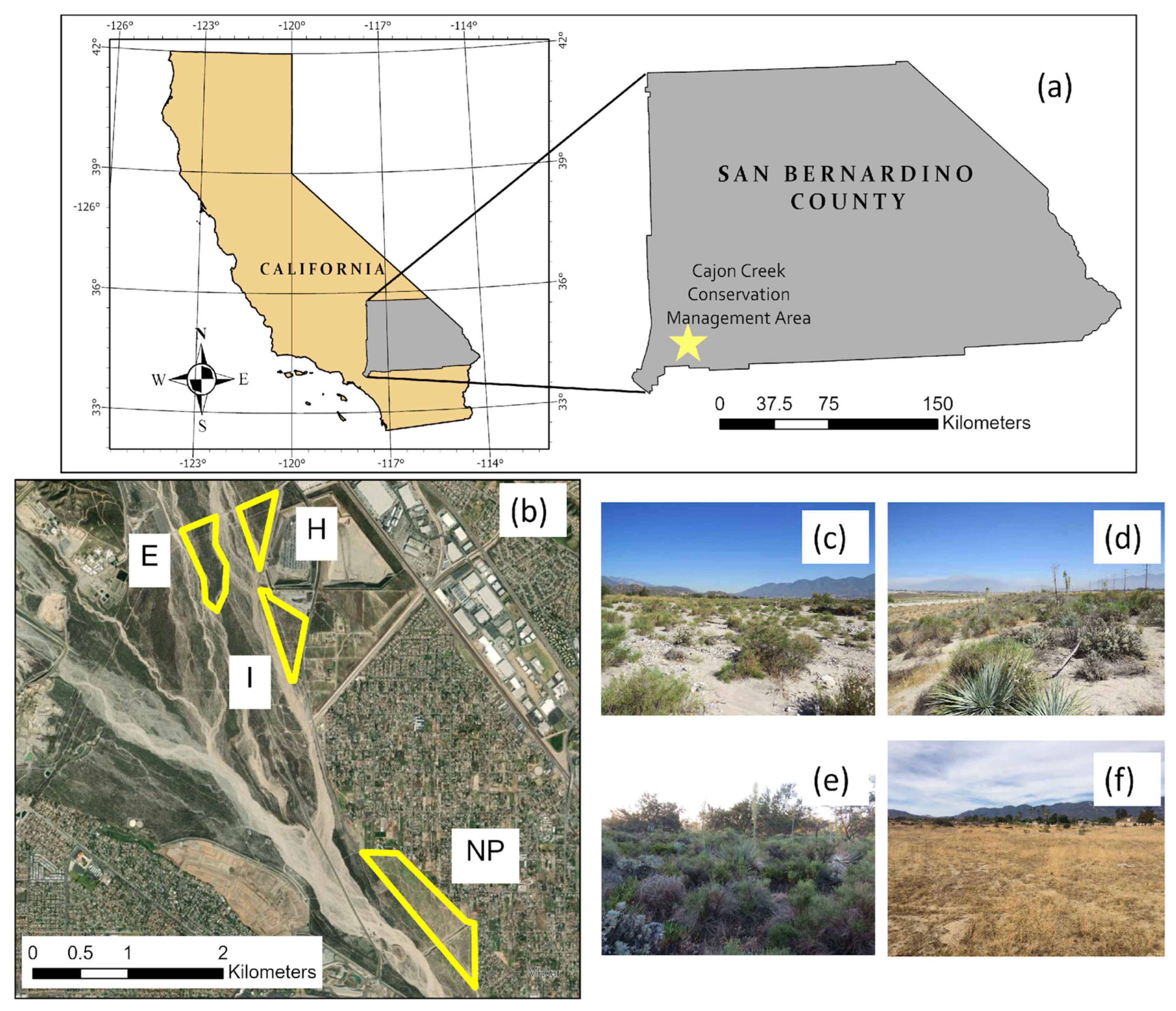
Figure 1. Maps and field photos of the study area. Map showing the location of the Cajon Creek Conservation Management Area in San Bernardino County and the state of California (a). Locations of the four habitat restoration sites within the Cajon Creek Conservation Management Area outlined in yellow on the aerial image map (Source: Esri, Maxar, Earthstar Geographics, and the GIS User Community): E, H, I, and NP (b). Photographs of pioneer Riversidean Alluvial Fan Sage Scrub (RAFSS) (c), intermediate RAFSS (d), mature RAFSS (e), and non-native herbaceous cover (f).
Remotesensing 15 05113 g001
Figure 2. Data and methods workflow for comparing classification algorithms and spatial scales for assessing key vegetation monitoring indicators. Question marks indicate the two research objectives: compare the accuracy of three supervised classification approaches to map cover and compare the accuracy of three grid-cell sizes for estimating fractional shrub cover.
Remotesensing 15 05113 g002
Figure 3. Sampling grid overlaid on RGB imagery collected in April 2021 used for calculating the percent cover (image interpretation). Grid points are 2.5 m apart in 50 × 50 m plots.
Remotesensing 15 05113 g003
Figure 4. Object-based classification for area I based on maximum likelihood, random forest, and support vector machine across the top row (ac), with the fractional shrub cover derived using 10 m (df), 25 m (gi), and 50 m (jl) grid sizes below.
Remotesensing 15 05113 g004
Figure 5. Object-based classification for area NP based on maximum likelihood, random forest, and support vector machine across the top row (ac), with the fractional shrub cover derived using 10 m (df), 25 m (gi), and 50 m (jl) grid sizes below.
Remotesensing 15 05113 g005
Figure 6. Scatter plots and linear trend lines of reference shrub cover (%) based on reference data from visual image estimation (Figure 3) and predicted shrub cover (%) estimated by each of the classification algorithms shown in different colors (ML = maximum likelihood; RF = random forest; SVM = support vector machine) and grid size combinations. Shaded gray areas indicate 95% confidence intervals.
Remotesensing 15 05113 g006
Figure 7. Area estimates (hectares) for three levels of fractional shrub cover (columns) in the four management areas (rows) based on the classification algorithms shown in different colors (ML = maximum likelihood; RF = random forest; SVM = support vector machine) and grid cell size combinations.
Remotesensing 15 05113 g007
Table 1. Technical specifications of UAV imagery used in classification and visual interpretation.
ParametersSpecifications
Date of image acquisitionApril 2021 (RGB Composite)
September 2021 (Multispectral)
Sensor typeMultispectral (Parrot Sequoia+)
Spectral bands|Wavelength|BandwidthGreen: 550 nm ± 40 nm
Red: 660 nm ± 40 nm
Red-Edge: 735 nm ± 10 nm
Near-Infrared: 790 nm ± 40 nm
Spatial resolution0.14 m
Field of viewHorizontal: 62° (Multispectral); 64° (RGB)
Vertical: 49° (Multispectral); 50° (RGB)
Diagonal: 74° (Multispectral and RGB)
Flying height400 feet (121.92 m) above ground level
Table 2. Parameters of the segmentation process carried out in ArcGIS Pro for the OBIA classification.
ParameterDescriptionInput Data
Input raster bandsRaster data used for segmentationGreen
Red edge
NDVI (NIR − Red)/(NIR + Red)
Spectral DetailControls the level of importance given to the spectral differences of objects. Values range from 1 to 20. Smaller values create spectrally smooth outputs, while higher spectral detail allows for greater discrimination between objects with similar spectral characteristics.20
Spatial DetailControls the level of importance given to the proximity between objects. Values range from 1 to 20, where higher values allow for smaller, more clustered objects.15
Minimum
Segment Size
Controls the size of the smallest segment/object in pixels.20
Table 3. Accuracy assessment of vegetation cover classes for three classification algorithms (maximum likelihood, random forest, and support vector machine).
Classification AlgorithmClassesOverall Accuracy (%)Kappa CoefficientProducer Accuracy (%)User Accuracy (%)
Maximum LikelihoodBare ground88.000.6892.8099.20
Shrub 50.00100
Grass 92.6840.00
Random ForestBare ground97.600.9398.00100
Shrub 94.6498.15
Grass 97.5678.43
Support Vector MachineBare ground96.400.8997.5299.75
Shrub 89.2998.04
Grass 95.1270.90
Table 4. Root mean square error (RMSE) and mean absolute error (MAE) values for the fractional shrub cover estimates made by each of the classification algorithms and grid sizes.
10 m25 m50 m
Classification AlgorithmRMSEMAERMSEMAERMSEMAE
Maximum Likelihood39.7431.8932.5928.8630.5326.66
Random Forest26.0019.1914.9912.2713.3011.17
Support Vector Machine25.8719.6114.5512.2412.8510.80
Disclaimer/Publisher’s Note: The statements, opinions and data contained in all publications are solely those of the individual author(s) and contributor(s) and not of MDPI and/or the editor(s). MDPI and/or the editor(s) disclaim responsibility for any injury to people or property resulting from any ideas, methods, instructions or products referred to in the content.