
A Method for Convergent Deformation Analysis of a Shield Tunnel Incorporating B-Spline Fitting and ICP Alignment


Abstract
:1. Introduction
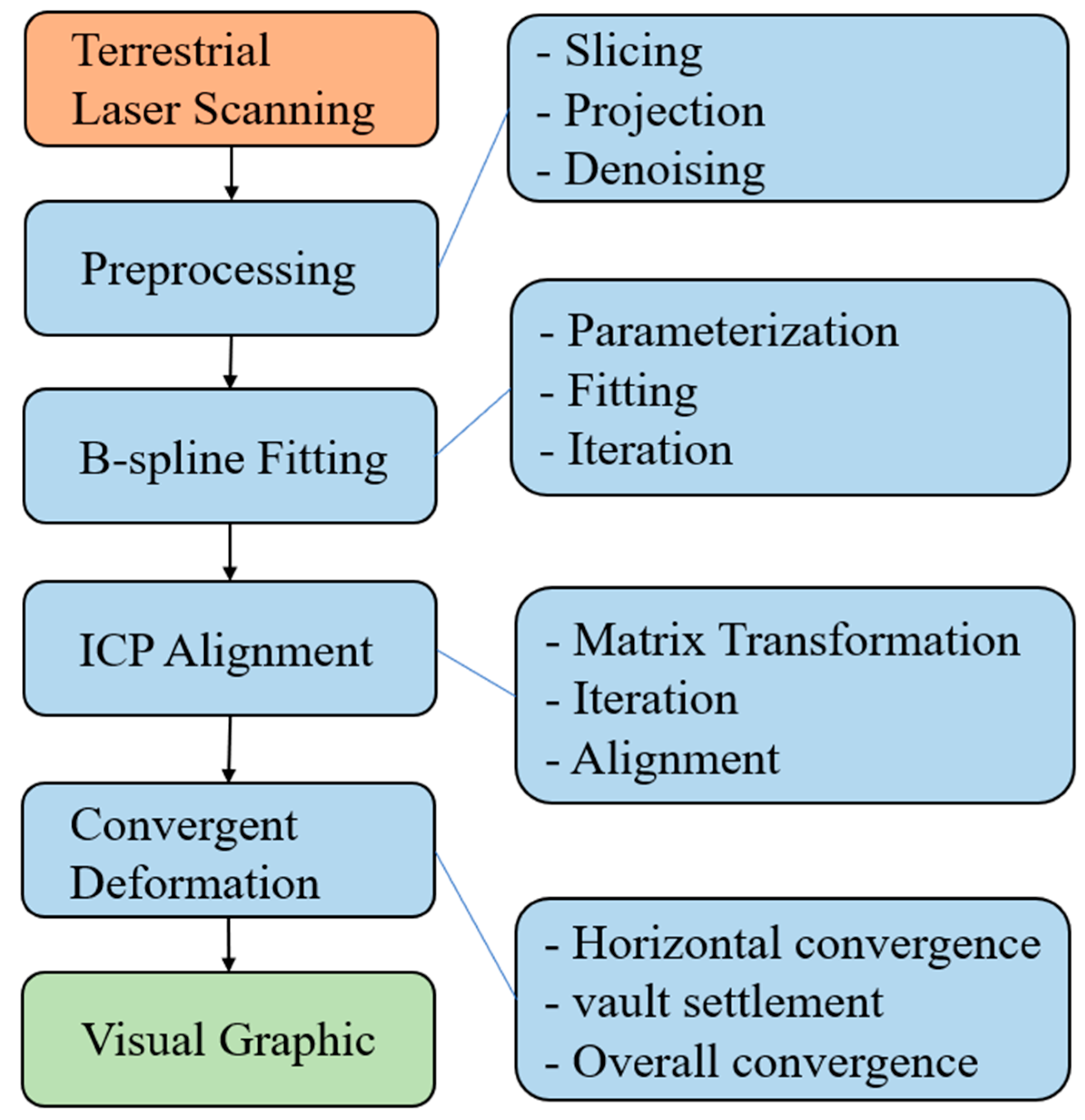
2. Methods
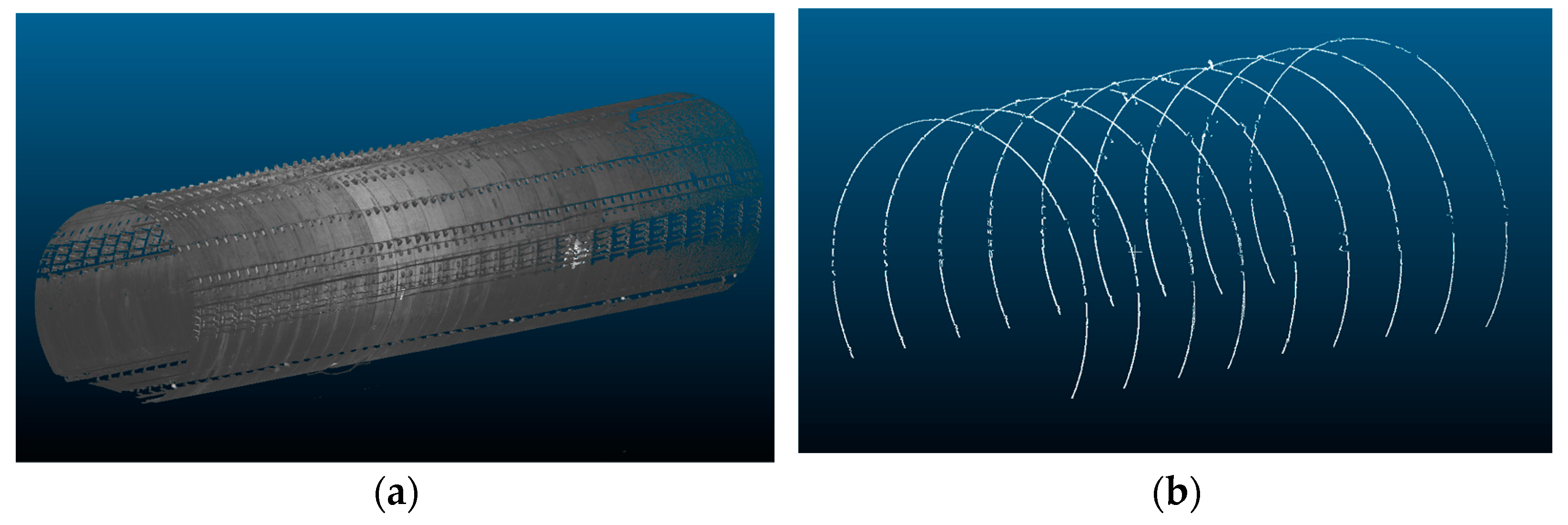
2.1. Pre-Processing
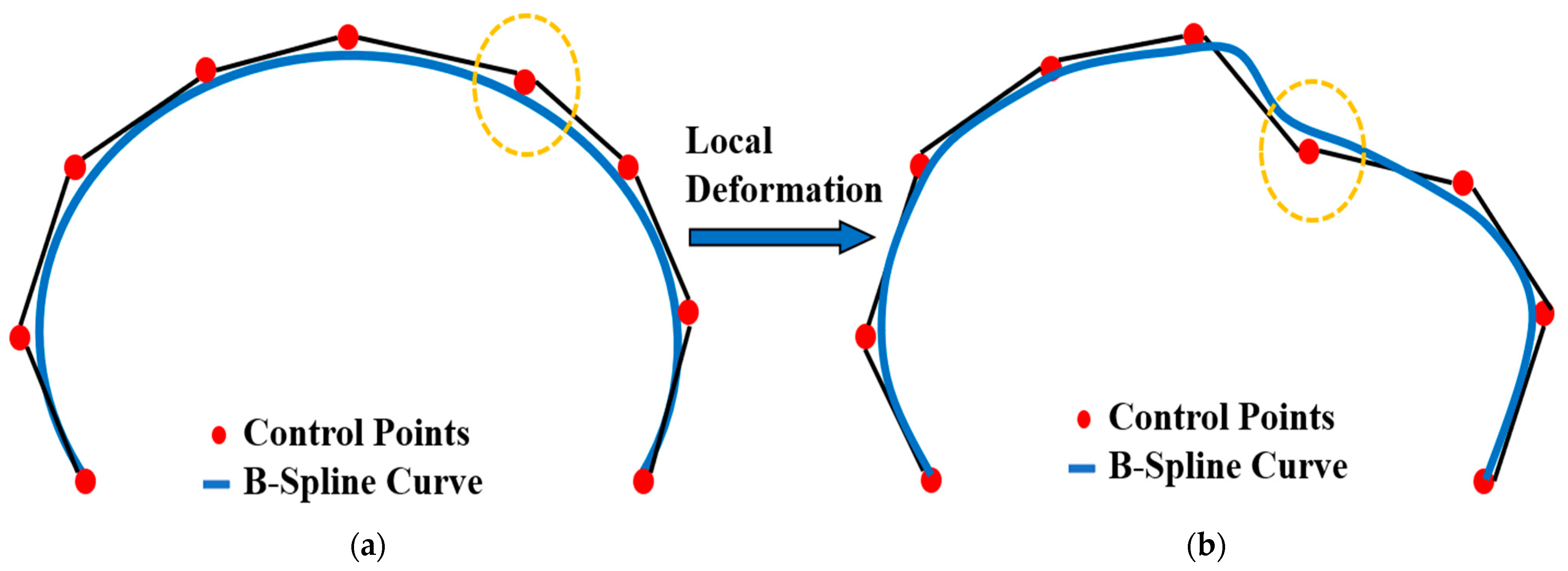
2.2. B-Spline Curve Fitting
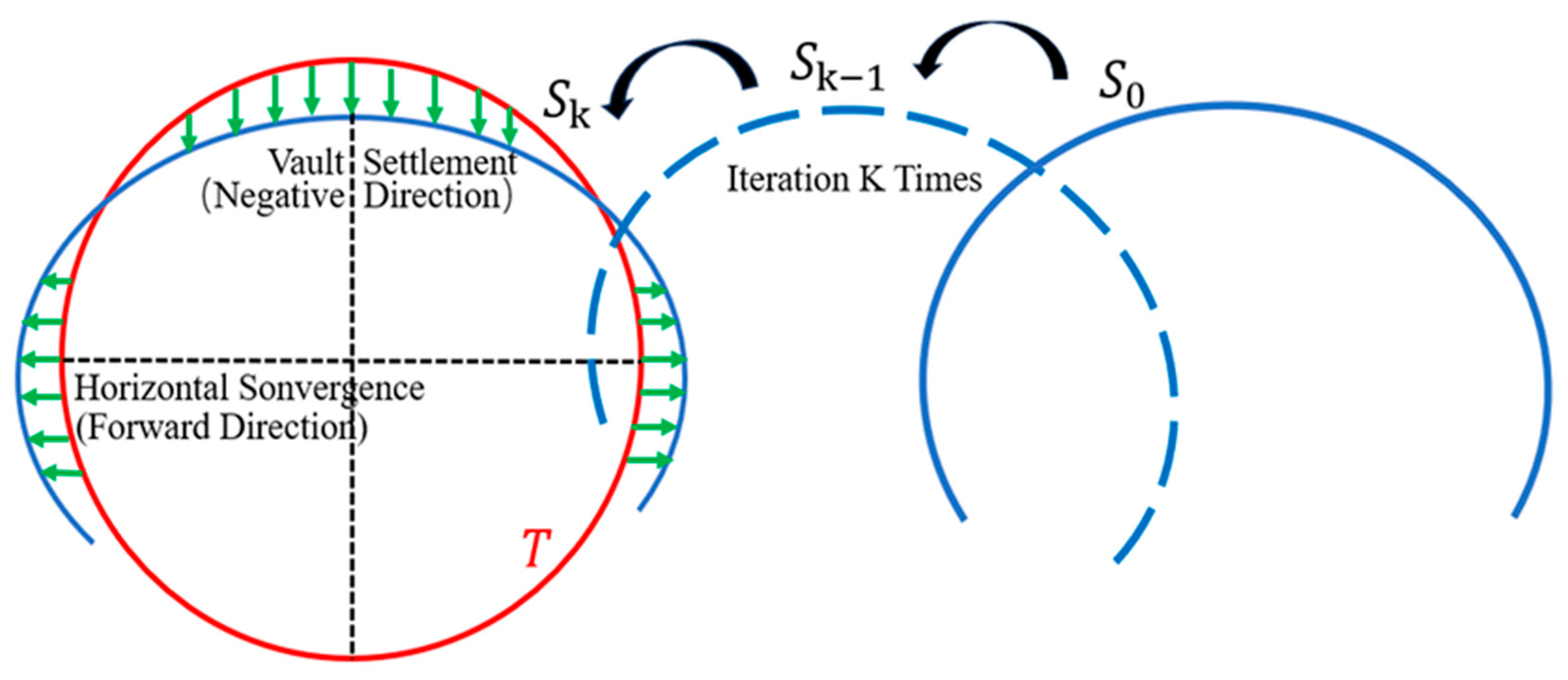
2.3. ICP Alignment
- 1.
- Calculate and to minimize according to Equations (4)–(6).
- 2.
- Update according to Equation (7). Third item.
- 3.
- Replace with in Equation (4).
- 4.
- Determine the correspondence between the final S and T. Calculate the convergent deformation at each point of the tunnel cross-section according to the Euclidean distance Equation (8). Calculate the overall convergent deformation of the tunnel cross-section according to the root mean square Equation (9).
- 5.
- Repeat steps 1–4 and the iteration stops when the objective is satisfied according to Equation (9).
2.4. Comparison of Method
3. Results
3.1. Data Selection
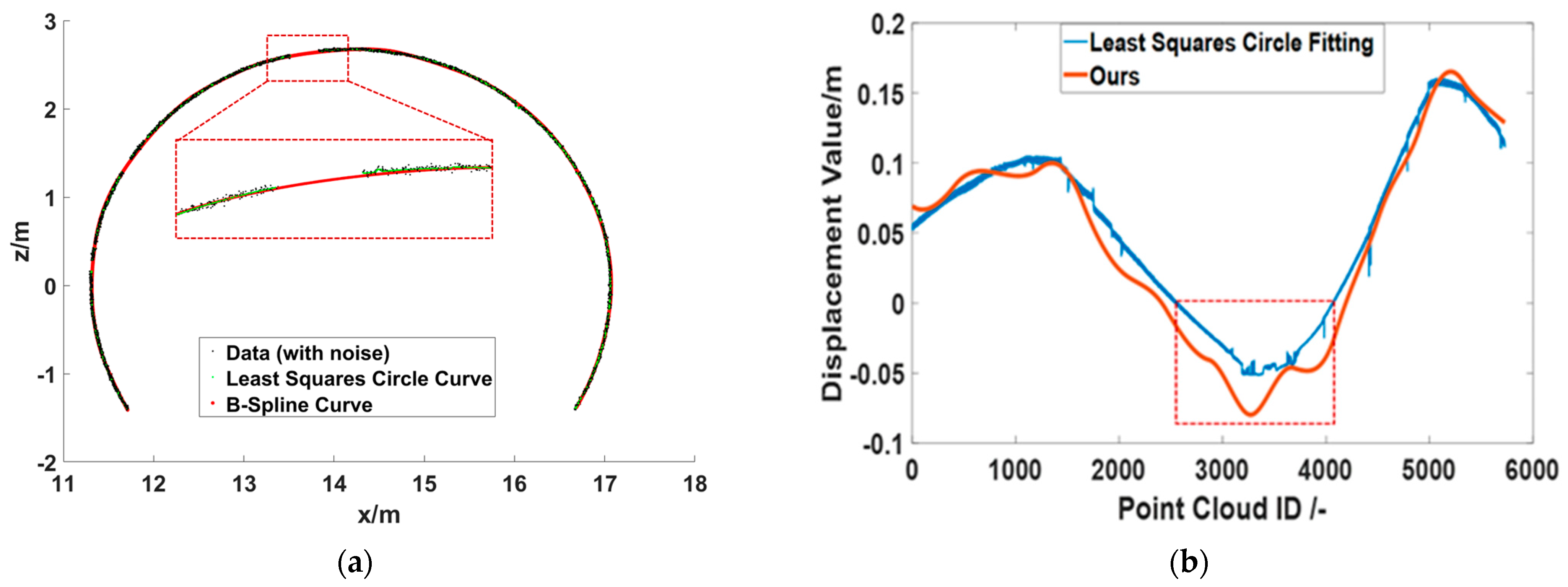
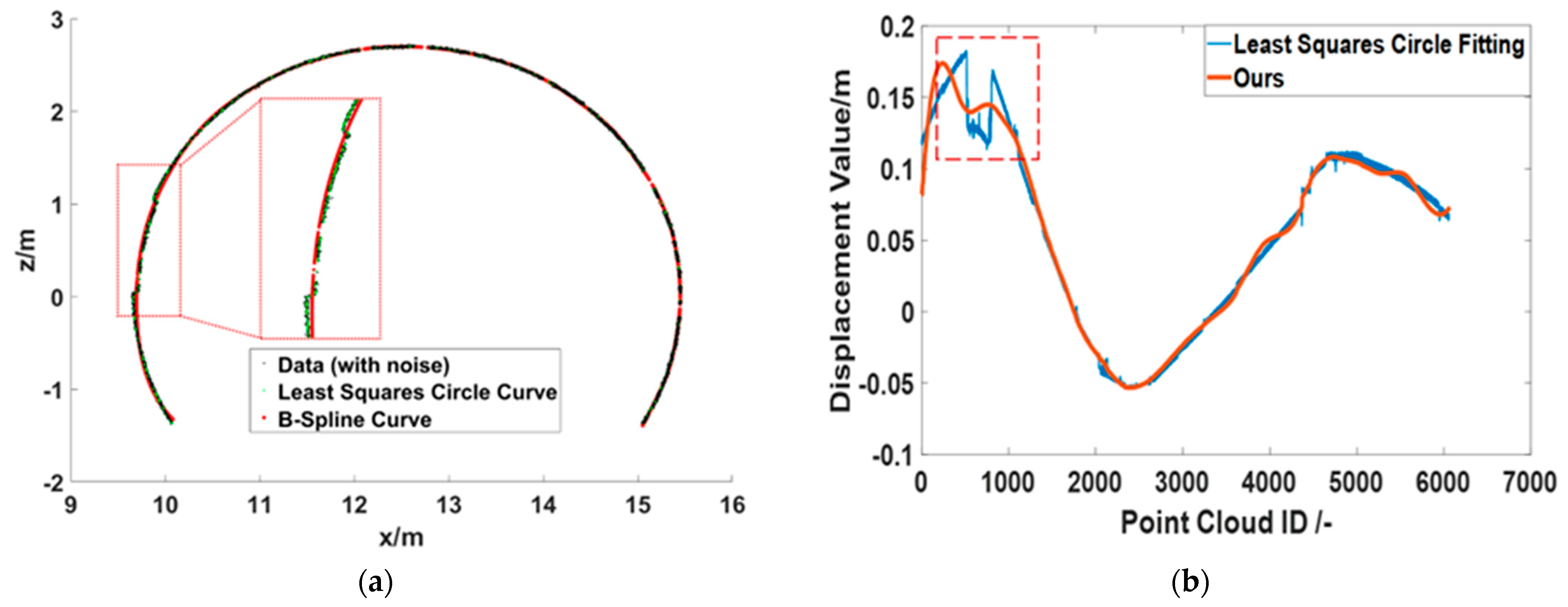
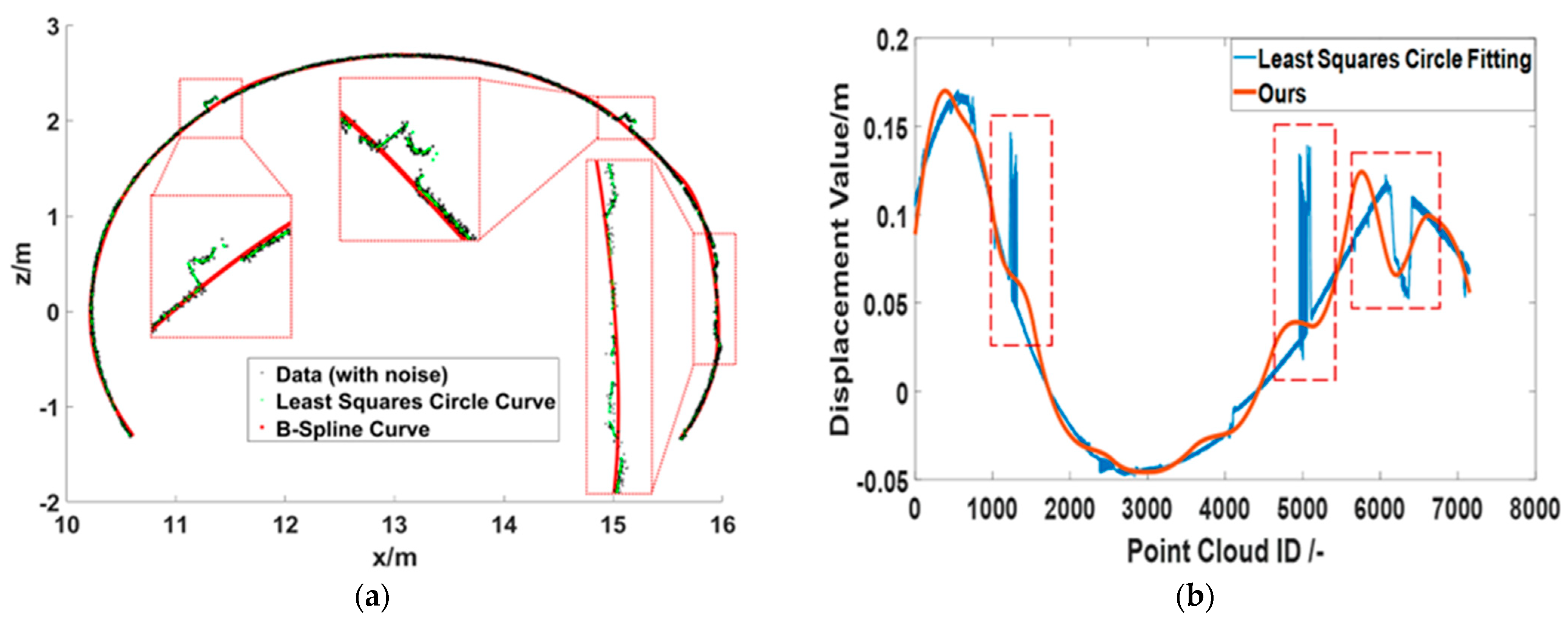
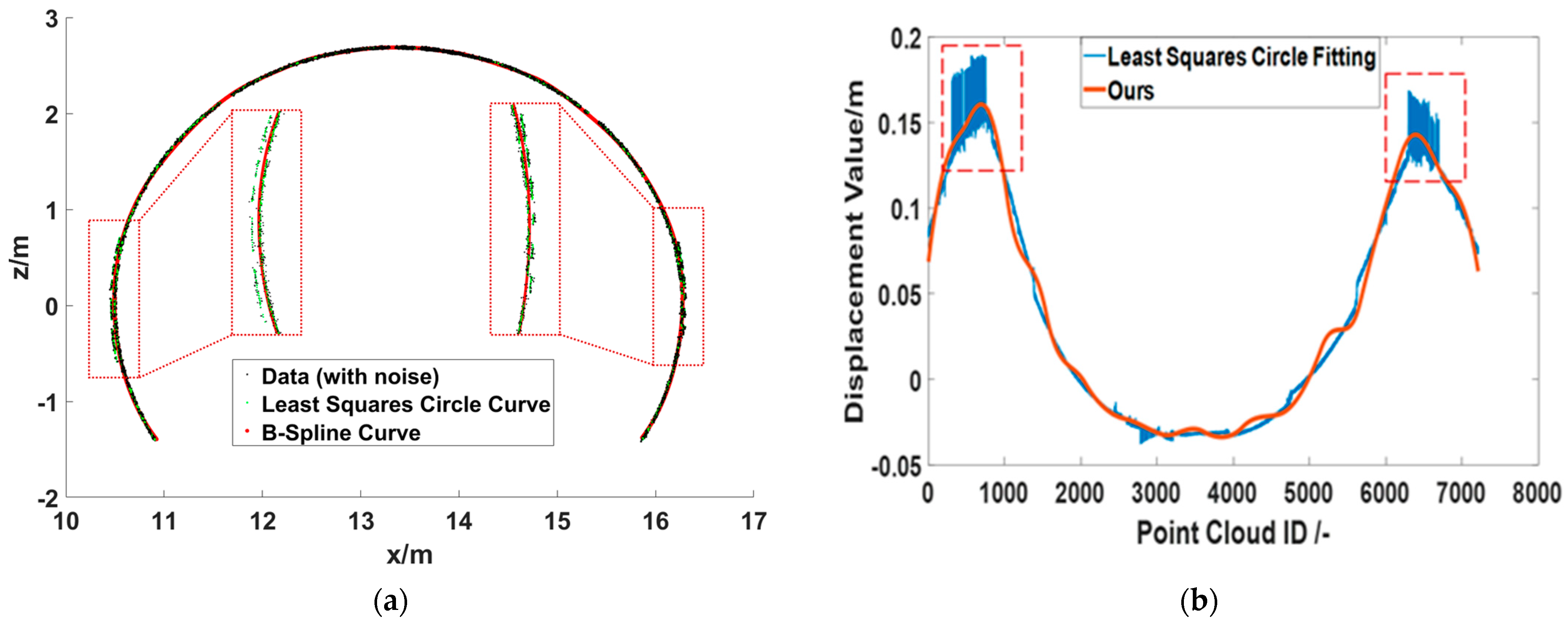
3.2. Experimental Results
3.3. Deformation Visualization
4. Discussion
5. Conclusions
- A high-precision tunnel deformation monitoring method incorporating B-spline fitting and ICP alignment is proposed to monitor horizontal convergence, vault settlement and circumferential convergence with high accuracy.
- Compared with the circle fitting algorithm, our method can automatically compensate for the missing point clouds, is not affected by the point clouds of the lining appendages inside and outside the tunnel, and is more sensitive concerning the feedback of local deformation.
- The calculation of the difference between the radial distance and the design radius of a tunnel is transformed into a curve transformation that iterates over the nearest neighbors and calculates the difference in the distance between the corresponding points; therefore, our method can be applied to a variety of tunnel shapes.
Author Contributions
Funding
Data Availability Statement
Conflicts of Interest
References
- Kaartinen, E.; Dunphy, K.; Sadhu, A. LiDAR-based structural health monitoring: Applications in civil infrastructure systems. Sensors 2022, 22, 4610. [Google Scholar] [CrossRef] [PubMed]
- Luo, Y.B.; Chen, J.X.; Xi, W.Z.; Zhao, P.Y.; Qiao, X.; Deng, X.H.; Liu, Q. Analysis of tunnel displacement accuracy with total station. Measurement 2016, 83, 29–37. [Google Scholar] [CrossRef]
- Yang, H.; Xu, X.Q.; Xu, X.Y.; Liu, W. TLS and FEM combined methods for deformation analysis of tunnel structures. Mech. Adv. Mater. Struct. 2022, 1–8. [Google Scholar] [CrossRef]
- Yang, H.; Xu, X.Y.; Kargoll, B.; Neumann, I. An automatic and intelligent optimal surface modeling method for composite tunnel structures. Compos. Struct. 2019, 208, 702–710. [Google Scholar] [CrossRef]
- Puntu, J.M.; Chang, P.Y.; Lin, D.J.; Amania, H.H.; Doyoro, Y.G. A comprehensive evaluation for the tunnel conditions with ground penetrating radar measurements. Remote Sens. 2021, 13, 4250. [Google Scholar] [CrossRef]
- Zhang, F.K.; Liu, B.; Liu, L.B.; Wang, J.; Lin, C.J.; Yang, L.; Li, Y.; Zhang, Q.S.; Yang, W.M. Application of ground penetrating radar to detect tunnel lining defects based on improved full waveform inversion and reverse time migration. Near Surf. Geophys. 2019, 17, 127–139. [Google Scholar] [CrossRef]
- Hou, G.Y.; Li, Z.X.; Hu, Z.Y.; Feng, D.X.; Zhou, H.; Cheng, C. Method for tunnel cross-section deformation monitoring based on distributed fiber optic sensing and neural network. Opt. Fiber Technol. 2021, 67, 102704. [Google Scholar] [CrossRef]
- Wang, T.; Shi, B.; Zhu, Y.H. Structural monitoring and performance assessment of shield tunnels during the operation period, based on distributed Optical-Fiber sensors. Symmetry 2019, 11, 940. [Google Scholar] [CrossRef]
- Shen, F.X.; Song, Y.Q.; Zhao, W.C.; Wang, J.; Zheng, J.J.; Shao, Z.X. Experimental Study on Deformation Failure Mechanism of Surrounding Rocks for the Deep-Buried Twin Tunnels in Inclined Layered Strata During the Excavation. Rock Mech. Rock Eng. 2023, 56, 2311–2331. [Google Scholar] [CrossRef]
- Meng, X.M.; Qi, T.J.; Zhao, Y.; Dijkstra, T.; Shi, W.; Luo, Y.F.; Wu, Y.Z.; Su, X.J.; Zhao, F.M.; Ma, J.H.; et al. Deformation of the Zhangjiazhuang high-speed railway tunnel: An analysis of causal mechanisms using geomorphological surveys and D-InSAR monitoring. J. Mt. Sci. 2021, 18, 1920–1936. [Google Scholar] [CrossRef]
- Ai, Q.; Yuan, Y.; Bi, X.L. Acquiring sectional profile of metro tunnels using charge-coupled device cameras. Struct. Infrastruct. Eng. 2016, 12, 1065–1075. [Google Scholar] [CrossRef]
- Xu, X.Y.; Kargoll, B.; Bureick, J.; Yang, H.; Alkhatib, H.; Neumann, I. TLS-based profile model analysis of major composite structures with robust B-spline method. Compos. Struct. 2018, 184, 814–820. [Google Scholar] [CrossRef]
- Xu, X.Y.; Yang, H. Intelligent crack extraction and analysis for tunnel structures with terrestrial laser scanning measurement. Adv. Mech. Eng. 2019, 11, 1687814019872650. [Google Scholar] [CrossRef]
- Xu, X.Y.; Yang, H. Robust model reconstruction for intelligent health monitoring of tunnel structures. Int. J. Adv. Robot. Syst. 2020, 17, 1729881420910836. [Google Scholar] [CrossRef]
- Xu, X.Y.; Yang, H.; Kargoll, B. Robust and automatic modeling of tunnel structures based on terrestrial laser scanning measurement. Int. J. Distrib. Sens. Netw. 2019, 15, 1550147719884886. [Google Scholar] [CrossRef]
- Farahani, B.V.; Barros, F.; Sousa, P.J.; Cacciari, P.P.; Tavares, P.J.; Futai, M.M.; Moreira, P. A coupled 3D laser scanning and digital image correlation system for geometry acquisition and deformation monitoring of a railway tunnel. Tunn. Undergr. Space Technol. 2019, 91, 102995. [Google Scholar] [CrossRef]
- Cao, Z.; Chen, D.; Shi, Y.F.; Zhang, Z.X.; Jin, F.X.; Yun, T.; Xu, S.; Kang, Z.Z.; Zhang, L.Q. A flexible architecture for extracting metro tunnel cross sections from terrestrial laser scanning point clouds. Remote Sens. 2019, 11, 297. [Google Scholar] [CrossRef]
- Feng, K.; He, C.; Qiu, Y.; Zhang, L.; Wang, W.; Xie, H.M.; Zhang, Y.Y.; Cao, S.Y. Full-scale tests on bending behavior of segmental joints for large underwater shield tunnels. Tunn. Undergr. Space Technol. 2018, 75, 100–116. [Google Scholar] [CrossRef]
- Cao, Z.; Chen, D.; Peethambaran, J.J.; Zhang, Z.X.; Xia, S.B.; Zhang, L.Q. Tunnel reconstruction with block level precision by combining Data-Driven segmentation and Model-Driven assembly. IEEE Trans. Geosci. Remote Sens. 2021, 59, 8853–8872. [Google Scholar] [CrossRef]
- Jia, D.F.; Zhang, W.P.; Liu, Y.P. Systematic Approach for Tunnel Deformation Monitoring with Terrestrial Laser Scanning. Remote Sens. 2021, 13, 3519. [Google Scholar] [CrossRef]
- Xu, J.; Ding, L.Y.; Luo, H.B.; Chen, E.O.; Wei, L.C. Near real-time circular tunnel shield segment assembly quality inspection using point cloud data: A case study. Tunn. Undergr. Space Technol. 2019, 91, 102998. [Google Scholar] [CrossRef]
- Xie, X.Y.; Zhao, M.R.; He, J.M.; Zhou, B. Automatic and Visual Processing Method of Non-Contact Monitoring for Circular Stormwater Sewage Tunnels Based on LiDAR Data. Energies 2019, 12, 1599. [Google Scholar] [CrossRef]
- Yi, C.; Lu, D.N.; Xie, Q.; Xu, J.X.; Wang, J. Tunnel deformation inspection via global spatial axis extraction from 3D raw point cloud. Sensors 2020, 20, 6815. [Google Scholar] [CrossRef] [PubMed]
- Xu, X.Y.; Yang, H.; Neumann, I. A feature extraction method for deformation analysis of large-scale composite structures based on TLS measurement. Compos. Struct. 2018, 184, 591–596. [Google Scholar] [CrossRef]
- Kang, Z.Z.; Zhang, L.Q.; Tuo, L.; Wang, B.Q.; Chen, J.L. Continuous extraction of subway tunnel cross sections based on terrestrial point clouds. Remote Sens. 2014, 6, 857–879. [Google Scholar] [CrossRef]
- Zhou, L.; Sun, G.X.; Li, Y.; Li, W.Q.; Su, Z.Y. Point cloud denoising review: From classical to deep learning-based approaches. Graph. Models 2022, 121, 101140. [Google Scholar] [CrossRef]
- Cheng, Y.J.; Qiu, W.G.; Lei, J. Automatic extraction of tunnel lining cross-sections from terrestrial laser scanning point clouds. Sensors 2016, 16, 1648. [Google Scholar] [CrossRef]
- Cui, H.; Ren, X.C.; Mao, Q.Z.; Hu, Q.W.; Wang, W. Shield subway tunnel deformation detection based on mobile laser scanning. Autom. Constr. 2019, 106, 102889. [Google Scholar] [CrossRef]
- Wang, Z.H.; Shi, P.X.; Xu, X.Q.; Xu, X.Y.; Xie, F.; Yang, H. Automatic identification and intelligent optimization of tunnel-free curve reconfiguration. Symmetry 2022, 14, 2505. [Google Scholar] [CrossRef]
- Xu, X.Y.; Yang, H.; Neumann, I. Time-efficient filtering method for three-dimensional point clouds data of tunnel structures. Adv. Mech. Eng. 2018, 10, 1687814018773159. [Google Scholar] [CrossRef]
- Wroblewski, A.; Wodecki, J.; Trybala, P.; Zimroz, R. A method for large underground structures geometry evaluation based on multivariate parameterization and multidimensional analysis of point cloud data. Energies 2022, 15, 6302. [Google Scholar] [CrossRef]
- Zhao, X.; Kargoll, B.; Omidalizarandi, M.; Xu, X.Y.; Alkhatib, H. Model selection for parametric surfaces approximating 3D point clouds for deformation analysis. Remote Sens. 2018, 10, 634. [Google Scholar] [CrossRef]
- Du, L.M.; Zhong, R.F.; Sun, H.; Zhu, Q.; Zhang, Z. Study of the integration of the CNU-TS-1 mobile tunnel monitoring system. Sensors 2018, 18, 420. [Google Scholar] [CrossRef]
- Sun, H.L.; Liu, S.; Zhong, R.F.; Du, L.M. Cross-Section deformation analysis and visualization of shield tunnel based on mobile tunnel monitoring system. Sensors 2020, 20, 1006. [Google Scholar] [CrossRef] [PubMed]
- Du, L.M.; Zhong, R.F.; Sun, H.L.; Liu, Y.J.; Wu, Q. Cross-section positioning based on a dynamic MLS tunnel monitoring system. Photogramm. Rec. 2019, 34, 244–265. [Google Scholar] [CrossRef]
- Cox, M. The numerical evaluation of B-splines. IMA J. Appl. Math. 1972, 10, 134–149. [Google Scholar] [CrossRef]
- De Boor, C. On calculating with B-splines. J. Approx. Theory 1972, 6, 50–62. [Google Scholar] [CrossRef]
- Piegl, L.; Tiller, W. The NURBS Book; Springer Science & Business Media: Berlin, Germany, 1997. [Google Scholar]
- Farin, G.E. Curves and Surfaces for CAGD: A Practical Guide; Morgan Kaufmann: Burlington, MA, USA, 2002. [Google Scholar]
- Bureick, J.; Neuner, H.; Harmening, C.; Neumann, I. Curve and Surface Approximation of 3D Point Clouds. Allg. Vermess. Nachr. 2016, 123, 315–327. [Google Scholar]
- Xu, X.Y.; Wang, Z.H.; Shi, P.X.; Liu, W.; Tang, Q.; Bao, X.H.; Chen, X.S.; Yang, H. Intelligent monitoring and residual analysis of tunnel point cloud data based on free-form approximation. Mech. Adv. Mater. Struct. 2023, 30, 1703–1712. [Google Scholar] [CrossRef]
- Besl, P.J.; McKay, N.D. A method for registration of 3D shapes. IEEE Trans. Pattern Anal. Mach. Intell. 1992, 14, 239–256. [Google Scholar] [CrossRef]
- Zhao, Y.; Zhu, Z.Z.; Liu, W.; Zhan, J.Y.; Wu, D. Application of 3D laser scanning on NATM tunnel deformation measurement during construction. Acta Geotech. 2023, 18, 483–494. [Google Scholar] [CrossRef]


| Section ID | 1 | 2 | 3 | 4 | 5 | 6 | 7 | 8 |
| Number | 2045 | 3741 | 5819 | 6779 | 6495 | 7249 | 7156 | 10,695 |
| Section ID | Method | Coordinates of the Center of the Circle | Horizontal Convergence/m | Vault Settlement/m | Overall Convergence/m |
|---|---|---|---|---|---|
| 1 | Circular fitting | (12.0149, 0.0015) | 0.1985 | −0.0560 | 0.0940 |
| Ours | / | 0.1736 | −0.0645 | 0.0941 | |
| 2 | Circular fitting | (12.3134, 0.0136) | 0.1918 | −0.0568 | 0.0930 |
| Ours | / | 0.1790 | −0.0543 | 0.0930 | |
| 3 | Circular fitting | (14.1577, −0.0280) | 0.1605 | −0.0515 | 0.0823 |
| Ours | / | 0.1647 | −0.0793 | 0.0835 | |
| 4 | Circular fitting | (12.8707, −0.0086) | 0.1926 | −0.0603 | 0.0854 |
| Ours | / | 0.1831 | −0.0512 | 0.0848 | |
| 5 | Circular fitting | (12.5944, −0.0030) | 0.1827 | −0.0533 | 0.0865 |
| Ours | / | 0.1739 | −0.0532 | 0.0863 | |
| 6 | Circular fitting | (13.1342, −0.0174) | 0.1704 | −0.0482 | 0.0774 |
| Ours | / | 0.1701 | −0.0457 | 0.0772 | |
| 7 | Circular fitting | (13.3934, −0.0313) | 0.1892 | −0.0375 | 0.0783 |
| Ours | / | 0.1606 | −0.0337 | 0.0781 | |
| 8 | Circular fitting | (13.8938, −0.0258) | 0.1642 | −0.0493 | 0.0807 |
| Ours | / | 0.1665 | −0.0489 | 0.0807 |
Disclaimer/Publisher’s Note: The statements, opinions and data contained in all publications are solely those of the individual author(s) and contributor(s) and not of MDPI and/or the editor(s). MDPI and/or the editor(s) disclaim responsibility for any injury to people or property resulting from any ideas, methods, instructions or products referred to in the content. |
© 2023 by the authors. Licensee MDPI, Basel, Switzerland. This article is an open access article distributed under the terms and conditions of the Creative Commons Attribution (CC BY) license (https://creativecommons.org/licenses/by/4.0/).
Share and Cite
Wang, Z.; Xu, X.; He, X.; Wei, X.; Yang, H. A Method for Convergent Deformation Analysis of a Shield Tunnel Incorporating B-Spline Fitting and ICP Alignment. Remote Sens. 2023, 15, 5112. https://doi.org/10.3390/rs15215112
Wang Z, Xu X, He X, Wei X, Yang H. A Method for Convergent Deformation Analysis of a Shield Tunnel Incorporating B-Spline Fitting and ICP Alignment. Remote Sensing. 2023; 15(21):5112. https://doi.org/10.3390/rs15215112
Chicago/Turabian StyleWang, Zihan, Xiangyang Xu, Xuhui He, Xiaojun Wei, and Hao Yang. 2023. "A Method for Convergent Deformation Analysis of a Shield Tunnel Incorporating B-Spline Fitting and ICP Alignment" Remote Sensing 15, no. 21: 5112. https://doi.org/10.3390/rs15215112
APA StyleWang, Z., Xu, X., He, X., Wei, X., & Yang, H. (2023). A Method for Convergent Deformation Analysis of a Shield Tunnel Incorporating B-Spline Fitting and ICP Alignment. Remote Sensing, 15(21), 5112. https://doi.org/10.3390/rs15215112