Abstract
It is challenging to investigate semantic change detection (SCD) in bi-temporal high-resolution (HR) remote sensing images. For the non-changing surfaces in the same location of bi-temporal images, existing SCD methods often obtain the results with frequent errors or incomplete change detection due to insufficient performance on overcoming the phenomenon of intraclass differences. To address the above-mentioned issues, we propose a novel multi-task consistency enhancement network (MCENet) for SCD. Specifically, a multi-task learning-based network is constructed by combining CNN and Transformer as the backbone. Moreover, a multi-task consistency enhancement module (MCEM) is introduced, and cross-task mapping connections are selected as auxiliary designs in the network to enhance the learning of semantic consistency in non-changing regions and the integrity of change features. Furthermore, we establish a novel joint loss function to alleviate the negative effect of class imbalances in quantity during network training optimization. We performed experiments on publicly available SCD datasets, including the SECOND and HRSCD datasets. MCENet achieved promising results, with a 22.06% Sek and a 37.41% Score on the SECOND dataset and a 14.87% Sek and a 30.61% Score on the HRSCD dataset. Moreover, we evaluated the applicability of MCENet on the NAFZ dataset that was employed for cropland change detection and non-agricultural identification, with a 21.67% Sek and a 37.28% Score. The relevant comparative and ablation experiments suggested that MCENet possesses superior performance and effectiveness in network design.
1. Introduction
Remote sensing change detection is the process of recognizing change information about land use/land cover (LULC) by employing a variety of temporal remote sensing images from the same geographic location [1,2]. Currently, change detection techniques have important applications in urban planning [3,4,5], disaster monitoring [6,7,8], land resource management [9,10,11], as well as ecological protection [12,13,14]. Over the past few years, information mining of high-resolution (HR) images has aroused extensive attention in remote sensing applications, and change detection using bi-temporal HR images has become one of the main challenges [15,16]. As computer vision has been leaping forward, deep learning (DL) has injected new vitality into change detection methods, and numerous intelligent neural network algorithms have emerged in the research process [17]. At the early exploration stage, extensive research works has a focus on binary change detection (BCD), with the aim of identifying objects where semantic class transition has occurred and extracting their corresponding locations, only distinguishing between “no change” and “change”. However, current requirements call for a greater focus on identifying semantic transition types in change regions and determining “what has changed” in accordance with the “change” [18,19]. The further detection of change types is also referred to as semantic change detection (SCD).
SCD is essentially a multi-class semantic segmentation in change regions, which aims at acquiring information regarding precise change regions and specific change types [20]. The traditional approach is to perform semantic segmentation (SS) on the LULC of bi-temporal images and then detect the change types through the spatial overlay operation. However, its critical drawback is that it is extremely dependent on the high accuracy of segmentation results, and this approach inevitably triggers the accumulation of errors [21]. Daudt et al. [22] attempted to migrate a Siamese Fully Convolutional Network (FCN) [23] to SCD and designed the architecture of SCD by exploiting multi-task learning. Compared with direct SCD with a single-task network, multi-task learning is capable of separating SS and BCD, which can effectively alleviate network performance suppression arising from the excessive complex distribution of surface classes or an imbalance in transition types. Accordingly, multi-task SCD has become a vital architecture for detecting change types for multi-elements of LULC [24,25]. Chen et al. [26] applied BCD and SCD using FCN and a non-local feature pyramid. Peng et al. [27] and Xia et al. [28] also investigated the positive effects of multi-scale difference information through feature extraction to reduce false detection in SCD. The existing methods of SCD are predominantly dependent on convolutional neural networks (CNN) for feature extraction. Nevertheless, the traditional structure of CNNs fails to model deep global context information due to the limitation of a fixed self-receptive field, which frequently causes flaws (e.g., false or missed detections and semantic class misjudgments). Although the design of multi-scale dilated convolution can expand the kernel’s receptive field to capture more global information, it relies on configuring dilation rates manually. Excessive or unsuitable dilation rates may easily lead to sparse sampling at dilation positions, consequently resulting in the loss of critical information [29,30]. In contrast, Transformer possesses prominent global modeling capability, and it is independent of the constraints of a traditional convolutional receptive field, thus making it more versatile and flexible [31]. However, a drawback of Transformer lies in its dependence on a greater number of deep feature sequences to indicate its performance, such that local fine granularity and the large computational parameter become difficult to perceive [32,33]. Thus, combining the strengths of CNN and Transformer in local and global modeling has effectively become an advanced design approach. Chen et al. [34] and Wang et al. [35] performed BCD in dense buildings using CNN and Transformer together, and they demonstrated the effectiveness of this approach in enhancing global context information and mitigating the missed detection of targets. However, existing research on the application of CNN and Transformer is mostly focused on BCD and relatively less on the extension of SCD.
Moreover, feature fusion serves as a pivotal step for networks to obtain deep change information, and it takes on critical significance in measuring pixel similarity in bi-temporal HR images. However, in practice, bi-temporal HR images generally produce spectral reflection discrepancies for the same surfaces in one location due to differences in sensor categories or solar angle. Such discrepancies in intraclass differences can easily result in an incomplete or erroneous detection process [36]. The existing fusion methods of SCD are mostly derived from BCD, and the commonly used methods are bi-temporal pixel difference (Figure 1a), bi-temporal dot product (Figure 1b), and bi-temporal channel concatenation (Figure 1c). With the advancement of research, there have been some achievements in exploring fusion methods for SCD. Zheng et al. [37] proposed a temporal-symmetric transformer module for SCD to enhance the temporal and spatial-symmetric interaction of features. Zhou et al. [38] constructed a graph interaction module based on self-attention to establish bi-temporal semantic association. He et al. [39] introduced a temporal refinement detection module to enhance the sensitivity of identifying change for networks. However, in the overall fusion design of multi-task SCD, the above-described methods are overly dependent on deep change feature modeling while neglecting the feature connection of non-changing on SS branches. Ding et al. [40] improved the learning of semantic consistency, enhanced the features in non-changing regions based on the principle of self-attention, and introduced a cross-temporal semantic reasoning (Cot-SR) module. However, through the reverse interaction of the feature vector between SS branches, each branch’s attention map still covers semantic information from different regions, which may trigger redundancy or interference of deep features for the opposite SS branch. Accordingly, it is imperative to develop an efficient feature fusion method for SCD to increase the semantic consistency of surfaces that belong to the same class.
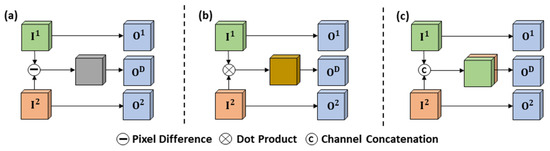
Figure 1.
The existing commonly used fusion methods of multi-task SCD. (a) Bi-temporal pixel difference. (b) Bi-temporal dot product. (c) Bi-temporal channel concatenation.
Furthermore, the imbalance of different class quantities in the SS branch exerts a direct effect on the bias of prediction, and it is even more pronounced in the SCD. The most common approach is to perform data augmentation and resampling for the training samples that belong to small quantities. For example, Tang et al. [41] achieved class quantity balance in the training dataset by employing semi-supervised learning to expand the small samples. Zhu et al. [42] designed a global hierarchical sampling mechanism to alleviate the negative effects of class imbalance. Although the processing of data levels is an effective way, it can also cause the network’s overfitting to specific samples from minority classes [43]. In contrast, improving the loss calculation with penalty weights to optimize training serves as a superior approach for SCD in class rebalancing. Xiang et al. [44] and Niu et al. [45] obtained promising results in multi-task SCD by assigning specific weights in the joint loss function. Nevertheless, the above-mentioned specific weights are primarily assigned manually rather than adaptively, and numerous approaches have overlooked the distribution correlation between multiple and few samples, resulting in excessive skewness in the training process of small samples.
For the SCD method’s application, pixel-level SCD datasets based on HR images are very scarce due to constraints in standardization and the difficulty of production. Moreover, only a few researchers have explored the applicability of multi-task SCD methods in the field of a specific object’s SCD (the transition from a single class to multiple classes) [46]. Especially in recent years, cropland’s non-agriculturalization is one of the significant concerns in the management and protection of food security, and it has become a focal point for accurate detection of cropland change using HR images in the agricultural remote sensing field [47,48,49]. Liu et al. [50] detected the changes in cropland by using the method of BCD and proposed the first dataset of cropland change detection based on HR images, but their work was only limited to detecting change regions and lacked the ability to identify non-agricultural types. Thus, it is worthwhile to delve further into the application of multi-task SCD methods in cropland’s non-agricultural detection in HR images.
In this study, we propose a multi-task consistency enhancement network (MCENet) for SCD in bi-temporal HR images. The main contributions are as follows:
- (1)
- We propose a novel network for SCD, and the network is developed using the architecture of encoder-fusion-decoder based on multi-task learning. In the encoder, we design a stacked Siamese backbone that combines CNN and Transformer, which reduces the probability of miss detection while ensuring precise segmentation in the information detail;
- (2)
- To mitigate false detection arising in non-changing regions and enhance the results’ integrity representation of change features, we introduce a multi-task consistency enhancement module (MCEM) and adopt a method of cross-task mapping connection. Moreover, we design a novel joint loss to better alleviate the negative impact of class imbalance;
- (3)
- We propose a novel pixel-level SCD dataset about cropland’s non-agricultural detection, the non-agriculturalization of Fuzhou (NAFZ) dataset, which is constructed based on historical images from three distinct areas in Fuzhou. For the NAFZ dataset, we explore the suitability and performance of the proposed network for identifying non-agricultural types in HR images.
The rest of this study is organized as follows: Section 2 describes the details of the proposed method in this study. Section 3 introduces the experimental datasets, evaluation metrics, and details. Section 4 expresses the experiment results of each dataset and the analysis of comparative networks. Section 5 further delves into the method and discusses the results, and Section 6 provides the conclusions of this work.
2. Methodology
2.1. Overall Architecture of Network
The overall architecture of MCENet is shown in Figure 2. Our network is an encoder-fusion-decoder architecture based on multi-task learning. The details of the network are as follows: In the encoder part, we adopt a Siamese backbone with weight sharing to extract multi-level dimension features from bi-temporal HR images, respectively. In the fusion part, we introduce a multi-task consistency enhancement module (MCEM) to achieve bi-temporal feature fusion. In the decoder part, the multi-branch decoder structure is used for feature information interpretation and output of predicted results, which are divided into single branches of BCD and dual branches of SS.
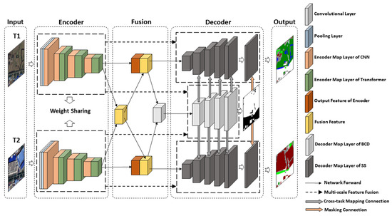
Figure 2.
The overall architecture of MCENet.
2.2. Encoder of MECNet
Transformer is capable of facilitating the capture of global context information from the specific deep feature sequence, which can compensate for the limitations of the convolutional kernel receptive field. Accordingly, we propose a network construct strategy, i.e., the backbone is partitioned into multiple map layers, and the number of feature sequences is insufficient in the channel of the initial map layers. Thus, in the first map layer, we employ a traditional CNN block to acquire channel features with a certain depth. In subsequent map layers, CNN blocks and Transformers are stacked orderly, which ensures that each map layer can model local and global features synchronously and reduce information loss. On that basis, we construct a stack Siamese backbone that combines CNN and Transformer as encoders for feature extraction. Figure 3 illustrates the encoder’s architecture.
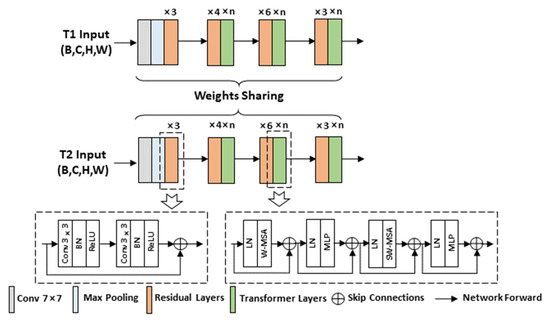
Figure 3.
The encoder’s architecture of MCENet.
Specifically, a single backbone comprises four composite blocks as feature map layers. ResNet34 [51] serves as the standard backbone, and the first block is comprised of a convolution layer with a kernel size of 7 × 7 and a maximum pooling layer with a kernel size of 3 × 3. Next, we use two convolution layers with a 3 × 3 kernel size to form the residual connection, and the number of residual layers is set to 3. In the subsequent three blocks, we stack the Transformer layer alongside the residual layer for each map dimension. In this process, to reduce parameter computation while ensuring performance, we adopt Swin-Transformer [52] as the Transformer layer, where the window size of multi-head self-attention is set to 8 × 8.
2.3. Multi-Task Consistency Enhancement Module
For the current issues and inspired by common fusion methods in BCD, we adopt a reasonable and effective strategy: We obtain the bi-temporal synthesis feature through fusion, and the deep fusion feature not only emphasizes the prior change location information between bi-temporal images but also encompasses the identical semantic representation of corresponding surfaces in non-changing regions. We incorporate the fusion feature into SS branches to improve SS branches’ learning of non-changing mapping features, then further enhance the pixel-level semantic consistency at the corresponding location in non-changing by employing an interactive attention module. During the training process, SS branches can more effectively learn the pixel value in non-changing between bi-temporal images by combining the fusion feature, thereby promoting SS branches to reduce non-changing’s false detection and improve spatial integrity segmentation of change. Compared with only performing opposite interactions between SS branches, this strategy considers the integrated relationship among multiple branches instead of isolating the fusion branch. This approach further facilitates the network’s learning of the similarity of identical surfaces and the distinctiveness of features among different surfaces between bi-temporal images.
On that basis, the multi-task consistency enhancement module (MCEM) is introduced, and the architecture is presented in Figure 4. Specifically, given input features , where denotes the number of channels of a single input feature, and W express the height and width of single input feature. First, we obtain the deep fusion feature through bi-temporal pixel difference:
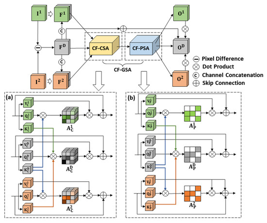
Figure 4.
The architecture of MCEM. (a) the architecture of CF-CSA. (b) The architecture of CF-PSA.
We take as channel feature to incorporate into respectively, to obtain :
To further enhance the ability to focus on change foreground information and identify the commons of semantic feature among the objects in corresponding spatial positions in non-changing regions, we exploit channel and spatial self-attention [53] and propose a new attention module, cross-feature global self-attention (CF-GSA). CF-GSA consists of two parts: cross-feature channel self-attention (CF-CSA) and cross-feature position self-attention (CF-PSA). At the step of CF-CSA, we create six independent feature vectors from and three independent feature vectors from . The above-described feature vectors are obtained by introducing several trainable parameter matrices to and and transforming through linear projection, and each vector represents different spatial map results for the corresponding feature in the same dimension:
where denote the trainable parameter matrices of and denote the trainable parameter matrices of .
For SS branches, the similarity attention matrix is obtained by the dot product and the operation of softmax between and , respectively. Compared with only interaction between SS branches, utilizing a feature vector from the BCD branch for conducting cross-attention matrix can ensure semantic consistency in non-changing regions while reducing the burden introduced by semantic features in change regions from the opposite branch. Furthermore, this operation utilizes synchronously the prominent pixel values in the change regions from the fusion feature, prompting SS branches to identify change regions. For BCD branches, we generate the similarity parameter matrix belonging to in the same manner by adopting and . enables a more refined adjustment of similarity between bi-temporal images by cascading the attention matrix generated from the feature vector of SS branches, which can enhance the ability to identify changing regions of the BCD branch.
In the first step of CF-CSA, the similarity parameter matrix at the channel level is computed, and channel feature vectors satisfy and :
In the next step of CF-PSA, the similarity parameter matrix is computed, and position feature vectors are expressed as and :
Finally, we employ skip connection to generate the dual map outputs for SS branches and utilize dot product to generate the fusion output for the BCD branch:
2.4. Decoder of MCENet
Figure 5 depicts the multi-task decoder structure of MCENet. From the overall design, we conform to the multi-task integrated strategy [22] to preserve the integrity of information in the feature interpretation process.
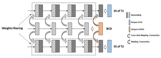
Figure 5.
The multi-task decoder architecture of MCENet.
Specifically, an equal number of feature map layers in the decoder is constructed as an encoder to achieve multi-scale skip connections. Moreover, in the design of the decoder’s branches, the dual subtask branches with weight sharing for SS are set to increase the robustness of the network and reduce the calculation of parameters. With the aim of further increasing the final accuracy and fitting performance of SS branches, we adopt cross-task mapping connections that take each decoder map layer of the BCD branch and incorporate it into the corresponding map layers of SS branches, which drives SS branches to learn more abundant multi-level semantic consistency features of non-changing surfaces. Lastly, the predicted result of the BCD branch is masking connected with the final map layer of the SS branches through vector multiplication. In this study, the traditional design is followed, each decoder layer selects upsampling with bilinear interpolation, and the size of the convolution kernel is set to 1 × 1.
2.5. Loss Function
The traditional multi-task SCD network calculates the loss of SS branches () and BCD branch (), respectively, then adds them together as the final multi-task joint loss function. For real datasets, however, the imbalance of classes in bi-temporal images can affect the optimization of each branch’s loss, which affects the overall performance of the network. To address the above-mentioned problem, we assign specific adaptive weight to SS branches () and BCD branches (), respectively, and add an auxiliary loss () to develop a novel multi-task joint loss function ( for the network’s backpropagation:
where denotes the loss function with adaptive weights of the SS branches of T1 and T2, respectively, denotes the loss function with adaptive weight of the BCD branch; and denotes the auxiliary loss function.
To be more specific, in the training samples, we set the changing regions as positive pixels and the non-changing regions as negative pixels. For , we set the total number of segmentation classes in positive pixels as , and in the single batch of training, we count the number of total pixels , positive pixels number and each segmentation type in positive pixels , respectively. First, the proportion of and is computed to enhance the overall skewness towards the classes with fewer classes; when is small, the proportion will increase, and higher values are assigned to the fewer classes. Subsequently, the inverse distribution proportion of and is obtained to further increase the accuracy of the fewer classes in positive class; when is small, the inverse distribution proportion will increase, and higher values are assigned to the fewer segmentation types in positive class. Lastly, the final trade-off weight of a single SS branch is determined by summing up:
where denotes the attribute number for the corresponding class. And the loss function formula for single SS branches is as follows:
where denotes the number of samples in the single batch of training, denotes the distribution of ground truth for -th class in -th SS branch, and denotes the probability distribution of predicted results for -th class in -th SS branch.
For , non-uniformity of the positive and negative pixel proportions is the direct cause of the detection of the network’s instability between changing and non-changing. Thus, in the single batch of training, the positive pixels proportion and the negative pixels proportion in total pixels are obtained, and they are selected as trade-off weights and , respectively.
The final loss function formula of BCD branch is as follows:
where and denote the distribution of ground truth of positive and negative samples, respectively, and denote denotes the probability distribution of predicted results of positive and negative samples, respectively.
To further strengthen the conformity of non-changing between the predicted results of SS branches, we introduce the contrastive loss [54] based on Euclidean distance as the auxiliary loss to minimize the distance metric in the non-changing pixels between bi-temporal images and alleviate the false detection of non-changing caused by pseudo-change:
where and denote pixel feature vectors of the predicted results from SS branches, respectively; denotes the pixel value of the corresponding position of the predicted results from the BCD branch; and denotes the threshold parameter.
3. Experiment Datasets and Evaluation Metric
3.1. Experiment Datasets
In this study, we conducted experiments using three pixel-level SCD datasets created by HR remote sensing images, including the SCEOND dataset [55], the HRSCD dataset [26], and the NAFZ dataset. The images in these datasets are derived from diverse platforms or sensors, and all of them have corresponding pixel-level labels of ground truth. The SECOND and HRSCD datasets are two open-source datasets that serve as crucial references for the current method research on SCD. And the NAFZ is a manual, self-created dataset primarily used to evaluate the applicability of SCD methods across cropland’s non-agricultural detection. The relevant brief information about the datasets is presented in Table 1.

Table 1.
The relevant brief information about the SECOND, HRSCD, and NAFZ datasets.
3.1.1. The SECOND Dataset
SECOND is a SCD dataset dedicated to refined pixel-level SCD research in LULC for multi-source HR images, covering areas including Hangzhou, Chengdu, Shanghai, and Nanjing, China. The dataset comprises 2968 pairs of tile image samples with a spatial resolution of 0.5 m to 3 m and a size of 512 × 512 pixels. There are seven basic LULC surface categories that involve both common natural and man-made in the labeled sample, including non-changing, non-vegetated surfaces (primarily referred to as bare land and impervious surfaces), low vegetation, trees, buildings, water, and playgrounds. As a benchmark dataset with excellent quality, the results of the SECOND dataset could have great significance in validating the feasibility of SCD methods. In this experiment, we preprocessed the SECOND dataset by performing regular cropping of bi-temporal images to the size of 256 × 256 pixels, and the processed dataset comprises 11,872 pairs of bi-temporal images for use in the experiment. We further adopted the random split ratio of 8:1:1 to divide the dataset into a training set, a validation set, and a test set, with 9490 pairs for training, 1192 pairs for validating, and 1190 pairs for testing. Figure 6 presents the partial visualization of images and ground-truth labels in the SECOND dataset.
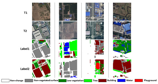
Figure 6.
The partial visualization of images and ground truth labels of the SECOND dataset.
3.1.2. The HRSCD Dataset
HRSCD is a SCD dataset based on HR images from the BD ORTHO database, which covers areas covered by images in several regions of France. The original dataset covers land cover semantic segmentation labels and binary change labels for bi-temporal images, which comprise 291 pairs of complete images with a spatial resolution of 0.5 m and a size of 10,000 × 10,000 pixels. HRSCD’s satellite image source is completely different from SECOND, so it can validate the applicability of SCD methods on different source HR images. In the experiment, the origin segmentation label and the binary change label were merged through a spatial overlay and filter, and then the semantic change labels were obtained. The classes of land cover include artificial surfaces, agricultural areas, trees, and water. On that basis, we preprocessed the HRSCD dataset by performing regular cropping of bi-temporal images to the size of 256 × 256 pixels, and the processed dataset comprises 6830 pairs of bi-temporal images for use in this study’s experiment. Furthermore, the random split ratio of 8:1:1 was adopted to divide the dataset into the training set, the validation set, and the test set, including 5470 pairs for training, 680 pairs for validating, and 680 pairs for testing. Figure 7 presents the partial visualization of images and ground-truth labels in the HRSCD dataset.
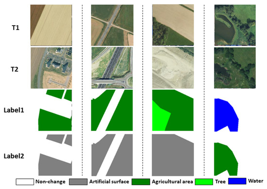
Figure 7.
The partial visualization of images and ground truth labels of the HRSCD dataset.
3.1.3. The NAFZ Dataset
Fuzhou is one of China’s coastally developed cities, with the most prominent feature being the scarcity of plains, which consequently results in a particularly limited availability of cropland resources. In recent years, the development of urbanization and industrial transformation has led to the phenomenon of non-agricultural cropland in plain areas. Accordingly, this study only examines the applicability of SCD methods for non-agriculturalization of cropland in HR images, and we created the non-agriculturalization of Fuzhou (NAFZ) dataset using images covering Fuzhou’s typical areas.
The NAFZ dataset was derived from Google Earth HR images. Noteworthy, the images we obtained through screening were slightly affected by external factors (e.g., cloud cover and shooting angles), and we strictly followed the general guidelines of Google Earth (https://www.google.com/permissions/geoguidelines/) (accessed on 17 November 2022). The images in the dataset cover three different areas in Fuzhou, with two located in Changle and one in Minhou. Over the past few years, due to the construction of Binhai New Area and State-Level Development New Area, the non-agricultural phenomenon of cropland in these areas has also been the most typical. The spatial resolution of each image we selected is 0.6 m, and we made semantic labels of cropland change and non-agricultural types by manual labeling. In the above-described dataset, we design seven classes of non-agricultural types (i.e., non-changing, cropland, tree, water, building, road, and bare land). In practical situations, the non-agricultural types are mostly associated with construction purposes, whereas other types are relatively less common, which also makes the dataset subjected to the obvious challenge of the class imbalance problem. In this experiment, bi-temporal images in the NAFZ dataset were preprocessed by performing slip windows cropping to the size of 256 × 256 pixels, and we expanded the number of positive samples (the samples containing cropland changes) through the random rotation operation (including 90°, 180°, and 270° rotation and mirror inversion). The final experiment dataset includes 21,585 pairs of bi-temporal images, and the number of positive samples includes 15,973 pairs. We further adopted the random split ratio of 7:2:1 to divide the dataset into the training set, validation set, and test set, with 15,110 pairs for training, 4315 pairs for validating, and 2160 pairs for testing. The visualization of origin images, labels, and specific information of the NAFZ dataset is presented in Figure 8 and Table 2.
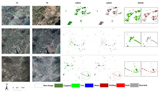
Figure 8.
The visualization of images and ground truth labels of the NAFZ dataset.
Table 2.
The specific information of the NAFZ dataset’s images.
3.2. Evaluation Metric
In this study, we adopted eight objective metrics to evaluate the performance of the network in SCD, including overall accuracy (OA), Intersection over the Union of Change (IoUc), mean Intersection over the Union (mIoU), F1 score of overall results (F1), F1 score of SS in change regions (FSCD), Kappa of SS in change regions (Kappa), separated Kappa coefficient (Sek), and overall score (Score).
We set denotes the value of the predicted class, denotes the value of the real class (while non-changing is represented as 0), denotes the total count of all pixels, and denotes the count of pixels that are predicted correctly. OA is used to assess the overall performance of the network:
mIoU is computed by the mean value of Intersection over the Union between non-changing (IoUnc) and change (IoUc):
F1 is used to evaluate the accuracy of all class in semantic segmentation, and it is calculated by the overall precision (P) and recall (R):
FSCD is used to evaluate the accuracy of multi-class semantic segmentation in change regions, and it is calculated by the positive samples’ precision (PSCD) and recall (RSCD):
To comprehensively evaluate the performance in positive samples while preventing significant overly dominant effects caused by negative samples on the traditional metric, we adopted the metric of and :
3.3. Implementation Details
The experiments were all implemented by employing PyTorch on Windows 11, and we accelerated the training of network by using the NVIDIA GeForce RTX 3070 GPU. Moreover, stochastic gradient descent with momentum (SGDM) was selected as a network optimizer with a weight decay of 0.005 and a momentum of 0.9 for setting the training parameters. The initial learning rate for network training and the learning rate decay were set to 0.001 and 0.9, respectively.
4. Experiment Results and Analysis
4.1. Comparative Networks Introduce
We adopted several typical CD networks possessing excellent characteristics for performance comparison. The selected comparative networks are described as follows:
- The benchmark architectures of CD networks are: (1) The series of Siamese FCN [23]: The Siamese FCN serves as the baseline network for BCD. In this study, the applicability of Siamese FCN in SCD was investigated by only modifying its architecture at the output layers. Specifically, we adopted the fully convolutional Siamese concatenation network (FC-Siam-Conc) and the fully convolutional Siamese difference network (FC-Siam-Diff) that have been extensively employed in existing research. (2) The series of HRSCD networks [22]: baseline networks and different architectural design strategies for SCD were proposed by Daudt et al. It provides a basic reference for evaluating the proposed network. In this study, we selected three networks designed according to multi-task strategies, including the multi-task direct comparison strategy (HRSCD-str.1), the multi-task separate strategy (HRSCD-str.3), and the multi-task integrate strategy (HRSCD-str.4);
- FCCDN [26]: A multi-task learning-based feature constraint network. The nonlocal feature pyramid and a strategy of self-supervised learning are adopted in this network to achieve SS for bi-temporal images. It is characterized by SS-guided dual branches and restricts the decoder from generating CD results;
- BIT [34]: A network that takes the first attempt to apply CNN and Transformer as the backbone for CD. In this network, CNN is independently adopted to capture bi-temporal shallow features and corresponding fusion features, while a single Transformer backbone is leveraged to extract high-level fusion features;
- PCFN [28]: A Siamese post-classification design-based multi-task network. It guides dual branches of SS by incorporating the encoder’s multi-scale fusion features, and it generates the results of change types by only merging the output layer of the SS branch in the decoder;
- SCDNet [27]: A multi-task network based on Siamese U-Net. Compared with PCFN, it also exploits the multi-scale fusion features of the encoder to guide SS branches. In the decoder, however, the network does not employ an independent branch for BCD and optimizes it through the corresponding loss function;
- BiSRNet [40]: A novel SSCD-l architecture proposed by Ding et al. based on the late fusion and subtask separation strategy. This novel benchmark architecture of multi-task SCD employs Siamese FCN as the backbone. Moreover, the method introduces a cross-temporal semantic reasoning (Cot-SR) module to develop information correlations between bi-temporal features;
- MTSCDNet [56]: A multi-task network based on Siamese architecture and Swin-Transformer. Similar to the strategy adopted in this study, this network gains the attention map of the deep change feature by adopting the spatial attention module (SAM) and then cascades into subtasks in the channel dimension, such that the network is endowed with a better ability to recognize change regions while maintaining consistency in non-changing regions.
4.2. Results on the SECOND Dataset
In the quantitative results of the SECOND dataset in Table 3, FC-Siam-Concat, FC-Siam-Diff, and HRSCD-str.4 outperformed other benchmark networks, which is partially attributed to the implementation of a multi-scale fusion strategy between the encoder and the decoder in the BCD branch. FCCDN exploited the correlation among branches, which led to a certain improvement of at least 2.67% Sek and 2.23% Score compared with the benchmark networks. BIT, PCFN, and SCDNet achieved significant strides in a wide variety of metrics, especially in Sek, where BIT improved by 2.47% over FCCDN, which can demonstrate the critical role of Transformer in the global feature extraction process. The Sek of PCFN and SCDNet was improved by 2.97% and 1.69%, respectively, compared with that of FCCDN, which can demonstrate the effectiveness of utilizing the multi-level map features of the BCD branch to guide SS branches. Notably, the three above-mentioned networks pursue distinct approaches, either focusing on enhancing feature extraction or performing branch task corrections, whereas these auxiliary methods are not properly integrated, such that none of them achieve superior results. BiSRNet and MTSCDNet considered temporal and spatial relationships to enhance classification performance and address the issue of false detection in non-changing regions, thus achieving significant results. MTSCDNet outperformed BiSRNet by 3.89%, 1.84%, and 0.68%, respectively, in the metrics of IoUC, FSCD, and Sek. The above result can indirectly support the idea that designing multi-branch interactivity based on Transformer is more effective than relying solely on CNN and dual branches for reverse interaction. In contrast, MCENet achieved optimal quantitative results on the SECOND dataset, with the overall performance evaluation reaching 88.42% OA, 52.21% F1, 22.06% Sek, and 37.41% Score.
Table 3.
Quantitative results of different networks on the SECOND dataset.
In the partial visualization results of Figure 9, all the benchmark networks exhibit incompleteness and fragmentation issues in change region detection, and they also have confusion in identifying low vegetation and trees (e.g., (1) in Figure 9). FCCDN, PCFN, and SCDNet encounter segmentation ambiguity when detecting high-density and non-obvious buildings, and the ability to detect partial classes is unsatisfactory, especially playgrounds (e.g., (2) and (4) in Figure 9). It also illustrates the shortcomings of CNN to some extent. While BIT overcomes the shortcoming in feature extraction, the lack of connection among branches leads to semantic false classification and miss detection in complex regions (e.g., (2) and (3) in Figure 9). The results of BiSRNet reveal that its ability to differentiate between different surfaces with similar spectral features is not highly satisfactory, including semantic confusion between non-vegetated surfaces and buildings (e.g., (1) in Figure 9). Furthermore, BiSRNet has also exhibited similar issues of target omission as the baseline network (e.g., (2) and (3) in Figure 9). MTSCDNet has improved in these issues, but there are also cases of water being missed (e.g., (3) in Figure 9). Through the corresponding visualization results of MCENet, it can be observed that the issues encountered by other networks are effectively eliminated or alleviated by MCENet. Most importantly, MCENet demonstrates superior performance in integrity segmenting of change regions and significantly alleviating the pseudo-change phenomena in the surface with intraclass differences (e.g., (1) in Figure 9). Notably, MCENet demonstrates a remarkable ability to completely identify and segment targets, such as water, which other networks failed to achieve accurately.
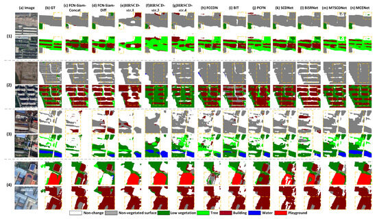
Figure 9.
Partial visualization results of different networks on the SECOND dataset. (a) images. (b) ground truth. (c) FCN-Siam-Concat. (d) FCN-Siam-Diff. (e) HRSCD-str.1. (f) HRSCD-str.3. (g) HRSCD-str.4. (h) FCCDN. (i) BIT. (j) PCFN. (k) SCDNet. (l) BiSRNet. (m) MTSCDNet. (n) MCENet.
4.3. Results on the HRSCD Dataset
Table 4 lists the quantitative results on the HRSCD dataset. The detection results of different networks could not reach a high level due to the presence of certain noise and erroneous annotations in the ground-truth labels of HRSCD. The experiments with the benchmark network indicated that using traditional methods of CD yielded suboptimal results, which suggested that more meticulous and reasonable network design is required. Moreover, FCCDN and SCDNet failed to achieve favorable results, and they were even worse than parts of the benchmark networks (only achieving 2.88% and 5.09%). Noteworthy, PCFN, BiSRNet, and MTSCDNet gained significantly better metric results; the commonality among the three networks was dependent on their focus on semantic correlations between multiple branches, and the value of this idea can be readily discerned from the quantitative results. For the results of mIoU and F1, MTSCDNet was 0.7% and 3.1% higher than BiSRNet, respectively, which suggested that the parallel combination of guiding SS branches through the deep fusion feature for simultaneous optimization can possess high effectiveness in the HRSCD dataset. In contrast, MCENet obtained the optimal results, with 61.73%, 14.87%, and 30.61% in FSCD, Sek, and Score, respectively. Furthermore, the results of other metrics were significantly better than those of other networks.
Table 4.
Quantitative results of different networks on the HRSCD dataset.
The partial visualization results of the HRSCD dataset, as presented in Figure 10, indicated that parts of the benchmark networks, including FCCDN and SCDNet, were subjected to severe false detection (e.g., (1) in Figure 10). These methods cannot overcome the issue of pseudo-changes arising from seasonal transitions in cropland. Furthermore, PCFN, BiSRNet, and MTSCDNet are relatively poor in suitability between change regions and semantic classes. Furthermore, MCENet can show its superiority by effectively alleviating the issue of pseudo-changes and well-identifying genuine change regions. It also possesses the remarkable ability to reduce semantic false detection and prevent adhesive effects in dense regions. For instance, it obtained the identity of trees’ cover areas and distinguishing roads that remained unchanged (e.g., (2) and (4) in Figure 10). Compared with other networks, MCENet can ensure better semantic consistency recognition while enhancing fine-grained spatial differentiation of targets, thus reducing the situation of fragmented and blurred detection patches.
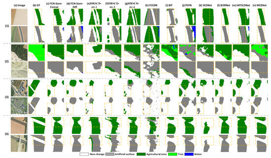
Figure 10.
Partial visualization results of different networks on the HRSCD dataset. (a) images. (b) ground truth. (c) FCN-Siam-Concat. (d) FCN-Siam-Diff. (e) HRSCD-str.1. (f) HRSCD-str.3. (g) HRSCD-str.4. (h) FCCDN. (i) BIT. (j) PCFN. (k) SCDNet. (l) BiSRNet. (m) MTSCDNet. (n) MCENet.
4.4. Results on the NAFZ Dataset
NAFZ is a SCD dataset that transforms from a single element to multiple elements, which is different from the other two datasets. Thus, the approach of using overall metrics is somewhat one-sided, and it requires more specific metrics to evaluate the network performance. The quantitative results of Table 5 indicated that HRSCD-str.1 consistently performed lower than other networks across a wide variety of metrics. This result suggested that the approach of detecting changes after comparing classification maps may exhibit poor feasibility in cropland change detection, leading to a higher likelihood of false detections (with a Sek and Score of only 4.18% and 21.19%, respectively). In the above-mentioned networks, PCFN and BiSRNet yielded relatively superior outcomes, achieving Seks of 20.10% and 20.92%, respectively. In contrast, MCENet was most consistent with actual occurrences of cropland changes and identified the non-agricultural types (with FSCD, Sek, and Score of 68.31%, 21.67%, and 37.28%, respectively), thus demonstrating better transferability and applicability of our network in the work of cropland’s non-agricultural detection based on HR images. Nevertheless, in the details, MCENet did not achieve optimal quantitative results on OA, which suggested that MCENet can also have slight limitations in comprehensive analysis. Furthermore, the above-described situation largely arises from the negligence of these metrics in emphasizing the distribution accuracy of positive samples for the NAFZ dataset. While FCCDN achieves better results in OA, it can perform relatively poorly when considering detailed indicators. Specifically, it achieved only 23.00% and 38.75% on IoUC and Kappa, respectively, a situation that reaffirms the above reasons. In general, the proposed network possesses superior suitability for the task of non-agriculturalization.
Table 5.
Quantitative results of different networks on the NAFZ dataset.
The visualization results of Figure 11 and the quantitative results suggested that PCFN can perform exceptionally well in recognizing non-agricultural types, whereas it also faces a significant problem of over-detection (e.g., (2) and (4) in Figure 11), which can arise from the lack of capture of global information. The results of BiSRNet are easily discernible, which can reveal its excellent spatial fine-grained aggregation ability, whereas it is subjected to significant difficulty in identifying minority classes, for example, the surfaces of water and roads (e.g., (3) and (4) in Figure 11). Moreover, MCENet has the advantage of having a fine segment of cropland change regions (e.g., (2) and (3) in Figure 11). MCENet has a strong discriminatory ability in cases of homogenous spectral characteristics of cropland and bare land. In contrast, MCENet can also better detect the surfaces of roads and water with relatively lower quantities in the dataset (e.g., (3) and (4) in Figure 11).
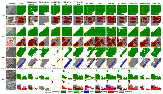
Figure 11.
Partial visualization results of different networks on the NAFZ dataset. (a) images. (b) ground truth. (c) FCN-Siam-Concat. (d) FCN-Siam-Diff. (e) HRSCD-str.1. (f) HRSCD-str.3. (g) HRSCD-str.4. (h) FCCDN. (i) BIT. (j) PCFN. (k) SCDNet. (l) BiSRNet. (m) MTSCDNet. (n) MCENet.
5. Discussion
5.1. Evaluation of MCEM
We maintained the same design structure as other parts within the network and equally compared MCEM with five fusion methods that have been employed in existing SCD research to evaluate the performance of MCEM in enhancing semantic consistency in non-changing regions. The compare methods fall into two major categories: one comprises traditional fusion methods that are derived from BCD, which cover bi-temporal pixel difference, bi-temporal dot product, and bi-temporal channel concatenation (we set bi-temporal features as and , and the above methods can be briefly expressed as , and , respectively). The other category involves fusion methods of two optimized designs, including fusion feature guide (FFG) module and the Cot-SR module. Furthermore, the specific structures are depicted in Figure 12.
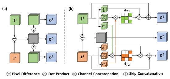
Figure 12.
The fusion methods of two optimized designs. (a) FFG module. (b) Cot-SR module.
The experimental results of Table 6 indicated certain differences in the quantitative values of , and , respectively. Although all three methods originated from the basic design of BCD, their application in SCD has not achieved our expected outcomes. The reason for this result is that no further attention is paid to the semantic correction relationship between bi-temporal images, which prevents the network from fully grasping and incorporating semantically consistent features of the non-changing regions. The visualization results indicated that none of the above three methods effectively dealt with the semantic alignment of non-changing’s features between bi-temporal images, thus preventing SS branches of the network from connecting to the commonalities shared by these features, e.g., there were semantic false detections of non-vegetated surface, agricultural area, and bare land in (1), (4), and (5) of Figure 13 due to spectral intraclass differences. Furthermore, in these three methods, demonstrated relatively favorable results for change regions detection, with minimal quantification result fluctuations and fewer issues of both misses of false detection, which can also help us use as a baseline reference for innovative design.
Table 6.
Quantitative results of different fusion methods on the SECOND, HRSCD, and NAFZ datasets.
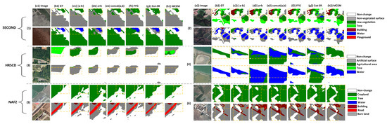
Figure 13.
Partial visualization results of different fusion methods on the SECOND, HRSCD, and NAFZ datasets. (a1,a2) images. (b1,b2) ground truth. (c1,c2) . (d1,d2) . (e1,e2) . (f1,f2) FFG. (g1,g2) Cot-SR. (h1,h2) MCEM.
FFG and Cot-SR pertain to two different improvement designs. The FFG module directly incorporates fusion features into dual branches, whereas the Cot-SR module interacts attention feature vectors from different spatial domains between dual branches. The results indicated that FFG outperformed Cot-SR on the whole. Compared with SS branch interactive mapping in Cot-SR, fusion branch mapping in FFG can enhance the semantic pixel information of change regions, which can lead to better results in change extraction. Also, SS branches can increase the semantic consistency of non-changing objects by incorporating untransformed pixel information from fusion features. And this has been corroborated in existing research [44,56]. But there has also been a certain semantic confusion in identifying surface types; the situation with Cot-SR is more severe (e.g., (2), (3), and (4) in Figure 13) and even falls below traditional methods in some metrics. This exposes that while Cot-SR can enhance the common features in SS branches in non-changing regions, the risk of redundant semantic features in change regions in the opposite branch is still surviving due to only processing between SS branches.
On that basis, our MCEM introduces CF-GSA. Like Cot-SR, we use independent feature vectors as the fundamental units. But the distinction in our approach is that we opt to employ vectors belonging to the BCD branch for synchronous interaction mapping with SS branches instead of reverse processing between SS branches. This design effectively addresses the issue of semantic feature redundancy present in Cot-SR. Furthermore, the design of CF-GSA enhances the module’s attention in both channel-level and spatial-level dimensions, which is a unique advantage not found in other fusion methods. Compared with the commonly used methods, the network with MCEM improves 1.73%, 0.73%, and 0.42% at least in Sek and 1.45%, 0.53%, and 0.54% at least in Score on the three datasets, respectively. Compared with two improved methods, the network with MCEM improved 0.72%, 0.67%, and 0.30% at least in Sek and 0.59%, 0.56%, and 0.36% at least in Score on the three datasets, respectively. The quantitative results demonstrate that the overall network performance’s improvement benefits from MCEM. And the visualization results show that MCEM enhances the network’s ability to capture the integrity change features effectively and further enhance the semantic consistency in non-changing regions (e.g., (1), (4), and (5) in Figure 13), especially the judgement of semantic information between the class of cropland and bare land in (5) of Figure 13. Even more surprising is that in terms of multi-class segmentation performance, the minimum improvement was 1.68%, 0.56%, 0.55%, 0.54%, and 1.61% in FSCD, respectively, after using MCEM. In contrast, it can be observed that the network with MCEM achieves superior segmentation of buildings with varying degrees of illumination interference and demonstrates excellent discrimination between non-vegetated surfaces and low vegetation (e.g., (1) and (5) in Figure 13).
From a methodological perspective, MCEM only belongs to an effective and versatile SCD network’s internal design. However, for specific requirements such as non-agricultural detection, additional auxiliary conditions can be incorporated to enhance prediction accuracy further, such as integrating parcel information, phenological knowledge, or change information transfer to construct innovative end-to-end approaches [57,58,59].
5.2. Evaluation of Proposed Loss Function
To evaluate the performance of the proposed joint loss function in this study, we quantitatively compare it with joint loss functions that have already been applied to SCD. The comparative loss functions include:
- Loss-a: The joint loss function without adaptive weights ();
- Loss-b: The joint loss function with adaptive weights ();
- Semantic consistence loss (SCL) [44]: SCL is a similarity measurement loss function proposed by Ding et al., based on cosine similarity theory. It calculates the difference between semantic mapping results and change labels through the cosine loss function;
- Tversky loss (TL) [56]: TL is the loss function designed by Cui et al., based on the Tversky index theory, specifically aimed at mitigating class imbalance issues. It relies on increasing the weight of negative pixels to reduce the effect of non-changing samples.
The metric results of Score reveal that the overall performance of the network has significantly improved after using Joint loss-b (Table 7). Compared with Loss-a, the accuracy values of Score on three datasets increase by 1.23%, 0.80%, and 1.01%, respectively. For the visualization results, it is evident that the network with Loss-b can effectively overcome false detection issues caused by surfaces with semantic consistency but with spectral pseudo change, for example, the low vegetation of the SECOND dataset and the artificial surface of the HRSCD dataset (e.g., (1) and (4) in Figure 14). Furthermore, it successfully enhances the detectability of surface categories that are either low in quantity or difficult to detect; for example, the playground of the SECOND dataset and the water of the NAFZ dataset (e.g., (2), (5), and (6) in Figure 14). The prediction outcomes across the three datasets demonstrate the robust applicability of the design of adaptive weights.
Table 7.
Quantitative results of different joint loss functions on the SECOND, HRSCD, and NAFZ datasets.
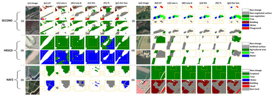
Figure 14.
Partial visualization results of different joint loss functions on the SECOND, HRSCD, and NAFZ datasets. (a1,a2) images. (b1,b2) ground truth. (c1,c2) Loss-a. (d1,d2) Loss-b. (e1,e2) SCL. (f1,f2) TL. (g1,g2) Our loss.
Comparing SCL and TL, it can be observed that the predicted results of SCL are superior to those of TL. Additionally, TL fails to achieve the results of Loss-a on the HRSCD and NAFZ datasets (only achieve 28.72% and 33.09% in Score, respectively). This situation can be attributed to differences in the measurement approach of the loss function, resulting in issues of applicability across different datasets. And the joint loss function we design in this study gains significant improvements across the metrics, which achieves optimal performance. In the visualization results of Figure 14, we can clearly see that the proposed loss can effectively handle the change surface that is difficult to identify, while also achieving a higher level of granularity in SS, especially in the detection of water. The proposed joint loss function demonstrates excellent recognition performance (e.g., (2), (3), and (5) in Figure 14). From the results of various loss functions, we can find that the intrinsic connection perspective of the joint loss function, SS and BCD, complements each other and optimizes together. As BCD undergoes optimization improvements, SS can concurrently gain enhancements [39,60].
5.3. Ablation Study
To evaluate the performance of the proposed auxiliary designs, respectively, in this study, we based them on MECM and conducted the ablation experiments in view of the network itself. The experiment designs for each group of ablation works are as follows:
- Model-a: We adopted the Siamese backbone of the standard Resnet34 encoder and the traditional multi-task joint loss function (Loss-a) as the baseline network in accordance with the architecture of the multi-task integrated strategy;
- Model-b: Based on Model-a, we adopted the proposed loss (our loss) in this study to analyze its effect on the overall network performance;
- Model-c: Based on Model-b, we adopted the proposed backbone that combines CNN and Transformer in this study to investigate its effect on the overall network performance;
- Model-d: Based on Model-c, we adopted the method of cross-task mapping connection and assembled the auxiliary designs involved in the above to explore its effect on the overall network performance.
Table 8 and Table 9 list the specific relevant settings and the quantitative results. First, we can observe that the proposed loss function has a positive effect on the performance of SCD from the quantitative results of MCENet-b on the three datasets. The most noticeable improvement is observed on the NAFZ dataset, with increases of 1.52%, 2.39%, and 1.93% on FSCD, Sek, and Score, respectively. In the corresponding visualization results of Figure 15, after employing the proposed joint loss function, the network can effectively detect playgrounds, trees, and water (e.g., (1), (4), and (6) in Figure 15), and all of these were classes with relatively fewer quantities in their respective datasets. It shows the benefits of the proposed loss function for the network’s training optimization. From (5) in Figure 15, Model-b exhibited better comprehensiveness in detecting change regions, which can further validate the beneficial effect of the proposed loss on the segmentation of positive samples.
Table 8.
Relevant settings of ablation experiments.
Table 9.
Comparison the results of ablation experiments on the SECOND, HRSCD and NAFZ datasets.
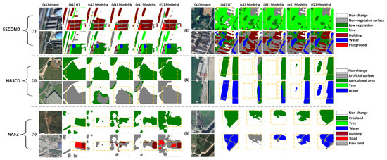
Figure 15.
Partial visualization results of ablation experiments on the SECOND, HRSCD, and NAFZ datasets. (a1,a2) images. (b1,b2) ground truth. (c1,c2) Model-a. (d1,d2) Model-b. (e1,e2) Model-c. (f1,f2) Model-d.
After using the proposed stacked backbone, the network’s overall performance for segmentation classes has significantly improved. Compared with Model-b, Model-c has increased by 1.50%, 2.25%, and 2.38% on Sek and by 1.05%, 2.27%, and 2.23% on Score on three datasets, respectively. For the ambiguous areas that difficult to judge and complex surfaces segmentation, Model-c presents superior performance, particularly dealing intricate features like narrow green belts and inundated water (e.g., (1), (2) and (4) in Figure 15). This is largely attributed to Transformer’s ability to capture global context information during the high-level feature extraction process.
Lastly, we adopted a cross-task mapping connection and assembled all the auxiliary designs. The design of the cross-task mapping connection promoted the SECOND and NAFZ datasets with slight accuracy gains. Moreover, on the HRSCD dataset, the improvements were most pronounced (improve by 6.89% FSCD, 3.99% Sek, and 3.35% Score). In the visualization, Model-d exhibits excellent consistency in preserving the entire range of change regions and achieves fine-grained separation between different surfaces (e.g., (3), (4), and (6) in Figure 15). Combined, the conclusion of evaluating in Section 4 further substantiates the notion that establishing more map-level connections from the BCD branch for associating and guiding SS branches is a highly effective approach. Moreover, the results obtained from Model-d indicate that map connections from the decoder lead to relatively better outcomes. Furthermore, an important detail worth noting is that, as seen in (1) and (5) in Figure 15, both the SECOND and the NAFZ datasets contain slight annotation errors in ground-truth labels. However, Model-d can compensate for these discrepancies and successfully detect the correct semantic classes. For example, in the result of (1) in Figure 15, our network can accurately identify the trees in the greenbelt as the class of trees instead of low vegetation, and in the result of (6) in Figure 15, our network can identify the class of changed cropland and the non-agricultural types of roads and bare land that are incompletely labeled.
We further set different Transformer layer combinations in the Siamese backbone based on Model-d to conduct evaluation. The quantitative results are presented in Table 10. From the results on three datasets, as the quantity of blocks in each layer increases, the performance of the network increases first and then tends to decrease. For the SECOND and HRSCD datasets, when the combination of Transformer blocks was set to (2, 2, 2), the network obtained the optimal quantitative results. For the NAFZ dataset, when the combination of Transformer blocks was set to (3, 3, 3), the network obtained the optimal quantitative results. To a certain extent, the phenomenon can arise from various factors (e.g., differences in the volume of training data and redundancy in the network’s internal parameters).
Table 10.
Quantitative results of different Transformer layer combinations in the Siamese backbone on the SECOND, HRSCD, and NAFZ datasets.
6. Conclusions
In this study, we proposed a multi-task consistency enhancement network (MCENet) for SCD in HR remote sensing images. Based on multi-task learning, we adopted the stacked Siamese backbone that combines CNN and Transformer as encoders. We designed two auxiliary methods to integrate into a network, i.e., a novel fusion module termed the multi-task consistency enhancement module and the design of a cross-task mapping connection in the decoder. Moreover, we introduced a novel multi-task joint loss function to alleviate the effect of the network’s training on class imbalances in quantity. To evaluate the performance of our network, we compared methods comprehensively, evaluated auxiliary modules, and performed an ablation study on two publicly available SCD datasets and a cropland non-agriculturalization dataset that was self-created. Through experiments, we drew the conclusions as follows: (1) Compared with different networks, MCENet exhibits superior performance in both quantitative metrics and visualization results, and it shows excellent applicability in cropland’s non-agricultural detection in HR images. (2) Compared with the commonly employed fusion methods and optimized fusion methods of SCD, the network with MCEM achieves optimal accuracy in results, thus demonstrating the effectiveness of MECM in semantic consistency enhancement of non-changing regions and high coincidence for real-life situations in detecting semantic transition, and it also maximizes the preservation of the integrity of change features. (3) Compared with the performance of different joint loss functions, the proposed joint loss function can not only increase the overall quantitative accuracy but also show significant optimization benefits for identifying minority classes across three various datasets. (4) Through ablation experiments, we demonstrated that the assembly of all the auxiliary designs in feature extraction, branch correlation, and joint loss function that are proposed in this study is beneficial for the network to achieve superior SCD results.
The current research on HR image change detection suggests that BCD has a relatively rich pixel-level benchmark dataset and a mature methodology system. In contrast, for SCD, which is in the preliminary stage of research, it still has the following challenges to be explored in future work: (1) Limitation of SCD datasets: there are some publicly available SCD datasets covering different data sources and application objects, including medium resolution-based urban land use change (Taizhou and Nanjing datasets) [61,62], scene-level semantic change (Mts-WH dataset) [63], and hyperspectral semantic change (Yancheng dataset) [64], whereas benchmark SCD datasets for refined pixel-level and multi-source images continue to be highly scarce. Accordingly, expanding the types and volume of pixel-level SCD datasets is helpful for the feasibility verification and further exploration of SCD methods. (2) Breakthrough of SCD methods: in the present study, there is still insufficient exploration in SCD methods. This is mainly evident in two aspects: on the one hand, we have focused excessively on improving the accuracy of change regions while facing bottlenecks in modeling change types. Although the proposed MCENet enhances the class segmentation ability, there are still limitations in insufficient modeling, which is worth exploring by using methods that can better characterize change types. Furthermore, the difficulties encountered in the production of datasets and the improvement of existing methods facilitate the exploration of new mentalities, and the application of weakly supervised and multi-modal learning based on a few samples are valuable development directions for future research on SCD.
Author Contributions
Conceptualization, X.W. and M.L.; methodology, H.L.; validation, D.H., R.W. and H.L.; formal analysis, D.H. and R.W.; writing—original draft preparation, H.L.; writing—review and editing, X.W. and M.L; funding acquisition, X.W. All authors have read and agreed to the published version of the manuscript.
Funding
This research was funded by the Fujian Science and Technology Plan Project (Grant No. 2022C0024) and the Fujian Water Science and Technology Project (Grant No. MSK202214).
Data Availability Statement
The SECOND and HRSCD datasets are available online.
Conflicts of Interest
The authors declare no conflict of interest.
References
- Fatemi Nasrabadi, S.B. Questions of Concern in Drawing Up a Remote Sensing Change Detection Plan. J. Indian Soc. Remote Sens. 2019, 47, 1455–1469. [Google Scholar] [CrossRef]
- Khelifi, L.; Mignotte, M. Deep learning for change detection in remote sensing images: Comprehensive review and meta-analysis. IEEE Access 2020, 8, 126385–126400. [Google Scholar] [CrossRef]
- Bai, T.; Sun, K.; Li, W.; Li, D.; Chen, Y.; Sui, H. A novel class-specific object-based method for urban change detection using high-resolution remote sensing imagery. Photogramm. Eng. Remote Sens. 2021, 87, 249–262. [Google Scholar] [CrossRef]
- Fang, H.; Guo, S.; Wang, X.; Liu, S.; Lin, C.; Du, P. Automatic Urban Scene-Level Binary Change Detection Based on A Novel Sample Selection Approach and Advanced Triplet Neural Network. IEEE Trans. Geosci. Remote Sens. 2023, 61, 5601518. [Google Scholar] [CrossRef]
- Xia, L.; Chen, J.; Luo, J.; Zhang, J.; Yang, D.; Shen, Z. Building Change Detection Based on an Edge-Guided Convolutional Neural Network Combined with a Transformer. Remote Sens. 2022, 14, 4524. [Google Scholar] [CrossRef]
- Zheng, Z.; Zhong, Y.; Wang, J.; Ma, A.; Zhang, L. Building damage assessment for rapid disaster response with a deep object-based semantic change detection framework: From natural disasters to man-made disasters. Remote Sens. Environ. 2021, 265, 112636. [Google Scholar] [CrossRef]
- Rui, X.; Cao, Y.; Yuan, X.; Kang, Y.; Song, W. Disastergan: Generative adversarial networks for remote sensing disaster image generation. Remote Sens. 2021, 13, 4284. [Google Scholar] [CrossRef]
- Wu, C.; Zhang, F.; Xia, J.; Xu, Y.; Li, G.; Xie, J.; Du, Z.; Liu, R. Building damage detection using U-Net with attention mechanism from pre-and post-disaster remote sensing datasets. Remote Sens. 2021, 13, 905. [Google Scholar] [CrossRef]
- Zhu, L.; Xing, H.; Zhao, L.; Qu, H.; Sun, W. A change type determination method based on knowledge of spectral changes in land cover types. Earth Sci. Inform. 2023, 16, 1265–1279. [Google Scholar] [CrossRef]
- Chen, J.; Zhao, W.; Chen, X. Cropland change detection with harmonic function and generative adversarial network. IEEE Geosci. Remote Sens. Lett. 2020, 19, 2500205. [Google Scholar] [CrossRef]
- Decuyper, M.; Chávez, R.O.; Lohbeck, M.; Lastra, J.A.; Tsendbazar, N.; Hackländer, J.; Herold, M.; Vågen, T.-G. Continuous monitoring of forest change dynamics with satellite time series. Remote Sens. Environ. 2022, 269, 112829. [Google Scholar] [CrossRef]
- Jiang, J.; Xiang, J.; Yan, E.; Song, Y.; Mo, D. Forest-CD: Forest Change Detection Network Based on VHR Images. IEEE Geosci. Remote Sens. Lett. 2022, 19, 2506005. [Google Scholar] [CrossRef]
- Zou, Y.; Shen, T.; Chen, Z.; Chen, P.; Yang, X.; Zan, L. A Transformer-Based Neural Network with Improved Pyramid Pooling Module for Change Detection in Ecological Redline Monitoring. Remote Sens. 2023, 15, 588. [Google Scholar] [CrossRef]
- Tesfaw, B.A.; Dzwairo, B.; Sahlu, D. Assessments of the impacts of land use/land cover change on water resources: Tana Sub-Basin, Ethiopia. J. Water Clim. Chang. 2023, 14, 421–441. [Google Scholar] [CrossRef]
- Liu, Y.; Zuo, X.; Tian, J.; Li, S.; Cai, K.; Zhang, W. Research on generic optical remote sensing products: A review of scientific exploration, technology research, and engineering application. IEEE J. Sel. Top. Appl. Earth Obs. Remote Sens. 2021, 14, 3937–3953. [Google Scholar] [CrossRef]
- Wu, C.; Li, X.; Chen, W.; Li, X. A review of geological applications of high-spatial-resolution remote sensing data. J. Circuits Syst. Comput. 2020, 29, 2030006. [Google Scholar] [CrossRef]
- Parelius, E.J. A Review of Deep-Learning Methods for Change Detection in Multispectral Remote Sensing Images. Remote Sens. 2023, 15, 2092. [Google Scholar] [CrossRef]
- Shafique, A.; Cao, G.; Khan, Z.; Asad, M.; Aslam, M. Deep learning-based change detection in remote sensing images: A review. Remote Sens. 2022, 14, 871. [Google Scholar] [CrossRef]
- Zhuang, Z.; Shi, W.; Sun, W.; Wen, P.; Wang, L.; Yang, W.; Li, T. Multi-class remote sensing change detection based on model fusion. Int. J. Remote Sens. 2023, 44, 878–901. [Google Scholar] [CrossRef]
- Tian, S.; Zhong, Y.; Zheng, Z.; Ma, A.; Tan, X.; Zhang, L. Large-scale deep learning based binary and semantic change detection in ultra high resolution remote sensing imagery: From benchmark datasets to urban application. ISPRS J. Photogramm. Remote Sens. 2022, 193, 164–186. [Google Scholar] [CrossRef]
- Asokan, A.; Anitha, J. Change detection techniques for remote sensing applications: A survey. Earth Sci. Inform. 2019, 12, 143–160. [Google Scholar] [CrossRef]
- Daudt, R.C.; Le Saux, B.; Boulch, A.; Gousseau, Y. Multitask learning for large-scale semantic change detection. Comput. Vis. Image Underst. 2019, 187, 102783. [Google Scholar] [CrossRef]
- Daudt, R.C.; Le Saux, B.; Boulch, A. Fully convolutional siamese networks for change detection. In Proceedings of the 2018 25th IEEE International Conference on Image Processing (ICIP), Athens, Greece, 7–10 October 2018; pp. 4063–4067. [Google Scholar]
- Bai, T.; Wang, L.; Yin, D.; Sun, K.; Chen, Y.; Li, W.; Li, D. Deep learning for change detection in remote sensing: A review. Geo-Spat. Inf. Sci. 2022, 1–27. [Google Scholar] [CrossRef]
- Jiang, H.; Peng, M.; Zhong, Y.; Xie, H.; Hao, Z.; Lin, J.; Ma, X.; Hu, X. A survey on deep learning-based change detection from high-resolution remote sensing images. Remote Sens. 2022, 14, 1552. [Google Scholar] [CrossRef]
- Chen, P.; Zhang, B.; Hong, D.; Chen, Z.; Yang, X.; Li, B. FCCDN: Feature constraint network for VHR image change detection. ISPRS J. Photogramm. Remote Sens. 2022, 187, 101–119. [Google Scholar] [CrossRef]
- Peng, D.; Bruzzone, L.; Zhang, Y.; Guan, H.; He, P. SCDNET: A novel convolutional network for semantic change detection in high resolution optical remote sensing imagery. Int. J. Appl. Earth Obs. Geoinf. 2021, 103, 102465. [Google Scholar] [CrossRef]
- Xia, H.; Tian, Y.; Zhang, L.; Li, S. A Deep Siamese Postclassification Fusion Network for Semantic Change Detection. IEEE Trans. Geosci. Remote Sens. 2022, 60, 5622716. [Google Scholar] [CrossRef]
- Chen, J.; Lu, Y.; Yu, Q.; Luo, X.; Adeli, E.; Wang, Y.; Lu, L.; Yuille, A.L.; Zhou, Y. Transunet: Transformers make strong encoders for medical image segmentation. arXiv 2021, arXiv:2102.04306. [Google Scholar]
- Chen, J.; Hong, H.; Song, B.; Guo, J.; Chen, C.; Xu, J. MDCT: Multi-Kernel Dilated Convolution and Transformer for One-Stage Object Detection of Remote Sensing Images. Remote Sens. 2023, 15, 371. [Google Scholar] [CrossRef]
- Vaswani, A.; Shazeer, N.; Parmar, N.; Uszkoreit, J.; Jones, L.; Gomez, A.N.; Kaiser, Ł.; Polosukhin, I. Attention is all you need. Adv. Neural Inf. Process. Syst. 2017, 30, 5998–6008. [Google Scholar]
- Yuan, J.; Wang, L.; Cheng, S. STransUNet: A Siamese TransUNet-Based Remote Sensing Image Change Detection Network. IEEE J. Sel. Top. Appl. Earth Obs. Remote Sens. 2022, 15, 9241–9253. [Google Scholar] [CrossRef]
- Liu, M.; Shi, Q.; Chai, Z.; Li, J. PA-Former: Learning prior-aware transformer for remote sensing building change detection. IEEE Geosci. Remote Sens. Lett. 2022, 19, 6515305. [Google Scholar] [CrossRef]
- Chen, H.; Qi, Z.; Shi, Z. Remote sensing image change detection with transformers. IEEE Trans. Geosci. Remote Sens. 2021, 60, 5607514. [Google Scholar] [CrossRef]
- Wang, W.; Tan, X.; Zhang, P.; Wang, X. A CBAM based multiscale transformer fusion approach for remote sensing image change detection. IEEE J. Sel. Top. Appl. Earth Obs. Remote Sens. 2022, 15, 6817–6825. [Google Scholar] [CrossRef]
- Shi, W.; Zhang, M.; Zhang, R.; Chen, S.; Zhan, Z. Change detection based on artificial intelligence: State-of-the-art and challenges. Remote Sens. 2020, 12, 1688. [Google Scholar] [CrossRef]
- Zheng, Z.; Zhong, Y.; Tian, S.; Ma, A.; Zhang, L. ChangeMask: Deep multi-task encoder-transformer-decoder architecture for semantic change detection. ISPRS J. Photogramm. Remote Sens. 2022, 183, 228–239. [Google Scholar] [CrossRef]
- Zhou, Y.; Wang, J.; Ding, J.; Liu, B.; Weng, N.; Xiao, H. SIGNet: A Siamese Graph Convolutional Network for Multi-Class Urban Change Detection. Remote Sens. 2023, 15, 2464. [Google Scholar] [CrossRef]
- He, Y.; Zhang, H.; Ning, X.; Zhang, R.; Chang, D.; Hao, M. Spatial-Temporal Semantic Perception Network for Remote Sensing Image Semantic Change Detection. Remote Sens. 2023, 15, 4095. [Google Scholar] [CrossRef]
- Ding, L.; Guo, H.; Liu, S.; Mou, L.; Zhang, J.; Bruzzone, L. Bi-temporal semantic reasoning for the semantic change detection in HR remote sensing images. IEEE Trans. Geosci. Remote Sens. 2022, 60, 5620014. [Google Scholar] [CrossRef]
- Tang, H.; Wang, H.; Zhang, X. Multi-class change detection of remote sensing images based on class rebalancing. Int. J. Digit. Earth 2022, 15, 1377–1394. [Google Scholar] [CrossRef]
- Zhu, Q.; Guo, X.; Deng, W.; Shi, S.; Guan, Q.; Zhong, Y.; Zhang, L.; Li, D. Land-use/land-cover change detection based on a Siamese global learning framework for high spatial resolution remote sensing imagery. ISPRS J. Photogramm. Remote Sens. 2022, 184, 63–78. [Google Scholar] [CrossRef]
- Tantithamthavorn, C.; Hassan, A.E.; Matsumoto, K. The impact of class rebalancing techniques on the performance and interpretation of defect prediction models. IEEE Trans. Softw. Eng. 2018, 46, 1200–1219. [Google Scholar] [CrossRef]
- Xiang, S.; Wang, M.; Jiang, X.; Xie, G.; Zhang, Z.; Tang, P. Dual-task semantic change detection for remote sensing images using the generative change field module. Remote Sens. 2021, 13, 3336. [Google Scholar] [CrossRef]
- Niu, Y.; Guo, H.; Lu, J.; Ding, L.; Yu, D. SMNet: Symmetric Multi-Task Network for Semantic Change Detection in Remote Sensing Images Based on CNN and Transformer. Remote Sens. 2023, 15, 949. [Google Scholar] [CrossRef]
- Afaq, Y.; Manocha, A. Analysis on change detection techniques for remote sensing applications: A review. Ecol. Inform. 2021, 63, 101310. [Google Scholar] [CrossRef]
- Li, S.; Li, X. Global understanding of farmland abandonment: A review and prospects. J. Geogr. Sci. 2017, 27, 1123–1150. [Google Scholar] [CrossRef]
- Li, M.; Long, J.; Stein, A.; Wang, X. Using a semantic edge-aware multi-task neural network to delineate agricultural parcels from remote sensing images. ISPRS J. Photogramm. Remote Sens. 2023, 200, 24–40. [Google Scholar] [CrossRef]
- Chen, Y.; Wang, S.; Wang, Y. Spatiotemporal evolution of cultivated land non-agriculturalization and its drivers in typical areas of southwest China from 2000 to 2020. Remote Sens. 2022, 14, 3211. [Google Scholar] [CrossRef]
- Liu, M.; Chai, Z.; Deng, H.; Liu, R. A CNN-transformer network with multiscale context aggregation for fine-grained cropland change detection. IEEE J. Sel. Top. Appl. Earth Obs. Remote Sens. 2022, 15, 4297–4306. [Google Scholar] [CrossRef]
- He, K.; Zhang, X.; Ren, S.; Sun, J. Deep residual learning for image recognition. In Proceedings of the IEEE Conference on Computer Vision and Pattern Recognition, Las Vegas, NV, USA, 27–30 June 2016; pp. 770–778. [Google Scholar]
- Liu, Z.; Lin, Y.; Cao, Y.; Hu, H.; Wei, Y.; Zhang, Z.; Lin, S.; Guo, B. Swin transformer: Hierarchical vision transformer using shifted windows. In Proceedings of the IEEE/CVF International Conference on Computer Vision, Montreal, BC, Canada, 11–17 October 2021; pp. 10012–10022. [Google Scholar]
- Fu, J.; Liu, J.; Tian, H.; Li, Y.; Bao, Y.; Fang, Z.; Lu, H. Dual attention network for scene segmentation. In Proceedings of the IEEE/CVF Conference on Computer Vision and Pattern Recognition, Long Beach, CA, USA, 15–20 June 2019; pp. 3146–3154. [Google Scholar]
- Hadsell, R.; Chopra, S.; LeCun, Y. Dimensionality reduction by learning an invariant mapping. In Proceedings of the 2006 IEEE Computer Society Conference on Computer Vision and Pattern Recognition (CVPR’06), New York, NY, USA, 17–22 June 2006; pp. 1735–1742. [Google Scholar]
- Yang, K.; Xia, G.-S.; Liu, Z.; Du, B.; Yang, W.; Pelillo, M.; Zhang, L. Asymmetric siamese networks for semantic change detection in aerial images. IEEE Trans. Geosci. Remote Sens. 2021, 60, 5609818. [Google Scholar] [CrossRef]
- Cui, F.; Jiang, J. MTSCD-Net: A network based on multi-task learning for semantic change detection of bitemporal remote sensing images. Int. J. Appl. Earth Obs. Geoinf. 2023, 118, 103294. [Google Scholar] [CrossRef]
- Long, J.; Li, M.; Wang, X.; Stein, A. Delineation of agricultural fields using multi-task BsiNet from high-resolution satellite images. Int. J. Appl. Earth Obs. Geoinf. 2022, 112, 102871. [Google Scholar] [CrossRef]
- Hao, M.; Yang, C.; Lin, H.; Zou, L.; Liu, S.; Zhang, H. Bi-Temporal change detection of high-resolution images by referencing time series medium-resolution images. Int. J. Remote Sens. 2023, 44, 3333–3357. [Google Scholar] [CrossRef]
- Xu, C.; Ye, Z.; Mei, L.; Shen, S.; Sun, S.; Wang, Y.; Yang, W. Cross-Attention Guided Group Aggregation Network for Cropland Change Detection. IEEE Sens. J. 2023, 23, 13680–13691. [Google Scholar] [CrossRef]
- Lei, J.; Gu, Y.; Xie, W.; Li, Y.; Du, Q. Boundary extraction constrained siamese network for remote sensing image change detection. IEEE Trans. Geosci. Remote Sens. 2022, 60, 5621613. [Google Scholar] [CrossRef]
- Wu, C.; Du, B.; Zhang, L. Slow feature analysis for change detection in multispectral imagery. IEEE Trans. Geosci. Remote Sens. 2013, 52, 2858–2874. [Google Scholar] [CrossRef]
- Du, B.; Ru, L.; Wu, C.; Zhang, L. Unsupervised deep slow feature analysis for change detection in multi-temporal remote sensing images. IEEE Trans. Geosci. Remote Sens. 2019, 57, 9976–9992. [Google Scholar] [CrossRef]
- Wu, C.; Zhang, L.; Zhang, L. A scene change detection framework for multi-temporal very high resolution remote sensing images. Signal Process. 2016, 124, 184–197. [Google Scholar] [CrossRef]
- Song, A.; Choi, J.; Han, Y.; Kim, Y. Change detection in hyperspectral images using recurrent 3D fully convolutional networks. Remote Sens. 2018, 10, 1827. [Google Scholar] [CrossRef]
Disclaimer/Publisher’s Note: The statements, opinions and data contained in all publications are solely those of the individual author(s) and contributor(s) and not of MDPI and/or the editor(s). MDPI and/or the editor(s) disclaim responsibility for any injury to people or property resulting from any ideas, methods, instructions or products referred to in the content. |
© 2023 by the authors. Licensee MDPI, Basel, Switzerland. This article is an open access article distributed under the terms and conditions of the Creative Commons Attribution (CC BY) license (https://creativecommons.org/licenses/by/4.0/).