Crop Classification and Growth Monitoring in Coal Mining Subsidence Water Areas Based on Sentinel Satellite

Abstract

In high groundwater level mining areas, subsidence resulting from mining can lead to waterlogging in farmland, causing damage to crops and affecting their growth and development, thereby affecting regional food security. Therefore, it is necessary to restore agricultural production in the coal mining subsidence water areas in the densely populated eastern plains. This study focuses on the Yongcheng coal mining subsidence water areas. It utilizes Sentinel-1 and Sentinel-2 data from May to October in the years 2019 to 2022 to monitor the growth and development of crops. The results demonstrated that (1) the accuracy of aquatic crops categorization was improved by adjusting the elevation of the study region with Mining Subsidence Prediction Software (MSPS 1.0). The order of accuracy for classifying aquatic crops using different machine learning techniques is Random Forest (RF) > Classification and Regression Trees (CART) ≥ Support Vector Machine (SVM). Using the RF method, the obtained classification results can be used for subsequent crop growth monitoring. (2) During the early stages of crop growth, when vegetation cover is low, the Radar Vegetation Index (RVI) is sensitive to the volume scattering of crops, making it suitable for tracking the early growth processes of crops. The peak RVI values for crops from May to July are ranked in the following order: rice (2.595), euryale (2.590), corn (2.535), and lotus (2.483). (3) The order of crops showing improved growth conditions during the mid-growth stage is as follows: rice (47.4%), euryale (43.4%), lotus (27.6%), and corn (4.01%). This study demonstrates that in the Yongcheng coal subsidence water areas, the agricultural reclamation results for the grain-focused model with rice as the main crop and the medicinal herb-focused model with euryale as the main crop are significant. This study can serve as a reference for agricultural management and land reclamation efforts in other coal subsidence water areas.

1. Introduction

Coal resources are the primary energy resources in China. The development and utilization of coal resources provide a solid energy guarantee for the development of the national economy. Still, at the same time, this also brings ecological and environmental problems. Underground coal mining can lead to displacement and deformation of the overlying layers in the goaf area, causing extensive surface subsidence [1,2]. This results in the rise of the groundwater table in mining areas, severely disrupting the hydrological cycle of surface water, groundwater [3], and soil water [4], turning the area into seasonal or permanent waterlogged areas, and leading to the deterioration of the ecological environment [5]. This phenomenon is particularly pronounced in the East China region. Long-term water accumulation leads to the decline of soil fertility [6]; it further affects crops’ growth and development and even endangers crops’ survival, which is directly reflected in crop production reduction and death [7,8]. Therefore, real-time and effective monitoring of crop growth in coal mining subsidence areas is the premise of land reclamation and ecological restoration in mining areas, and it is also an important indicator to verify the restoration effect of subsidence areas [9].

Creating and analyzing spatial distribution maps of crops in subsidence areas forms the foundation for growth monitoring. With the increasing application of remote sensing (RS) in agricultural engineering management, it is becoming a commonly used tool for crop identification and classification. For example, Xiong [10] combined data from the 10-day time series Sentinel-2 and 16-day time series Landsat-8 with 1 m SRTM DEM for temporal synthesis and then used Random Forest (RF) and Support Vector Machine (SVM) classifiers to classify this input data. They produced the first 30 m resolution map of the extent of African farmland in 2015. Zhang [11] obtained good classification results for rice, cotton, and lotus by combining spectral, geometric, and texture features to build multiple classification models using the RF and SVM algorithms.

Compared with traditional crop growth monitoring methods, remote sensing has the advantage of fast monitoring speed and can conveniently monitor phenological development [12,13,14], leaf water content [15], leaf area index [16,17,18,19], and the aboveground biomass [20,21]-related growth characteristics. The contribution of optical images to crop monitoring and yield has been widely demonstrated in the literature [22,23,24]. However, in East China, crop growth and development accompany the wet season, making optical remote sensing difficult. It is required to complement data not impacted by cloud cover and precipitation throughout the day. Facts show that the sensitivity of the SAR signal to the dielectric and geometric characteristics of the target enables it to obtain high-quality images in all weather conditions and penetrate the crop canopy to obtain information on the leaf and stem [25]. Therefore, researchers began attempting to utilize SAR signals to monitor crop growth and development. Khabbazan [26] used Sentinel-1 time series data to monitor five major crops in the Netherlands, including sugar beet, potatoes, corn, wheat, and ryegrass. They analyzed the time series changes in radar backscatter and found that the VH/VV ratio decrease reduced the impact of soil moisture on crop monitoring. In conclusion, the feasibility and effectiveness of using optical or SAR satellite data for crop-type mapping and growth monitoring have been widely used in agriculture.

This study aims to investigate the effectiveness of different agricultural reclamation modes from the perspective of crop growth and provide reference and guidance for agricultural reclamation in other coal mining subsidence water areas. The research is conducted in the coal mining subsidence water areas of Yongcheng City, Henan Province. The main objectives of this research are as follows:

• Obtain the spatial distribution status of agricultural reclamation in the subsidence water areas caused by coal mining in Yongcheng.
• Real-time, rapid, and accurate monitoring of the growth conditions of crops planted in different agricultural reclamation modes and conducting growth comparisons among different crops.
• Compare the differences in the effectiveness of different agricultural reclamation modes and, based on the results, select superior crops for promotion and optimize the reclamation schemes.

2. Materials

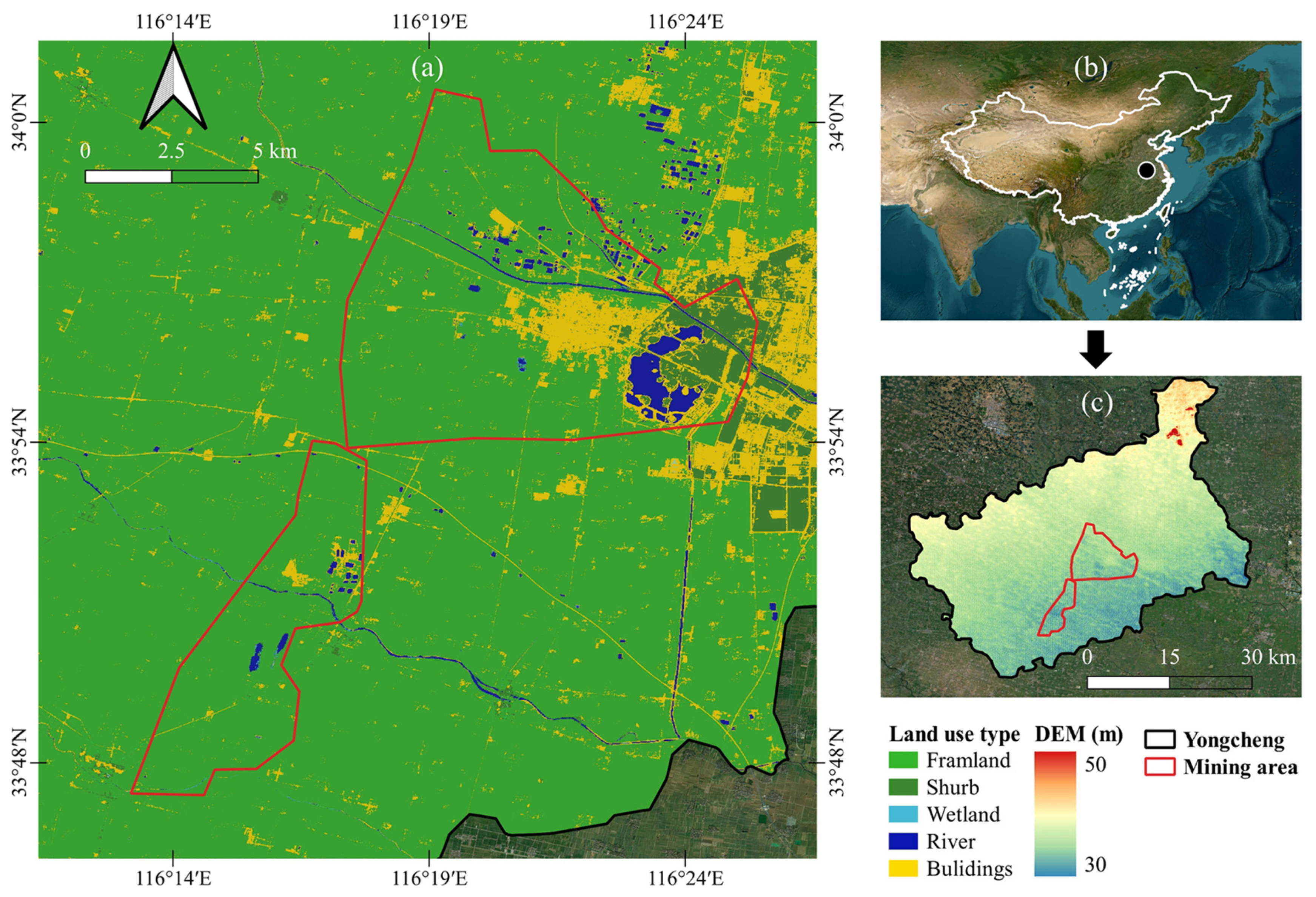
2.1. Overview of the Study Area

A junction between Henan, Jiangsu, and Anhui provinces, Yongcheng is located in the eastern section of Henan Province. It is situated where the Huanghuai Alluvial Plain and the North China Plain converge. Yongcheng has a lot of subsurface water sources and dense surface runoff due to its flat terrain (Figure 1c). There is a significant amount of farmed land (Figure 1a). It is a crucial grain base in China and one of the six key anthracite bases. The city of Yongcheng, which relies on energy resources, has actively supported local economic growth. Long-term coal mining has caused severe issues in the neighborhood.

After 2019, the local government in the research area decided to initiate land reclamation efforts with the intention of restoring agricultural production activities. They chose three waterlogged areas for different agricultural production modes, namely, a grain planting mode primarily focused on rice, a vegetable planting mode primarily centered around lotus, and a medicinal herb planting mode based on euryale.

2.2. Data Acquisition and Preprocessing

2.2.1. Remote Sensing Image Data Acquisition and Preprocessing

To categorize and track the development of crops planted in the subsidence area of the Yongcheng coal mining, we used Sentinel-1 and Sentinel-2 images. During the 2019–2022 crop growing season (May–October), we collect the monthly composite picture of the VV (vertical transmission and vertical reception) and VH (vertical transmission and horizontal reception) polarization of SAR–C (C-band) in IW (interferometric wideband mode) on the GEE (Google Earth Engine) platform. The GEE platform was used to gather Sentinel-2 images from the same period. The images were scaled to average reflectance after removing the clouds by dividing by 10,000. The images were finally synthesized for usage.

2.2.2. Sample Point Classification

We conducted a field survey in the study area in September 2022 and georeferenced the sample points there. The approximate location of sample points is shown in Figure 2.

When researchers went into the field, they discovered that some of the flooded farmland had been turned into an artificial wetland park. Due to the artificial wetland parks not being within the scope of this research, this part of the area has been excluded and referred to as engineering water. Visual interpretation was then added to the building sample points, natural water samples, and corn samples on the GEE platform. The sample points were randomly divided into training and verification sample points according to the ratio of 7:3, and the training sample set and the test sample set in the research area were obtained.

2.2.3. Crop Growth Period

Figure 3 shows the primary crops’ (euryale, rice, and lotus) growth and development stages. Although both lotus and euryale are members of the family Nymphaeaceae and develop similarly, they require distinct planting times and techniques. While lotus seeds may be planted outdoors in May, euryale seeds need to be started in a greenhouse or hotbed and given 30 to 40 days of growth before being put in paddy fields. Rice, like euryale, is raised from seed and transferred to a paddy field 20 to 30 days later, around the middle of May. Since rice and euryale seedling development is difficult to see because it occurs outside subsidence water areas, these two crops are monitored, starting in June. The primary crop grown in the study area throughout the summer is corn, which is typically sown at the end of May or the beginning of June and gradually develops from September to October.

3. Methods

This article utilizes machine learning classification methods to extract spatial distribution information of aquatic crops in the research area. Based on this, the article uses vegetation indices (VI) to monitor different crops’ growth and development curves during the 2022 growing season. According to the monitoring results, the best indices are selected for a comparative analysis of the growth conditions during the same period from 2019 to 2022. This section includes four subsections. Section 3.1.1 introduces the feature calculation and selection for crop classification in the research area. Section 3.1.2 introduces machine learning methods and precision evaluation criteria. Section 3.2 introduces two methods for analyzing crop growth conditions.

The steps are as follow: (1) Obtain the Sentinel image dataset from the GEE platform and carry out preprocessing operations; (2) The elevation features of the research region are corrected using MSPS before the features are built; (3) The classification of remote sensing images to extract the space distributing information of aquatic crops in the study area; (4) To create this box plot, we determine the maximum value, the upper and lower quartile values, the median value, and the average value of the optical vegetation index and polarization index of crops during their growth and development period; (5) The most stable optical VI are chosen, and the ratio is determined after taking into account the distribution of the index box plot and the difference between the median and average; (6) To evaluate the relative growth of various crops over the years, we calculate the ratio of their 2022 growth and development to their average growth and development across many years using the comparison approach. In Figure 4, the flow chart is displayed.

3.1. Remote Sensing Image Data Acquisition and Preprocessing

3.1.1. Classification Feature Calculation and Optimization

The original bands of the Sentinel-2 satellite contain a wealth of spectral information, making them suitable for inclusion as spectral features in classification.

Because various plants absorb or reflect the spectrum in slightly different ways, the index findings for different plants are not all the same. This allows for the differentiation of different vegetation types when using VI for qualitative and quantitative evaluations of vegetation cover and growth. The edge band has proven useful for monitoring vegetation’s physicochemical parameters in several previous studies [27,28,29]. Thus, the edge band for the red band and the estimated four planting cover indices (

Table 1. Index calculation formula.

Index	Formula
NDVI	$\left({\rho }_{NIR}-{\rho }_{RED}\right)/\left({\rho }_{NIR}+{\rho }_{RED}\right)$	(1)
NDVIed	$\left({\rho }_{NIR}-{\rho }_{RED-\mathrm{edge}5}\right)/\left({\rho }_{NIR}+{\rho }_{RED-\mathrm{edge}5}\right)$	(2)
EVI	$2.5\left({\rho }_{NIR}-{\rho }_{RED}\right)/\left({\rho }_{NIR}+6{\rho }_{RED}-7.5{\rho }_{BLUE}+1\right)$	(3)
EVIed	$2.5\left({\rho }_{NIR}-{\rho }_{RED-\mathrm{edge}5}\right)/\left({\rho }_{NIR}+6{\rho }_{RED-\mathrm{edge}5}-7.5{\rho }_{BLUE}+1\right)$	(4)
IBI	$\frac{2 {{\displaystyle \rho }}_{\mathrm{SWIR}1}/\left({{\displaystyle \rho }}_{\mathrm{SWIR}1}+{{\displaystyle \rho }}_{NIR}\right)-\left({{\displaystyle \rho }}_{NIR}/\left({{\displaystyle \rho }}_{RED}+{{\displaystyle \rho }}_{NIR}\right)+{{\displaystyle \rho }}_{\mathrm{GREEN}}/\left({{\displaystyle \rho }}_{\mathrm{GREEN}}+{{\displaystyle \rho }}_{\mathrm{SWIR}1}\right)\right)}{2 {{\displaystyle \rho }}_{\mathrm{SWIR}1}/\left({{\displaystyle \rho }}_{\mathrm{SWIR}1}+{{\displaystyle \rho }}_{NIR}\right)+\left({{\displaystyle \rho }}_{NIR}/\left({{\displaystyle \rho }}_{RED}+{{\displaystyle \rho }}_{NIR}\right)+{{\displaystyle \rho }}_{\mathrm{GREEN}}/\left({{\displaystyle \rho }}_{\mathrm{GREEN}}+{{\displaystyle \rho }}_{\mathrm{SWIR}1}\right)\right)}$	(5)
BSI	$\left(\left({{\displaystyle \rho }}_{SWIR1}+{\rho }_{RED}\right)-\left({\rho }_{NIR}+{\rho }_{BLUE}\right)\right)/\left(\left({{\displaystyle \rho }}_{SWIR1}+{\rho }_{RED}\right)+\left({\rho }_{NIR}+{\rho }_{BLUE}\right)\right)$	(6)
MNDWI	$\left({{\displaystyle \rho }}_{GREEN}-{{\displaystyle \rho }}_{SWIR1}\right)/\left({{\displaystyle \rho }}_{GREEN}+{{\displaystyle \rho }}_{SWIR1}\right)$	(7)
AWFI	$EVI<0.1, MNDWI>NDVI or MNDWI>EVI$	(8)
RVI	$4\ast VH/\left(VV+VH\right)$	(9)
Ratio	$VH/VV$	(10)

) are the Normalized Differential Vegetation Index (NDVI), the Enhanced Vegetation Index (EVI), the Normalized Differential Red-Edge Vegetation Index (NDVIed), and the Enhanced Red-Edge Vegetation Index (EVIed). The Annual Water Frequency Index (AWFI) [30] can identify seasonal waterlogging caused by mining subsidence, help improve the classification accuracy of aquatic crops in subsidence water areas, and, together with the Modified Normalized Differential Water Index (MNDWI), constitute water feature parameters. The Index-based Built-up Index (IBI) and Bare Soil Index (BSI) are introduced for large building land in mining areas. Together, these indices form the Index feature.

The classification impact will be influenced by the phenomena of “same thing with different spectrum and foreign item with the same spectrum”, even if the spectral index may distinguish vegetation, water bodies, buildings, etc. Researchers [31,32] have attempted to calculate texture features to supplement the spectral information to improve classification accuracy and better distinguish between different ground objects. Therefore, this study selected six commonly used texture indices (Contrast, Variance, Entropy, Inverse Difference Moment, Angular Second Moment, and Correlation) to be included as texture features in the classification.

Shadow effects of images (changes in light conditions caused by topography or tall buildings and clouds) affect another aspect of feature classification. Due to the different optical sensor and SAR imaging mechanisms, a large amount of complementary information can be obtained when optical and SAR data are used simultaneously, which is crucial in improving classification accuracy. More information is gained that is helpful in classifying and recognizing ground objects when optical and SAR data are utilized together. Therefore, in this study, VV, VH, VH/VV Ratio, and Radar Vegetation Index (RVI) are used as polarimetric features for classification.

SRTM DEM data cannot capture the collapsed basin resulting from ground subsidence from coal mining. As a result, this study, using the probability integral method and the measured surface movement parameters in the mining area, along with mining practice and the mechanical and physical properties of the overburdened rock, identified the mining working face in the mining area and predicted the surface movement, using this software for predicting mining subsidence (MSPS). Therefore, this study included the corrected DEM data as elevation features in the classification.

3.1.2. Machine Learning Classification Method

The selection of feature variables is a crucial step in remote sensing classification. Combining various feature variables can effectively improve the accuracy of remote sensing classification. However, an excessive number of feature variables can reduce the accuracy of classification results. Therefore, it is necessary to filter the features before classification. In this study, the RF classifier is used to assess the importance of features through the Gini Coefficient, which facilitates feature selection. The importance score values from 10 iterations of classification are collected and averaged. Features with score values below the average are excluded from the classification.

In addition to the RF classifier, this study also utilized the commonly used SVM classifier and the Classification and Regression Trees (CART) classifier [33]. All three of these classifiers require parameter tuning to achieve the best performance. After multiple attempts, RF classifiers determined that setting the number of decision trees to 25 yielded the best classification results. SVM classifiers are effective at handling non-linear classification problems, especially when using the LINEAR kernel function. The maximum number of nodes in each decision tree is an important parameter for CART classifiers and was set to 35 in this experiment.

As described in Section 2.2.2, the sample points are randomly divided in a 7:3 ratio, resulting in different outcomes each time the classification is performed. To reduce the impact of random training sample selection on classification accuracy, in this experiment, the overall accuracy (OA) and average Kappa coefficient for each classifier were computed by averaging the results of 10 iterations.

In this study, classification features are added step by step. Initially, optical features, index features, and original DEM data are added, and the classification results are named RF1, SVM1, and CART1. Subsequently, modified DEM data are used to replace the original DEM data, and the classification results are named RF2, SVM2, and CART2. Finally, all the features are included, and the classification results are named RF3, SVM3, and CART3.

3.2. Assessing the Development and Growth of Crops

Crop growth conditions refer to the state and trends of crop growth. Different types of crops, and even the same type of crop grown in different environments, can exhibit different growth characteristics. Therefore, it is scientifically meaningful to compare crop growth conditions using a standardized method to ensure consistency in the results. The three primary techniques for crop growth monitoring are direct observation, comparative assessment, and following the growth process.

The direct observation method refers to the construction of empirical models using remote sensing techniques and statistical models to obtain agronomic indicators closely related to crop growth, such as leaf area and crop biomass. This method is not only convenient and fast but also accurate. However, it lacks scientific significance when comparing different crops due to significant differences in agronomic indicators among various crops.

Following the growth process method and the comparative assessment method can reduce the impact of crop types and enable a standardized comparison across different crops. Therefore, this study utilizes both methods to compare the growth conditions of crops in the subsidence areas.

Following the growth process method mainly adopts the average VI time series curve change in the current year for analysis [34]. This approach does not take into account the impact of the crop itself, and instead acts on the vegetation-specific spectral features. In this study, an index box plot has been added on this basis to enrich growth information and compare monitoring results. A box plot is composed of the minimum value, upper and lower quartiles, and median. The box, which is the region between the two quartiles, represents 50% of the data. The length of the box reflects the stability of the data and indicates the tendency of the data to be concentrated or dispersed. A flatter box indicates that the data have less variation, meaning it is more stable.

The comparative assessment method primarily compares the index of the current year with the same index of the previous year, the average of many years, or the same index of a specified year to reflect the difference in crop growth status between the years. The comparison is shown in Formula (11).

$$D_i=\frac{V{I}_{2022}-\overline{V{I}_i}}{\overline{V{I}_i}}$$

(11)

$V{I}_{2022}$ is the average of 2022 data $\overline{V{I}_i}$ and represents the data average from 2019 to 2022. The comparison ($D_i$) findings are on a scale of −1 to 1, where a positive result indicates increased growth over previous years and a negative result indicates decreased growth. These findings are then divided into eight categories using intervals of 0.25, namely, slight growth, mild growth, moderate growth, significant growth, slight decline, mild decline, moderate decline, and significant decline.

Currently, many kinds of spectral vegetation indices are used for growth monitoring, among which NDVI and EVI are widely used [35,36,37]. Similarly, to the issues encountered in the vegetation classification in Section 3.1, cloud cover and shadow effects in the research area can also affect the monitoring effectiveness of NDVI and EVI. Due to the unique mode of action and the capabilities of radar remote sensing data for all-weather monitoring, researchers also use polarization indicators (VV, VH, VH/VV Ratio, RVI) for growth monitoring [38,39,40].

4. Results

4.1. Crop Classification Results in Subsidence Areas

As shown in Figure 5b–d, using DEM with subsidence contour lines can provide a more detailed representation of subsidence topography. Using this as a classification feature should help improve the classification performance of crops. This high-resolution terrain information can offer more insights into surface changes, enhancing the accuracy and performance of the classification model.

The classification feature importance calculated through the RF model is shown in Figure 6. The mean score was the limit to eliminate the feature variables with low scores. The polarization property is ranked second in importance to DEM in Figure 6.

As shown in

Table 2. Classification accuracy before and after DEM modification.

	Corn	Buildings	River	Engineering Water	Lotus	Euryale	Rice	OA	Kappa
RF1	0.98	0.92	0.91	0.74	0.66	0.40	0.75	0.83	0.82
RF2	0.97	0.93	0.90	0.79	0.85	0.72	0.80	0.90	0.87
RF3	0.99	0.97	0.92	0.79	0.85	0.77	0.79	0.92	0.90
SVM1	0.98	0.94	0.71	0.58	0.64	0.26	0.61	0.70	0.61
SVM2	0.98	0.93	0.70	0.69	0.85	0.38	0.81	0.80	0.74
SVM3	0.98	0.94	0.86	0.62	0.82	0.60	0.74	0.87	0.83
CART1	0.86	0.84	0.74	0.65	0.53	0.57	0.65	0.78	0.72
CART2	0.95	0.89	0.80	0.73	0.79	0.62	0.76	0.85	0.81
CART3	0.96	0.93	0.83	0.78	0.86	0.65	0.77	0.87	0.84

, the corrected DEM data significantly improved the classification results, leading to an average increase of 7.77% in overall accuracy and a 9.06% improvement in the Kappa coefficient. The corrected DEM data also enhanced the classification accuracy of lotus, euryale, and rice, resulting in an average improvement of 22.01%, 16.42%, and 11.95%, respectively. The corrected DEM data (Figure 5) highlighted the location of coal mining subsidence areas, combined with different spectral indices emphasizing water body and vegetation information. This approach led to high classification accuracy for lotus and rice (average accuracy of 0.83 and 0.79, respectively) but poor accuracy for euryale (average accuracy of 0.57). Further classification features need to be added to improve the accuracy for euryale.

The inclusion of texture and polarization features significantly improved the classification of Euryale, resulting in an average accuracy improvement of 14.45%. Among the three machine learning methods, Random Forest classification (RF3) achieved the highest accuracy, with an overall accuracy of 92.39% and a Kappa coefficient of 0.90. The classification results after adding texture and polarization features are depicted in Figure 7.

Part of the rice planting area was incorrectly categorized as lotus, as indicated in the rice classification results for the three classification techniques Figure 7(a1–a3). CART3 achieved a relatively high classification accuracy for rice with a value of 0.78. However, Figure 7(a3) shows that it had the largest misclassification area. SVM3 had the lowest classification accuracy for rice, with a score of 0.74, while RF3 had the highest accuracy for rice, reaching 0.79.

The coal mining subsidence areas where euryale is located are close to the village. Due to the land subsidence, the road that originally separated the village from the farmland is now submerged, making it difficult to define the edges of the planting area. Additionally, due to factors like the planting density of euryale, some areas within the planting zone are misclassified as water Figure 7(b1–b3). Figure 7 shows that lotus has the most accurate classification of all aquatic crops. It is crucial to note that while Figure 7(c3) incorrectly classified certain lotus as rivers, Figure 7(c1,c2) performed well in categorization.

The local government in the study area transformed the eastern coal mining subsidence water area into wetland parks and the central coal mining subsidence water area into plain reservoirs (as shown in Figure 7d). RF3, with an accuracy of 0.79, and CART3, with an accuracy of 0.78, performed well in the classification and recognition of engineering water.

Based on the analysis presented, the RF method successfully identified all three types of aquatic crops with minimal errors. As a result, the classification accuracy of RF3, which had the highest accuracy, was chosen as the final classification result for further growth analysis. The rice, euryale, and lotus planting areas in the research region were 95.5 ha, 221.1 ha, and 208.9 ha, respectively. Figure 7a demonstrates that rice predominates in the center of the study area. Euryale is primarily found in the northwest region (as depicted in Figure 7b). Lotus is primarily found in the southern region (as illustrated in Figure 7c). Engineering water is present in the middle portion of the research region (as seen in Figure 7d).

4.2. Growth Monitoring Results

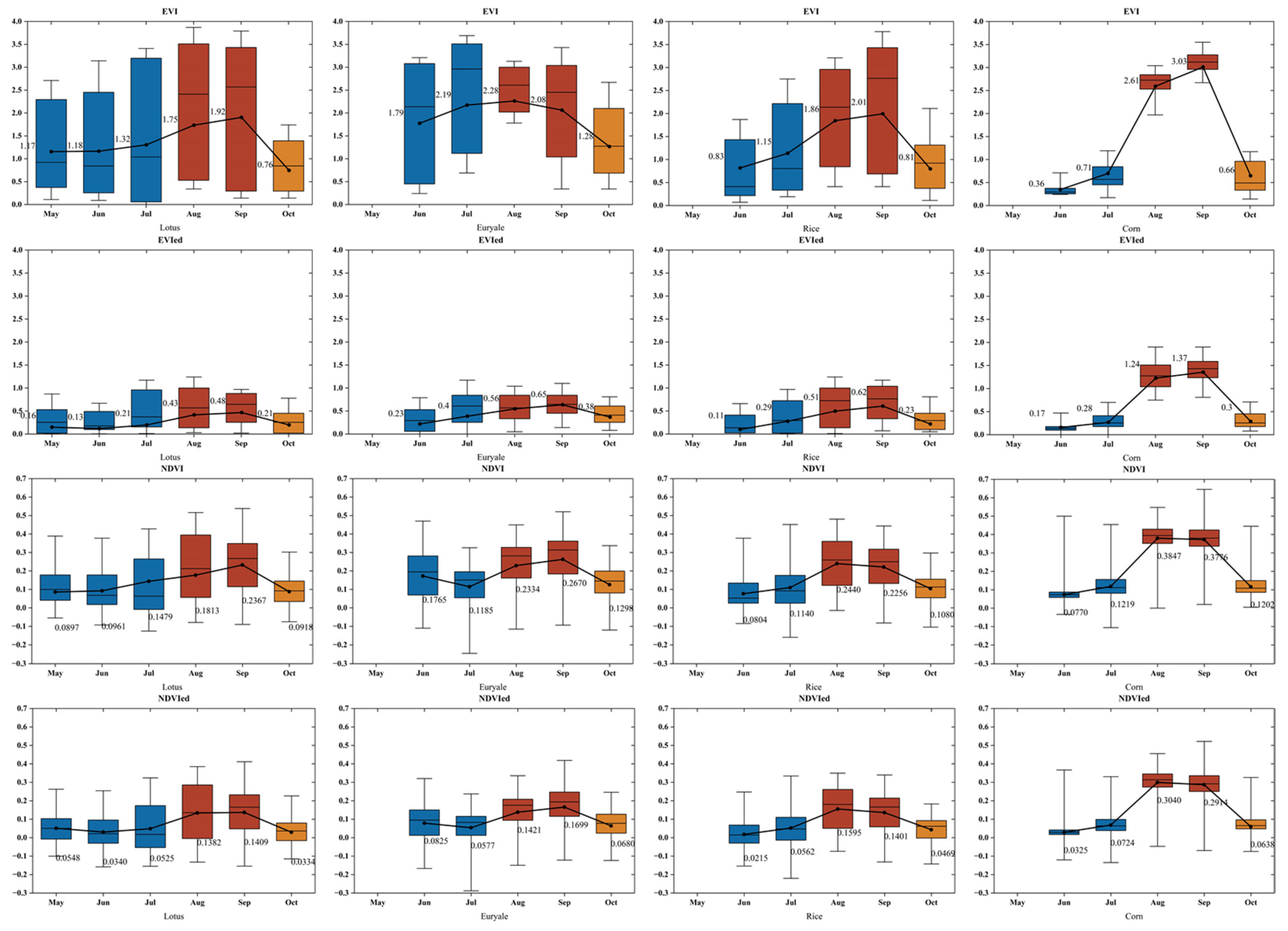
4.2.1. Monitoring of Crop Growth Process

Different crops and different indices show bell-shaped curves with an initial increase and subsequent decrease, but the curvature, peak values, and timing of peak occurrences vary based on crop varieties and the monitored indices.

In the early growth stages, from May to July, crops primarily grow vertically, and the plant distribution is sparse. Therefore, crop volume scattering plays a minor role in total backscattering, while ground background scattering (soil surface scattering and water surface specular reflection) dominates. Different crops and different indices show bell-shaped curves with an initial increase and subsequent decrease, but the curvature, peak values, and timing of peak occurrences vary based on crop varieties and the monitored indices. In the early growth stages, from May to July, crops primarily grow vertically, and the plant distribution is sparse. Therefore, crop volume scattering plays a minor role in total backscattering, while ground background scattering dominates.

RVI mainly captures the volume scattering of plants and is more representative of the early growth and development of crops relative to the other three polarimetric features. As shown in Figure 8, the RVI box plot curve demonstrates that during the early growth stages, RVI values continuously increase and reach their peak in July, with lotus reaching its peak value at 2.483 and an average growth rate of 3.5%, euryale reaching its peak value at 2.590 with an average growth rate of 2.3%, rice achieving its peak value at 2.595 with an average growth rate of 4.2%, and corn reaching its peak value at 2.535 with an average growth rate of 4.0%.

From July to August, plants start to grow leaves and canopy structures, reaching maximum density in September. During this period, the crops have robust branches and leaves, with a dense canopy that blocks ground background scattering, resulting in lower index values. September to October represents the maturation period for crops. As the fruits mature, the plants’ water content significantly decreases, causing them to turn yellow. During this phase, ground background scattering becomes dominant.

Some of the spectral index monitoring results appear contradictory to the actual growth process. For instance, as shown in Figure 9, the NDVI and NDVIed values exhibit a decrease during the growth phases of euryale in June to July and lotus in May to June. This discrepancy contradicts the expected vigorous vegetation growth, indicating a noticeable error.

During July to September, when vegetation coverage is high, the spectral index monitoring results are more in line with the actual situation. Because the NDVIed monitoring values exhibit the most stable box plot curve and align most closely with a normal distribution (i.e., the mean is closest to the median), they are used for growth monitoring. Lotus reached its peak value in September (0.140), with an average growth rate of 82.6%. Euryale reached its peak value in September (0.170), with an average growth rate of 82.9%. Rice reached its peak value in August (0.160), with an average growth rate of 183.8%. Corn reached its peak value in August (0.304), with an average growth rate of 319.9%. Combining these two sets of data, it is clear that corn has the highest growth rate and the highest peak value, indicating that corn’s growth is best during the mid-growth stage.

From this, it can be seen that the reclamation results of the three agricultural reclamation models have not yet met the local agricultural average standards. There is still considerable room for improvement in these three agricultural reclamation models.

4.2.2. Comparison of Crop Growth in the Same Period

Considering that using different indices can impact the comparison of growth trends in the same period and in accordance with the content of Section 3.2, RVI is used for comparing growth trends from June to July (with the monitoring of lotus starting from May), as shown in Figure 10. From August to September, NDVIed is used for comparison, as depicted in Figure 11. Due to the different harvest times of crops in the late growth period (October), comparisons for October are conducted.

In the early growth period, the entire mining area’s comparative results for the same period (Figure 10a) fall within the range of slight decline to slight growth, i.e., [−0.25, 0.25]. The area with slight growth in vegetation covers 56.78% of the total area. From June to July 2022, 56.78% of the region showed better growth conditions compared to the average level from 2019 to 2022. Figure 10b–e represent the growth trends of rice, euryale, lotus, and corn in the early growth period from 2019 to 2022. The pie charts illustrate the proportion of each crop’s growth categories: the area with slight growth, ranked from largest to smallest, is rice (70.2%), euryale (65.6%), lotus (60.1%), and corn (56.4%).

During the mid-growth stage, the study area as a whole experienced a slight decline in overall growth, covering 95.99% of the total area (Figure 11a). This indicates that, in September 2022, 95.99% of the region had growth conditions worse than the 2019–2022 average. Figure 11b–e represent the comparative results of the mid-growth stage for rice, euryale, lotus, and corn in the years 2019–2022. This offers a more intuitive comparison than the early growth stage, particularly concerning the different growth levels of the three aquatic crops. Specifically, rice had an overall growth area of 47.4%, with a significant growth area of 12.1%; euryale’s overall growth area was 43.4%, with a significant growth area of 15.3%; and lotus had an overall growth area of 27.6%, with a significant growth area of 2.4%.

In the early growth stage, both aquatic and corn reached an average level of growth and development in most regions, similarly to previous years. During the mid-growth stage, considering the entire mining area, the growth situation in 2022 as a whole was generally worse than the 2019–2022 average. However, when looking at different crops, the growth conditions of the three aquatic crops were better than the overall mining area, indicating that the growth in 2022 was superior to the average level. Therefore, it can be concluded that the reclamation effectiveness of these three agricultural reclamation models is gradually improving.

5. Discussion

5.1. The Relationship between S1 and S2 Parameters and Crop Growth and Development

This study is based on Sentinel satellite data to monitor the crop growth situation in coal mining subsidence water areas and evaluate the effectiveness of local agricultural reclamation work through peak vegetation index data during the growing season and multi-year comparative results.

When vegetation coverage is low, particularly during the early growth stages and after harvest, the spectral reflectance from the soil or water background dominates the monitoring results of NDVI and NDVIed [41,42]. EVI provides poor monitoring outcomes for aquatic crops despite its ability to lessen the impact of soil background by tweaks to soil parameters [43]. Overall, optical vegetation indices struggle to simultaneously remove the interference from water and ground backgrounds, leading to some degree of error in the monitoring results.

Similarly, to the spectral index, the radar signal also contains soil and water background. Studies have shown that the ratio and RVI weaken this part of the impact, that is, the ratio and RVI mainly receive the volume scattering signal of the plant itself and the double rebound scattering signal of the plant canopy with the wet soil or water surface [26,39]. In the early stages of crop growth, the vegetation canopy has not fully developed, resulting in relatively fewer double bounce scattering signals between plants and moist soil or water surfaces.

During the mid-growth stage of crops, plant stems and leaves grow vigorously, and the vegetation canopy covers the entire ground or water surface. At this time, ground reflection signals are obscured by the canopy, and the received radar signals primarily consist of volume scattering signals from the plant canopy. The received optical reflection signals originate from the canopy reflection. The volume scattering signal from the plant canopy is mainly related to the complexity of the canopy structure, which might vary for different crop types and could influence the results.

In the early stages of crop growth and development, when the vegetation cover is low, radar indices can, to some extent, replace optical vegetation indices in monitoring the crop’s growth status.

5.2. Common Reclamation Measures of Coal Mining Subsidence Water Areas

The treatment of coal mining subsidence has always been the research focus of land reclamation and ecological restoration in the coal mining area. In terms of reclamation technology of coal subsidence, non-filling reclamation methods such as the drainage method, deep digging and shallow pad method, and mud pump method were initially proposed, as well as filling reclamation technology using coal gangue, fly ash, and Yellow River sediment [44,45] as filling materials. In addition to coupled aboveground and underground land reclamation technologies [46], significant progress has been made. However, in the eastern high groundwater level coal mining subsidence areas, the subsidence basins are extensive and voluminous, requiring a significant amount of materials for backfill reclamation [47]. Traditional land reclamation methods are not feasible in this context. Therefore, in this area, various remediation techniques such as water purification, water system connectivity, substrate modification, plant restoration, and landscape design are primarily employed to transform the coal mining subsidence waterlogged areas into wetland ecosystems with landscape ecological significance. These areas are developed as artificial wetland parks, aquaculture zones, reservoirs, and water storage ponds, among others [48,49,50], such as the Xuzhou Pan’an Lake Wetland Park and the Huainan Lu Jin Lake Wetland Park.

The delicate balancing act between mining and protected farmland is important in the heavily populated eastern plains. Based on this real-world issue, the local government chose to develop and utilize coal mining subsidence water areas for agriculture rather than transforming them into artificial wetlands. Agricultural reclamation in these waterlogged areas helps maintain local food stability and mitigate conflicts between people and land, resulting in significant social benefits.

5.3. Recommendations

Due to the lack of familiarity among staff with land reclamation and agricultural engineering management, there are still certain issues in the local work. Here are the recommendations based on this study:

• The reclamation results for the vegetable planting mode primarily centered around lotus have not been ideal, both spatially and temporally. The local area should reduce the application of this mode gradually.
• Control the area dedicated to the grain planting mode primarily focused on rice. While rice cultivation depends on water, the fields need to be kept dry before harvest. Waterlogged areas with significant subsidence depths may struggle to meet the necessary growth conditions for rice.

6. Conclusions

This study utilized machine learning methods to obtain the spatial distribution of three aquatic crops (lotus, rice, and euryale) and the major local crop, corn, in coal mining subsidence water areas. This research also involved monitoring the growth processes and conducting concurrent assessments of their growth trends. The results of the study indicate that:

• The accuracy of classifying aquatic crops, such as lotus, euryale, and rice, improved by 22.01%, 16.42%, and 11.95%, respectively, after using the mining area elevation information rectified by the MSPS.
• The Random Forest classifier using a combination of optical features, spectral features, elevation features, texture features, and polarization features achieved the best crop classification results for the study area, with an overall accuracy of 92.39% and a Kappa coefficient of 0.90.
• The peak RVI values for crops from May to July were ranked in the following order: rice (2.595), euryale (2.590), corn (2.535), and lotus (2.483). During the period from August to September, the peak NDVIed values followed this ranking: corn (0.304), euryale (0.170), rice (0.160), and lotus (0.140).
• The order of crops showing improved growth conditions during the early growth stage was as follows: rice (70.2%), euryale (65.6%), lotus (60.1%), and corn (56.4%). During the mid-growth stage, it followed this sequence: rice (47.4%), euryale (43.4%), lotus (27.6%), and corn (4.01%).

This study describes the agricultural reclamation outcomes in coal mining subsidence water areas through the growth and development of crops. It provides valuable insights into local agricultural management and land reclamation efforts.

References

1. Guzy, A.; Malinowska, A.A. Assessment of the Impact of the Spatial Extent of Land Subsidence and Aquifer System Drainage Induced by Underground Mining. Sustainability 2020, 12, 7871. [Google Scholar] [CrossRef]
2. Akcin, H.; Kutoglu, H.S.; Kemaldere, H.; Deguchi, T.; Koksal, E. Monitoring subsidence effects in the urban area of Zonguldak Hardcoal Basin of Turkey by InSAR-GIS integration. Nat. Hazards Earth Syst. Sci. 2010, 10, 1807–1814. [Google Scholar] [CrossRef]
3. Solarski, M.; Machowski, R.; Rzetala, M.; Rzetala, M.A. Hypsometric changes in urban areas resulting from multiple years of mining activity. Sci. Rep. 2022, 12, 2982. [Google Scholar] [CrossRef] [PubMed]
4. Wang, J.; Wang, P.; Qin, Q.; Wang, H. The effects of land subsidence and rehabilitation on soil hydraulic properties in a mining area in the Loess Plateau of China. CATENA 2017, 159, 51–59. [Google Scholar] [CrossRef]
5. Fan, T.-Y.; Yan, J.-P.; Wang, S.; Zhang, B.; Ruan, S.-X.; Zhang, M.-L.; Li, S.-Q.; Chen, Y.-C.; Liu, J. Water quality variation of mining-subsidence lake during the initial stage: Cases study of Zhangji and Guqiao Mines. J. Coal Sci. Eng. 2012, 18, 297–301. [Google Scholar] [CrossRef]
6. Cheng, W.; Bian, Z.-F.; Dong, J.-H.; Lei, S.-G. Soil properties in reclaimed farmland by filling subsidence basin due to underground coal mining with mineral wastes in China. Trans. Nonferrous Met. Soc. 2014, 24, 2627–2635. [Google Scholar] [CrossRef]
7. Zhang, H.; Yan, Q.; Xie, F.; Ma, S. Evaluation and Prediction of Landscape Ecological Security Based on a CA-Markov Model in Overlapped Area of Crop and Coal Production. Land 2023, 12, 207. [Google Scholar] [CrossRef]
8. Xiao, W.; Zheng, W.; Zhao, Y.; Chen, J.; Hu, Z. Examining the relationship between coal mining subsidence and crop failure in plains with a high underground water table. J. Soils Sediments 2021, 21, 2908–2921. [Google Scholar] [CrossRef]
9. Ren, H.; Xiao, W.; Zhao, Y.; Hu, Z. Land damage assessment using maize aboveground biomass estimated from unmanned aerial vehicle in high groundwater level regions affected by underground coal mining. Environ. Sci. Pollut. Res. 2020, 27, 21666–21679. [Google Scholar] [CrossRef]
10. Xiong, J.; Thenkabail, P.S.; Tilton, J.C.; Gumma, M.K.; Teluguntla, P.; Oliphant, A.; Congalton, R.G.; Yadav, K.; Gorelick, N. Nominal 30-m Cropland Extent Map of Continental Africa by Integrating Pixel-Based and Object-Based Algorithms Using Sentinel-2 and Landsat-8 Data on Google Earth Engine. Remote Sens. 2017, 9, 1065. [Google Scholar] [CrossRef]
11. Zhang, P.; Hu, S.; Li, W.; Zhang, C. Parcel-level mapping of crops in a smallholder agricultural area: A case of central China using single-temporal VHSR imagery. Comput. Electron. Agric. 2020, 175, 105581. [Google Scholar] [CrossRef]
12. Gao, F.; Anderson, M.C.; Zhang, X.; Yang, Z.; Alfieri, J.G.; Kustas, W.P.; Mueller, R.; Johnson, D.M.; Prueger, J.H. Toward mapping crop progress at field scales through fusion of Landsat and MODIS imagery. Remote Sens. Environ. 2017, 188, 9–25. [Google Scholar] [CrossRef]
13. Magney, T.S.; Eitel, J.U.; Huggins, D.R.; Vierling, L.A. Proximal NDVI derived phenology improves in-season predictions of wheat quantity and quality. Agric. For. Meteorol. 2016, 217, 46–60. [Google Scholar] [CrossRef]
14. Zheng, H.; Cheng, T.; Yao, X.; Deng, X.; Tian, Y.; Cao, W.; Zhu, Y. Detection of rice phenology through time series analysis of ground-based spectral index data. Field Crops Res. 2016, 198, 131–139. [Google Scholar] [CrossRef]
15. Ge, Y.; Bai, G.; Stoerger, V.; Schnable, J.C. Temporal dynamics of maize plant growth, water use, and leaf water content using automated high throughput RGB and hyperspectral imaging. Comput. Electron. Agric. 2016, 127, 625–632. [Google Scholar] [CrossRef]
16. Dong, T.; Liu, J.; Qian, B.; Zhao, T.; Jing, Q.; Geng, X.; Wang, J.; Huffman, T.; Shang, J. Estimating winter wheat biomass by assimilating leaf area index derived from fusion of Landsat-8 and MODIS data. Int. J. Appl. Earth Obs. Geoinf. 2016, 49, 63–74. [Google Scholar] [CrossRef]
17. Huang, J.; Tian, L.; Liang, S.; Ma, H.; Becker-Reshef, I.; Huang, Y.; Su, W.; Zhang, X.; Zhu, D.; Wu, W. Improving winter wheat yield estimation by assimilation of the leaf area index from Landsat TM and MODIS data into the WOFOST model. Agric. For. Meteorol. 2015, 204, 106–121. [Google Scholar] [CrossRef]
18. Liang, L.; Di, L.; Zhang, L.; Deng, M.; Qin, Z.; Zhao, S.; Lin, H. Estimation of crop LAI using hyperspectral vegetation indices and a hybrid inversion method. Remote Sens. Environ. 2015, 165, 123–134. [Google Scholar] [CrossRef]
19. Yuan, H.; Yang, G.; Li, C.; Wang, Y.; Liu, J.; Yu, H.; Feng, H.; Xu, B.; Zhao, X.; Yang, X. Retrieving Soybean Leaf Area Index from Unmanned Aerial Vehicle Hyperspectral Remote Sensing: Analysis of RF, ANN, and SVM Regression Models. Remote Sens. 2017, 9, 309. [Google Scholar] [CrossRef]
20. Yue, J.; Yang, G.; Li, C.; Li, Z.; Wang, Y.; Feng, H.; Xu, B. Estimation of Winter Wheat Above-Ground Biomass Using Unmanned Aerial Vehicle-Based Snapshot Hyperspectral Sensor and Crop Height Improved Models. Remote Sens. 2017, 9, 708. [Google Scholar] [CrossRef]
21. Li, W.; Niu, Z.; Chen, H.; Li, D.; Wu, M.; Zhao, W. Remote estimation of canopy height and aboveground biomass of maize using high-resolution stereo images from a low-cost unmanned aerial vehicle system. Ecol. Indic. 2016, 67, 637–648. [Google Scholar] [CrossRef]
22. Cai, Y.; Guan, K.; Lobell, D.; Potgieter, A.B.; Wang, S.; Peng, J.; Xu, T.; Asseng, S.; Zhang, Y.; You, L.; et al. Integrating satellite and climate data to predict wheat yield in Australia using machine learning approaches. Agric. For. Meteorol. 2019, 274, 144–159. [Google Scholar] [CrossRef]
23. Lizaso, J.I.; Ruiz-Ramos, M.; Rodríguez, L.; Gabaldon-Leal, C.; Oliveira, J.A.; Lorite, I.J.; Sánchez, D.; García, E.; Rodríguez, A. Impact of high temperatures in maize: Phenology and yield components. Field Crops Res. 2018, 216, 129–140. [Google Scholar] [CrossRef]
24. Zhou, X.; Zheng, H.B.; Xu, X.Q.; He, J.Y.; Ge, X.K.; Yao, X.; Cheng, T.; Zhu, Y.; Cao, W.X.; Tian, Y.C. Predicting grain yield in rice using multi-temporal vegetation indices from UAV-based multispectral and digital imagery. ISPRS J. Photogramm. Remote Sens. 2017, 130, 246–255. [Google Scholar] [CrossRef]
25. Liu, C.-A.; Chen, Z.-X.; Shao, Y.; Chen, J.-S.; Hasi, T.; Pan, H.-Z. Research advances of SAR remote sensing for agriculture applications: A review. J. Integr. Agric. 2019, 18, 506–525. [Google Scholar] [CrossRef]
26. Khabbazan, S.; Vermunt, P.; Steele-Dunne, S.; Arntz, L.R.; Marinetti, C.; van der Valk, D.; Iannini, L.; Molijn, R.; Westerdijk, K.; van der Sande, C. Crop Monitoring Using Sentinel-1 Data: A Case Study from The Netherlands. Remote Sens. 2019, 11, 1887. [Google Scholar] [CrossRef]
27. Xie, Q.; Dash, J.; Huang, W.; Peng, D.; Qin, Q.; Mortimer, H.; Casa, R.; Pignatti, S.; Laneve, G.; Pascucci, S.; et al. Vegetation Indices Combining the Red and Red-Edge Spectral Information for Leaf Area Index Retrieval. IEEE J. Sel. Top. Appl. Earth Obs. Remote Sens. 2018, 11, 1482–1493. [Google Scholar] [CrossRef]
28. Fernández-Manso, A.; Fernández-Manso, O.; Quintano, C. SENTINEL-2A red-edge spectral indices suitability for discriminating burn severity. Int. J. Appl. Earth Obs. Geoinf. 2016, 50, 170–175. [Google Scholar] [CrossRef]
29. Kanke, Y.; Tubaña, B.; Dalen, M.; Harrell, D. Evaluation of red and red-edge reflectance-based vegetation indices for rice biomass and grain yield prediction models in paddy fields. Precis. Agric. 2016, 17, 507–530. [Google Scholar] [CrossRef]
30. He, T.; Xiao, W.; Zhao, Y.; Chen, W.; Deng, X.; Zhang, J. Continues monitoring of subsidence water in mining area from the eastern plain in China from 1986 to 2018 using Landsat imagery and Google Earth Engine. J. Clean. Prod. 2021, 279, 123610. [Google Scholar] [CrossRef]
31. Xu, X.; Li, Y.; Wu, Q.J. A compact multi-pattern encoding descriptor for texture classification. Digit. Signal Process. 2021, 114, 103081. [Google Scholar] [CrossRef]
32. Xu, Y.; Zhang, S.; Li, J.; Liu, H.; Zhu, H. Extracting Terrain Texture Features for Landform Classification Using Wavelet Decomposition. ISPRS Int. J. Geo-Inf. 2021, 10, 658. [Google Scholar] [CrossRef]
33. Tamiminia, H.; Salehi, B.; Mahdianpari, M.; Quackenbush, L.; Adeli, S.; Brisco, B. Google Earth Engine for geo-big data applications: A meta-analysis and systematic review. ISPRS J. Photogramm. Remote Sens. 2020, 164, 152–170. [Google Scholar] [CrossRef]
34. Alam Shammi, S.; Meng, Q. Use time series NDVI and EVI to develop dynamic crop growth metrics for yield modeling. Ecol. Indic. 2021, 121, 107124. [Google Scholar] [CrossRef]
35. Atzberger, C. Advances in Remote Sensing of Agriculture: Context Description, Existing Operational Monitoring Systems and Major Information Needs. Remote Sens. 2013, 5, 949–981. [Google Scholar] [CrossRef]
36. Glenn, E.P.; Huete, A.R.; Nagler, P.L.; Nelson, S.G. Relationship between remotely-sensed vegetation indices, canopy attributes and plant physiological processes: What vegetation indices can and cannot tell us about the landscape. Sensors 2008, 8, 2136–2160. [Google Scholar] [CrossRef]
37. Pettorelli, N.; Vik, J.O.; Mysterud, A.; Gaillard, J.-M.; Tucker, C.J.; Stenseth, N.C. Using the satellite-derived NDVI to assess ecological responses to environmental change. Trends Ecol. Evol. 2005, 20, 503–510. [Google Scholar] [CrossRef]
38. Kim, Y.; Jackson, T.; Bindlish, R.; Hong, S.; Jung, G.; Lee, K. Retrieval of Wheat Growth Parameters with Radar Vegetation Indices. IEEE Geosci. Remote Sens. Lett. 2014, 11, 808–812. [Google Scholar] [CrossRef]
39. Kim, Y.; Jackson, T.; Bindlish, R.; Lee, H.; Hong, S. Radar Vegetation Index for Estimating the Vegetation Water Content of Rice and Soybean. IEEE Geosci. Remote Sens. Lett. 2012, 9, 564–568. [Google Scholar] [CrossRef]
40. Szigarski, C.; Jagdhuber, T.; Baur, M.; Thiel, C.; Parrens, M.; Wigneron, J.-P.; Piles, M.; Entekhabi, D. Analysis of the Radar Vegetation Index and Potential Improvements. Remote Sens. 2018, 10, 1776. [Google Scholar] [CrossRef]
41. Wang, M.; Luo, Y.; Zhang, Z.; Xie, Q.; Wu, X.; Ma, X. Recent advances in remote sensing of vegetation phenology: Retrieval algorithm and validation strategy. Natl. Remote Sens. Bull. 2022, 26, 431–455. [Google Scholar] [CrossRef]
42. Huete, A.R. A soil-adjusted vegetation index (SAVI). Remote Sens. Environ. 1988, 25, 295–309. [Google Scholar] [CrossRef]
43. Huete, A.; Justice, C.; Liu, H. Development of vegetation and soil indices for MODIS-EOS. Remote Sens. Environ. 1994, 49, 224–234. [Google Scholar] [CrossRef]
44. Hu, Z.; Wang, X.; McSweeney, K.; Li, Y. Restoring subsided coal mined land to farmland using optimized placement of Yellow River sediment to amend soil. Land Degrad. Dev. 2022, 33, 1029–1042. [Google Scholar] [CrossRef]
45. Wang, P.; Hu, Z.; Yost, R.S.; Shao, F.; Liu, J.; Li, X. Assessment of chemical properties of reclaimed subsidence land by the integrated technology using Yellow River sediment in Jining, China. Environ. Earth Sci. 2016, 75, 1046. [Google Scholar] [CrossRef]
46. Li, G.; Hu, Z.; Li, P.; Yuan, D.; Feng, Z.; Wang, W.; Fu, Y. Innovation for sustainable mining: Integrated planning of underground coal mining and mine reclamation. J. Clean. Prod. 2022, 351, 131522. [Google Scholar] [CrossRef]
47. Feng, Z.; Hu, Z.; Li, G.; Zhang, Y.; Zhang, X.; Zhang, H. Improving mine reclamation efficiency for farmland sustainable use: Insights from optimizing mining scheme. J. Clean. Prod. 2022, 379, 134615. [Google Scholar] [CrossRef]
48. Xiao, W.; Chen, J.L.; Hu, Z.Q.; Chen, Y.C.; Zhang, J.Y. Feasibility analysis and practice of constructing plain reservoirs in high underground water mining subsidence area. Coal Sci. Technol. 2017, 45, 184–189. [Google Scholar] [CrossRef]
49. Fu, Y.H.; Hu, Z.Q.; Xiao, W.; Rong, Y.; Long, J.H. Subsidence Wetlands in Coal Mining Areas with High Water Level and Their Ecological Restoration. Wetl. Sci. 2016, 14, 671–676. [Google Scholar] [CrossRef]
50. Mercado-Garcia, D.; Wyseure, G.; Goethals, P. Freshwater Ecosystem Services in Mining Regions: Modelling Options for Policy Development Support. Water 2018, 10, 531. [Google Scholar] [CrossRef]
Figure 1. Overview of the study area: (a) shows the different land uses in the study area; (b) shows where the study area is in China; (c) is the elevation of Yongcheng, where the study area is located.
Remotesensing 15 05095 g001
Figure 2. Map of the research area’s field sampling: (a) showing where the sample point is situated; (bd) lotus, rice, and euryale, respectively.
Remotesensing 15 05095 g002
Figure 3. Three different hues represent several crops in various phases of growth and development.
Remotesensing 15 05095 g003
Figure 4. Crop classification and monitoring flow chart in the subsidence areas.
Remotesensing 15 05095 g004
Figure 5. Part (a) represents the elevation of the mining area corrected using MSPS predictions. Parts (bd), respectively, show elevation maps of rice, euryale, and lotus with contour lines. Parts (b1d1) represent 3D cross-sectional profiles of rice, euryale, and lotus, with the blue areas indicating subsided basins.
Remotesensing 15 05095 g005
Figure 6. Classification feature importance.
Remotesensing 15 05095 g006
Figure 7. Land use classification map of subsidence areas: (ad) are rice, euryale, lotus, and engineering water, respectively. “a1” represents the RF classification results for rice, “a2” represents the SVM classification results for rice, “a3” represents the classification results for rice using CART, and “a4” represents the Google satellite imagery map of the rice-growing region.
Remotesensing 15 05095 g007
Figure 8. Polarimetric box plots for monitoring the growth stages of rice, lotus, euryale, and corn. The blue, orange, and yellow colors represent the early, middle, and late growth stages of the crops, respectively. In the figure, the three different colors represent three distinct stages of crop growth and development. Blue indicates the early stage of crop growth and development, orange-red represents the mid-stage of growth and development, and yellow signifies the late stage of growth and development.
Remotesensing 15 05095 g008
Figure 9. Spectral index box plots for monitoring the growth stages of rice, lotus, euryale, and corn. In the figure, the three different colors represent three distinct stages of crop growth and development. Blue indicates the early stage of crop growth and development, orange-red represents the mid-stage of growth and development, and yellow signifies the late stage of growth and development.
Remotesensing 15 05095 g009
Figure 10. Comparison of early growth stages of crops, where (a) represents the overall mining area and (be) represent rice, lotus, euryale, and corn, respectively.
Remotesensing 15 05095 g010
Figure 11. Comparison of the mid-growth stage of crops, where (a) represents the overall mining area and (be) represent rice, lotus, euryale, and corn, respectively.
Remotesensing 15 05095 g011