Article

Fine Resolution Mapping of Soil Organic Carbon in Croplands with Feature Selection and Machine Learning in Northeast Plain China

1
Institute of Digital Agriculture, Zhejiang Academy of Agricultural Sciences, Hangzhou 310021, China
2
Institute of Applied Remote Sensing and Information Technology, College of Environmental and Resource Sciences, Zhejiang University, Hangzhou 310058, China
3
Department of Land Management, Zhejiang University, Hangzhou 310058, China
4
ZJU-Hangzhou Global Scientific and Technological Innovation Center, Zhejiang University, Hangzhou 311215, China
5
Key Laboratory of Spectroscopy Sensing, Ministry of Agriculture, Hangzhou 310058, China
6
College of Land Science and Technology, China Agricultural University, Beijing 100193, China
*
Author to whom correspondence should be addressed.
Remote Sens. 2023, 15(20), 5033; https://doi.org/10.3390/rs15205033
Submission received: 8 August 2023 / Revised: 26 September 2023 / Accepted: 29 September 2023 / Published: 20 October 2023

Abstract

:
Unsustainable human management has negative effects on cropland soil organic carbon (SOC), causing a decrease in soil health and the emission of greenhouse gas. Due to contiguous fields, large-scale mechanized operations are widely used in the Northeast China Plain, which greatly improves production efficiency while decreasing the soil quality, especially for SOC. Therefore, an up-to-date SOC map is needed to estimate soil health after long-term cultivation to inform better land management. Using Quantile Regression Forest, a total of 396 soil samples from 132 sampling sites at three soil depth intervals and 40 environmental covariates (e.g., Landsat 8 spectral indices, and WorldClim 2 and MODIS products) selected by the Boruta feature selection algorithm were used to map the spatial distribution of SOC in the cropland of the Northeast Plain at a 90 m spatial resolution. The results showed that SOC increased overall from the southern area to the northern area, with an average of 17.34 g kg−1 in the plough layer (PL) and 13.92 g kg−1 in the compacted layer (CL). At the vertical scale, SOC decreased, with depths getting deeper. The average decrease in SOC from PL to CL was 3.41 g kg−1. Climate (i.e., average temperature, daytime and nighttime land surface temperature, and mean temperature of driest quarter) was the dominant controlling factor, followed by position (i.e., oblique geographic coordinate at 105°), and organism (i.e., the average and variance of net primary productivity in the non-crop period). The average uncertainty was 1.04 in the PL and 1.07 in the CL. The high uncertainty appeared in the area with relatively scattered fields, high altitudes, and complex landforms. This study updated the 90 m resolution cropland SOC maps at spatial and vertical scales, which clarifies the influence of mechanized operations and provides a reference for soil conservation policy-making.

1. Introduction

As the largest carbon pool in terrestrial ecosystems, soil plays a vital role in vegetation growth, water retention, and in the nutrition cycle [1]. Agricultural soil storing 8–10% soil organic carbon (SOC) can be the key to supporting human survival and tackling the climate change problem [2]. Additionally, SOC affects nutrient mineralization and aggregate stability, which is vital to crop growth and food production [3].
Having a cropland area of about 2.99 × 10⁵ km2, the Northeast China Plain is the central basement of marketable grain [4]. The flat terrain and high SOC make it possible to perform mechanized operations which greatly increase food production capabilities but cause the risk of subsoil compaction [5]. Compaction can destroy the stability of soil aggregates and stress the growth of plant roots, which can finally cause a decrease in water and fertilizer retention, as well as massive loss of nutrients, land erosion, and degradation [6]. Thus, to acquire up-to-date soil health conditions and effectively assess agricultural production capacity in the area, it is important to dynamically investigate SOC in the plough and compacted layer after long-term cultivation.
Based on the soil–landscape theory, Digital soil mapping (DSM) is a predictive technology of spatial soil information, which can rapidly predict soil information [7]. With the application of machine learning (ML) algorithms in DSM since the 2010s, there is a great increase in the predicted accuracy and calculated efficiency of DSM, broadening DSM application prospects in various soil investigation [8,9]. At the global scale, using the recursive feature elimination feature selection algorithm and Quantile Random Forest (QRF), Poggio et al. [10] produced a series of global texture, coarse fragments, bulk density (BD), SOC content, pH, total nitrogen (TN), and cation exchange capacity (CEC) maps at six depths with 240,000 soil profiles and 400 environmental covariates. At the country scale, combining Earth observation data (i.e., Landsat bare soil spectral reflectance composite) and environmental auxiliary information (e.g., terrain attributes), Safanelli et al. [11] mapped SOC content and stock, texture, pH, and CEC in the topsoil cropland of Brazil using Random Forest (RF). Liang et al. [12], Chen et al. [13] and Zhou et al. [14] mapped soil organic matter, pH, total nitrogen, and other soil properties in the 1980s using ML models fitted by elevation, normalized difference vegetation index, precipitation, and other environmental covariates. At the regional scale, using the Boruta feature selection algorithm and eight methods (e.g., Boosted Regression Tree and Support Vector Machine), Keskin et al. [15] mapped soil carbon fractions in southeastern America. There are also several SOC studies uing DSM in Northeast China [16,17,18,19]. Though these studies partly reveal regional SOC disturbance patterns, they are mainly focused on topsoil (0–20 cm) with older soil sampling data (1980s, 2000s, and 2013). Meanwhile, they did not only focus on croplands, and the spatial–resolution was relatively low (≥1000 m). However, due to the effect of human management, there is more complicated and changeable SOC distribution in croplands [20]. Zhou et al. [19] proved that cropland SOC overall increased 0.5 g kg−1 in North and Northeast China from 1985 to 2004. In order to update the latest spatial and vertical distribution patterns of cropland SOC in the Northeast Plain China, it is important to use the relatively new soil sampling data and the most informative covariates to map SOC in specific layers at a fine resolution, which is essential to assess soil health status after long-term cultivation and to adjust precise agricultural policies.
To address the knowledge gaps and limitations, we aim to update the 90 m spatial-resolution cropland SOC content maps in North and Northeast China using Quantile Regression Forest fitted with 40 environmental covariates selected by the feature selection algorithm and 396 SOC samples in 2017. The objectives of this study are twofold: (1) to clarify the influence of mechanized operation on the spatial and vertical distribution patterns of SOC; (2) to build an optimal database of environmental covariates in the area and illustrate the main controlling factors in the modeling process.

2. Materials and Methods

2.1. Study Area

Our study area is croplands in Northeast China Plain (40.82°–49.20°N, 120.70°–135.09°E), covering Heilongjiang, Jilin, and Liaoning provinces (Figure 1a,c). The whole plain can be divided into three sub-plains, i.e., Sanjiang Plain, Songnen Plain, and Liaohe Plain (Figure 1a). The terrain is relatively flat, with elevation ranging from 114 to 936 m (Figure 1b). The dominant soil types are Luvisols, Phaeozems, Arenosols, Chernozems, and Gleysols [21] (Figure 1d). The single cropping is the main agriculture system, typically planted with spring corn (Zea mays), spring wheat (Triticum aestivum), and soybean (Glycine max). The Northeast Plain has a temperate continental monsoon climate, with mean annual temperature of 2.0–5.0 °C, and mean annual precipitation of 300–1000 mm yr−1. Due to the relatively high latitude, its terrain being surrounded by mountains and the Eastern Asia Monsoon, the climate in the Northeast Plain is humid and cool, with a short summer and long winter [19]. Meanwhile, there is a long period of snow accumulation in the northern end, especially in the Songnen and Sanjiang Plain. According to the land use map in 2015 (Resource and Environment Science and Data Center, https://www.resdc.cn/, accessed on 28 September 2023), we extracted the extent of the cropland in the area.

2.2. Soil Sampling and Laboratory Analysis

A total of 396 soil samples (132 soil sampling sites) were collected at different depths (0–30 cm with 10 cm intervals) in cropland from 1 April to 1 June 2017 (Figure 1c). Based on soil type data (Institute of Soil Science, Chinese Academy of Sciences, http://www.issas.ac.cn/, accessed on 28 September 2023) and land use data (Resource and Environment Science and Data Center, https://www.resdc.cn/, accessed on 28 September 2023), the systemic sampling strategy was chosen to determine the distribution of sampling points. The detailed sampling criteria were as follows: (1) sampling points should each cover a 15 km × 15 km grid with croplands, (2) sampling points should cover each administrative district, (3) at least 20 sampling points should be set in each primary soil type, and (4) sampling points should be distributed in each soil texture level (clay content: 0–50%, with the 5% interval). For each sample, the weight of the soil was approximately 1000 g and the geographical coordinate was recorded using a portable global positioning system (GPS) (Garmin Ltd., Olathe, KS, USA). A handheld SC-900 penetrometer (Spectrum Technologies, Inc., Aurora, IL, USA) was used to measure the soil penetration resistance, and the M–K test was used to estimate the depths of the plough layer and the compacted layer [22]. After being air-dried at around 25 °C, all soil samples were grounded and passed through a 2 mm sieve. The SOC (g kg−1) was measured by the dichromate oxidation-external heating method [23].

2.3. Environmental Covariates

Based on the SCORPAN (S: soil, C: climate, O: organism, R: relief, P: parent, A: age, N: position) model, five categories with 141 environmental covariates related to SOC formation were selected [24]. The initial and selected environmental covariate databases from multiple data sources are shown in Tables S1 and Table 1, including Landsat 8 Operational Land Imager (OLI), Digital Elevation Model (DEM), and data products. All available Landsat 8 Collection 2 Tier1 Level 2 images at 30 m spatial resolution covering the study area were collected from 2015 to 2017. These images were processed with the Land Surface Reflectance Code (LaSRC) and operated using the processes of radiometric correction, geometric correction, and atmospheric correction (https://www.usgs.gov/, accessed on 28 September 2023) [25]. Cloudless composited images were used to calculate indices after removing cirrus, clouds, and cloud shadows with CFmask [26]. The detailed descriptions of the environmental covariates are as follows.

2.3.1. Soil and Parent Covariates

Basic soil information was taken from legacy digitized maps, including soil erosion (SE), soil texture (i.e., silt, clay, and sand content), soil types (ST), and lithology types (LT), [10,27,28,35,36]. The average values of 10 indices reflecting soil surface spectral information (e.g., BI: brightness index, BSI: bare soil index, CarI: carbonate index, and GI: gypsum index) were calculated in March and April from 2015 to 2017, when vegetation and straw were covered fragmentarily in the study area [37].

2.3.2. Climate Covariates

There were 32 climate covariates. A total of 7 climatological and 19 bioclimatic variables (BIO) were acquired from WorldClim2 at a 1 km spatial resolution from 1970 to 2000 [29]. Notably, 7 monthly climatological variables (i.e., Tmin: minimum temperature, Tmax: maximum temperature, Tavg: average temperature, Prec: precipitation, VP: vapor pressure, Wind: wind speed, and Sol: solar radiation) were aggregated into annum. We also calculated the average of the terrestrial evapotranspiration MODIS product (MOD16A2) (PET: potential evapotranspiration and ET: evapotranspiration) [38] and terra land surface temperature MODIS product (MOD11A1) (LSTD: daytime land surface temperature and LSTN: nighttime land surface temperature) [30] from 2002 to 2017. The average of the surface soil moisture (SSM) at a 10 km spatial resolution from 2015 to 2017 [39] and the normalized difference snow index (NDSI) calculated with Landsat 8 OLI were also collected initially [40].

2.3.3. Organism Covariates

The organism covariates mainly originated from spectral indices in Landsat 8 OLI and data products from MODIS. For each image, we calculated nine vegetation spectral indices (e.g., CANI: canopy index, EVI: enhanced vegetation index, NDRI: normalized difference red/green redness index, and NDVI: normalized difference vegetation index). The annual average and variance of the nine indices for the growth period of crops (from May to September) and the non-growth period of crops (from October to April in the next year) from 2015 to 2017 were calculated to indicate the average growth of vegetation and the coverage state of vegetation, respectively [37]. A total of four variables (i.e., GPP: gross primary production, NPP: net primary productivity, FPAR: fraction of photosynthetically active radiation, and LAI: leaf area index) were collected from MOD17A2H and MOD15A2H [31,32] from 2002 to 2017 and were aggerated in the same manner as the vegetation indices. Meanwhile, two categorical variables (i.e., CroP: crop types and CroI: crop intensity) were also collected [41,42].

2.3.4. Relief Covariates

The DEM at a 90 m spatial resolution from Shuttle Radar Topographic Mission (SRTM) was used to acquire elevation [33]. A total of 29 derivatives related to channel (e.g., VD: valley depth and CNBL: channel network base level), climate (e.g., DAH: diurnal anisotropic heating), hydrology (e.g., TWI: terrain wetness index), lighting (e.g., AH: analytical hillshading), morphometry (e.g., MRVBF: multiresolution index of valley bottom flatness), and terrain classification (e.g., MF: morphometric feature) were calculated with SAGA GIS [43].

2.3.5. Position Covariates

Based on latitudes and longitudes, we calculated oblique geographic coordinates (OGC) at 10 angles (i.e., 15°, 30°, 45°, 60°, 75°, 105°, 120°, 135°, 150°, and 165°) with the following equation [34]:
O G C = L o n 2 + L a t 2 × cos α tan 1 L a t / L o n
where Lon and Lat are the longitude and latitude, respectively.

2.3.6. Covariate Harmonization

All environmental covariates were resampled to a 90 m resolution with the bilinear algorithm. The coordinate system of variables was unified into the CGCS WGS 1984 geographic coordinate system, and predictive maps were projected into the WGS 1984 UTM Zone 51N projected coordinate system. The collection and preprocessing of environmental covariates were performed on the Google Earth Engine [44].

2.4. Modeling Methodology

2.4.1. Feature Selection

Boruta is a wrapper feature selection algorithm based on RF, which can remove covariates with multicollinearity and redundancy [45,46]. Boruta has relatively quick operation speed and does not need complex parameter configuration [45]. It has been widely used in DSM studies [47]. The main steps of Boruta are as follows:
(1)
Extend the variable database by adding >5 shadow attributes for each variable.
(2)
Shuffle all attributes to remove the correlations.
(3)
Perform RF on the extended database and calculate the Z scores of each attribute. The Z score for each variable were calculated based on the variable importance of each classification and regression tree (CART) with the following equations:
Z   s c o r e s = I m p o r t a n c e a I m p r o t a n c e s d
I m p o r t a n c e = O O B a c c O O B a c c _ s h u f f l e
where Importancea and Importancesd are the average and standard deviation of the variable importance and OOBacc and OOBacc_shuffle are the out-of-bag accuracy of CART with and without shuffle attributes.
(4)
Find the maximum Z score (MZSA) and select attributes with a Z score better than MZSA.
(5)
Run the two-side test in undermined importance attributes with MZSA.
(6)
Remove unimportant attributes where the Z score is significantly lower than MZSA.
(7)
Retain important attributes where the Z score is significantly higher than MZSA.
(8)
Define important original variables as the selected database.
(9)
Repeat these procedures until attachment of assigned criteria.
The Boruta algorithm is mainly controlled by three parameters (i.e., mtry: number of variables in spilt of binary trees, ntree: number of decision trees, and maxRun: max iteration rounds). The importance of all variables is confirmed based on the criteria of minimal out-of-bag (OOB) error. The Boruta algorithm is applied to the all dataset, and mtry, ntree, and maxRun were selected as 9, 1500, and 100, respectively.

2.4.2. Model Fitness

QRF is an extension of RF, which can estimate uncertainty and predictions [48,49]. Similar to RF, the predicted results of RF are unbiased, and QRF is less affected by outliers and more robust when there are a large number of environmental covariates [48,49]. Thus, QRF also shows better performance in mapping soil information in different regions of the world [50]. When searching relationships between predictive variables and covariates, QRF randomly generates multiple regression or classification trees. All trees are trained based on randomly selecting calibration datasets with the bootstrap method (sampling with replacement). In addition, the random selected covariate subset determines each split node of a tree. For regression, the final predictive result is the average of predictions of each tree with the following equation:
P a = i = 1 n ( P i ) n
where n is the number of CART and Pi and Pa are the prediction of single CART and the average prediction of all CART, respectively.
When fitting the RF model, the new calibration is generated from the whole dataset using the bootstrapping method, and approximately one thirdof the unselected samples are used as an independent validation for unbiased evaluation of the model performance. The OOB samples can be used to estimate the model accuracy. The increased mean square error (%IncMSE) of each variable including or eliminating tree models in OOB samples can be used to explain the importance of covariates [51]. Different from RF, QRF can derive the probability distribution of predictions based on weighted samples, which can be used to calculate the confidence interval (CI) with assigned quantiles.
There are three major parameters in QRF, i.e., mtry, ntree, and nodesize. Based on the standard of minimal RMSE in 10-fold cross-validation (CV), mtry, ntree, and nodesize were defined as 9 (tuning range: 1–20), 1200 (tuning range: 500–1500), and 5 (tuning range: 1–20), respectively. To obtain relatively stable results, we repeated the QRF model with 10-fold CV 50 times in the all dataset, and then confirmed the hyperparameter that is most applicable to the model and calculated the average predictions and CI at the 90% level (i.e., 5% and 95% quantiles).

2.4.3. Model Performance

The model performance was evaluated in two aspects, i.e., model accuracy and model uncertainty. We evaluated the model accuracy in OOB and 10-fold CV with two performance indices (i.e., R2: coefficient of determination and RMSE). There is about one third data remaining after the bootstrap process, which can provide OOB internal validation. And the selected calibration dataset is subsequently divided into 10 folds. For each calculation, 9 folds are used to fit the model and the left is used to verify the result. The process is performed 10 times until each fold has been verified. The CV can reduce the model bias, and the validation result in OOB and CV can represent model predictive performance [52]. Two indices were calculated as the average of 50 repetitions with the following equations:
R 2 = 1 i = 1 n O i P i 2 i = 1 n O i O a 2
R M S E = 1 n i = 1 n P i O i 2
where n is the number of sampling points, Pi is the prediction of QRF, and Oi and Oa are the observation and the average of all observations, respectively.
We also calculated the uncertainty value (U) for each validation point (4), and the average of U was used to represent the uncertainty of the model.
U = C I 95 C I 5 P a
where Pa is the average prediction of 50 bootstraps and CI95 and CI5 are the 95% and 5% quantile of 50 bootstraps, respectively.
Prediction interval coverage percentage (PICP) was used to estimate the percentage of observations falling into the 90% CI (7). When PICP was close to 0.9, the unertainty was efficacious.
P I C P = i = 1 n ( O i l o w < O a < O i u p ) i = 1 n ( O a )
where Oa is the observation and Oiup and Oilow are the values in the 95% and 5% quantile prediction in 50 times, respectively.

2.4.4. Model Environment

The modeling process was performed in R [53]. The feature selection was performed with the Boruta package and the randomForest package [45]. The model fitness and model performance were performed with the quantregForest package [48] and the caret package [54]. The raster calculation, data management, and visualization process were performed with the rgdal package [55], the sp package [56], the raster package [57], the dplyr package [58], the lattice package [59], and the ggplot2 package [60].

3. Results

3.1. Descriptive Statistics for Soil Samples

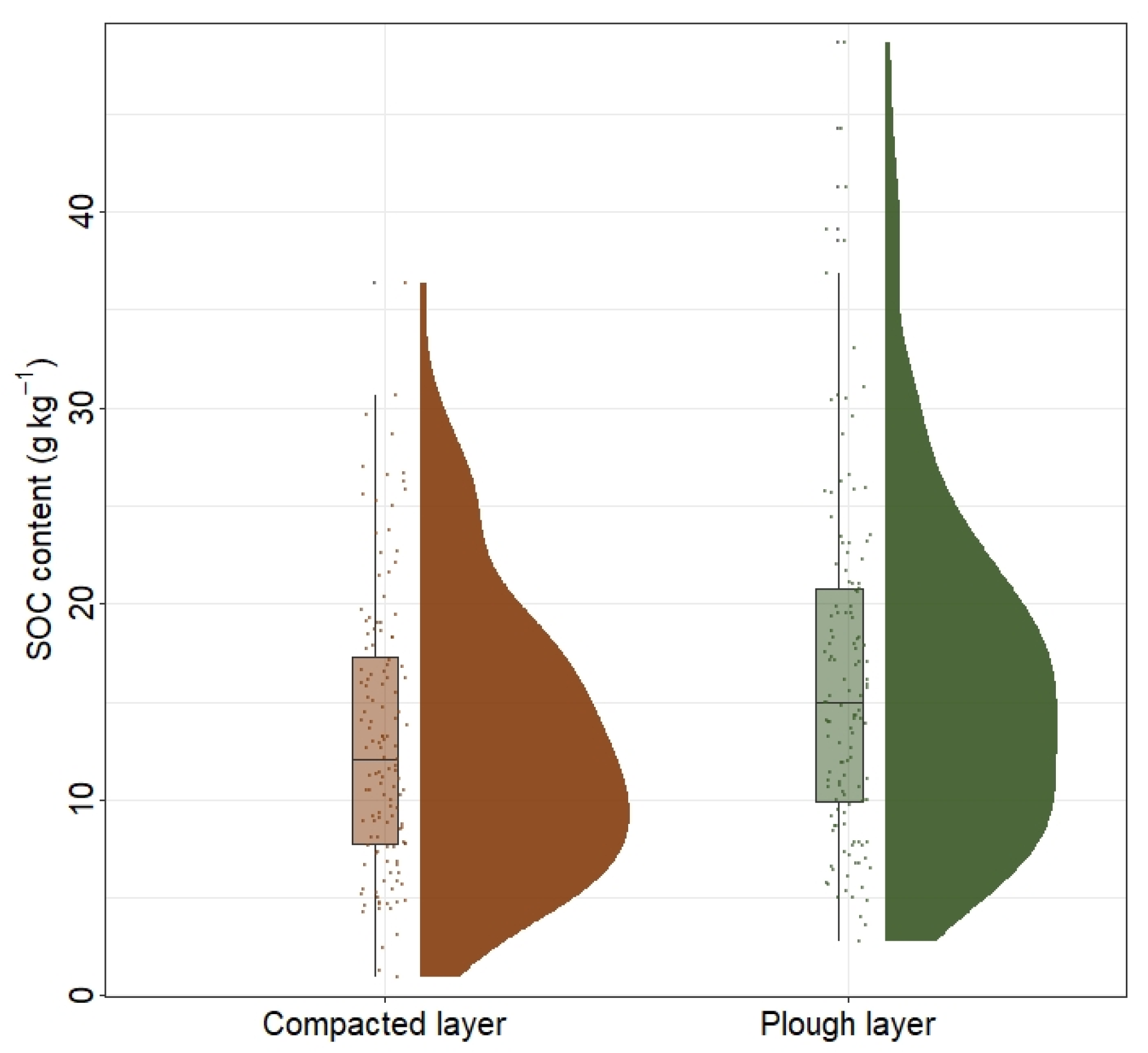
The plough and compacted layer depths of 132 sampling points are shown in Table 2 and Figure S3. The average depths of the plough layer and compacted layer were 16.29 cm (5.00–27.50 cm) and 7.39 cm (2.50–20.00 cm), respectively. The third quantiles of the two layers were 20.00 and 10.00 cm, indicating the depths of almost all sampling sites belonged to the intervals. Hence, we determined the plough layer as the 0–20 cm depth and the compacted layer as the 20–30 cm depth, respectively. In the plough layer, SOC varied from 2.78 to 48.65 g kg−1, with the average and median SOC at 16.33 and 14.93 g kg−1, respectively. In the compacted layer, SOC varied from 0.96 to 36.40 g kg−1, with the average and median SOC at 13.21 and 12.09 g kg−1, respectively (Figure 2 and Table 2). The skewness values were 1.12 and 0.72 in two layers, indicating a slightly positive skewness distribution. The kurtosis of 4.56 and 3.19 showed that the data was lightly tailed. There were high variations in two layers, with the %CV of 53.88 and 52.91 % and the SD of 8.80 and 6.99 g kg−1 [61]. As a result of the Kolmogorov–Smirnov tests, SOC in two layers slightly deviated from normality [62].

3.2. Model Accuracy and Uncertainty

The average of three indices (i.e., R2, RMSE, and U) through 50 repetitions showed model performance, i.e., accuracy and uncertainty (Table 3). Compared with the compacted layer, the accuracy in the plough layer was slightly higher both in CV (R2: 0.68 and 0.58 in the plough and compacted layer) and OOB (R2: 0.61 and 0.54). The U (1.09 and 1.05) showed that the uncertainty was also relatively lower in the plough layer. Moreover, the PICP (0.88 and 0.86) confirmed that the 90% CI derived by QRF was efficacious.
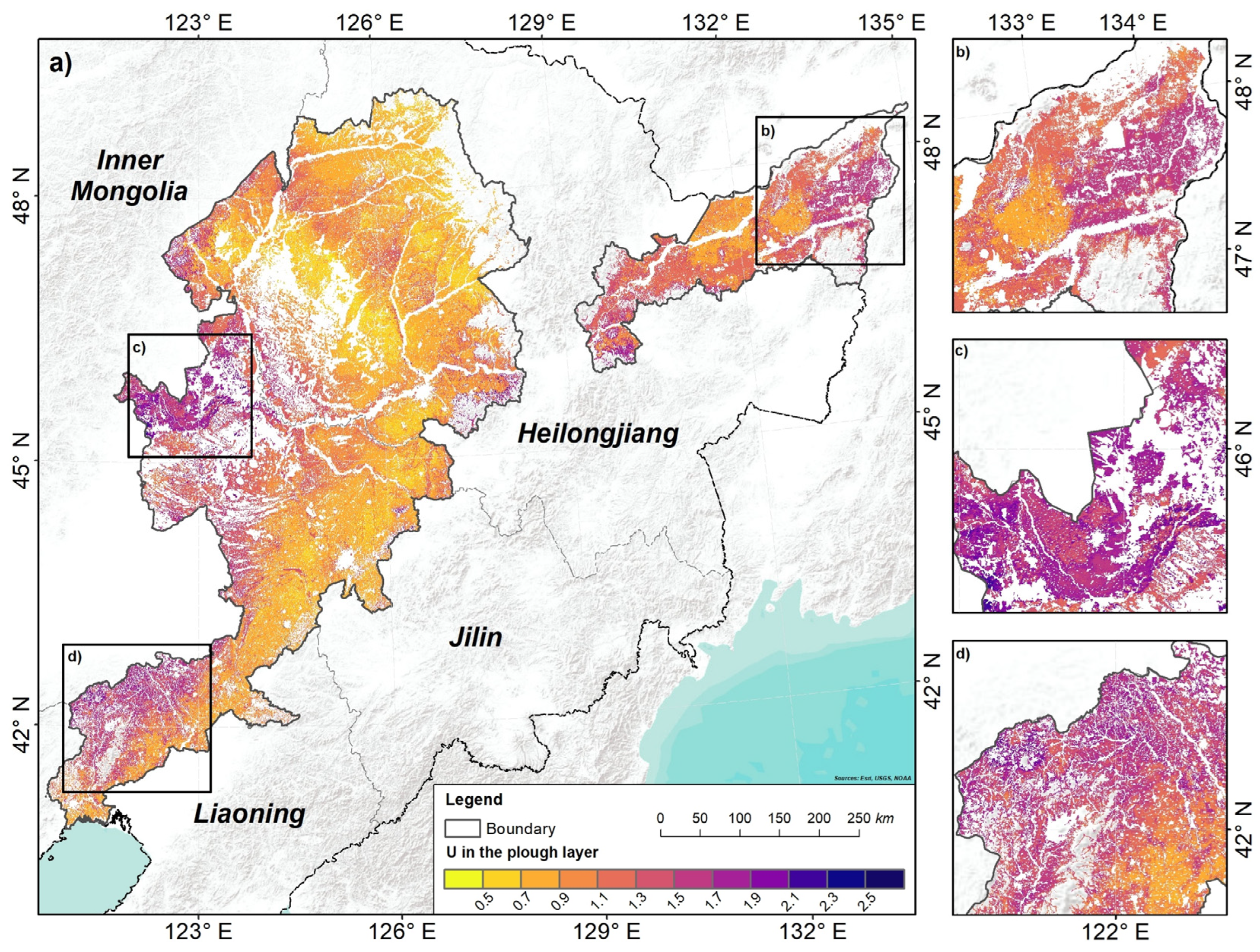
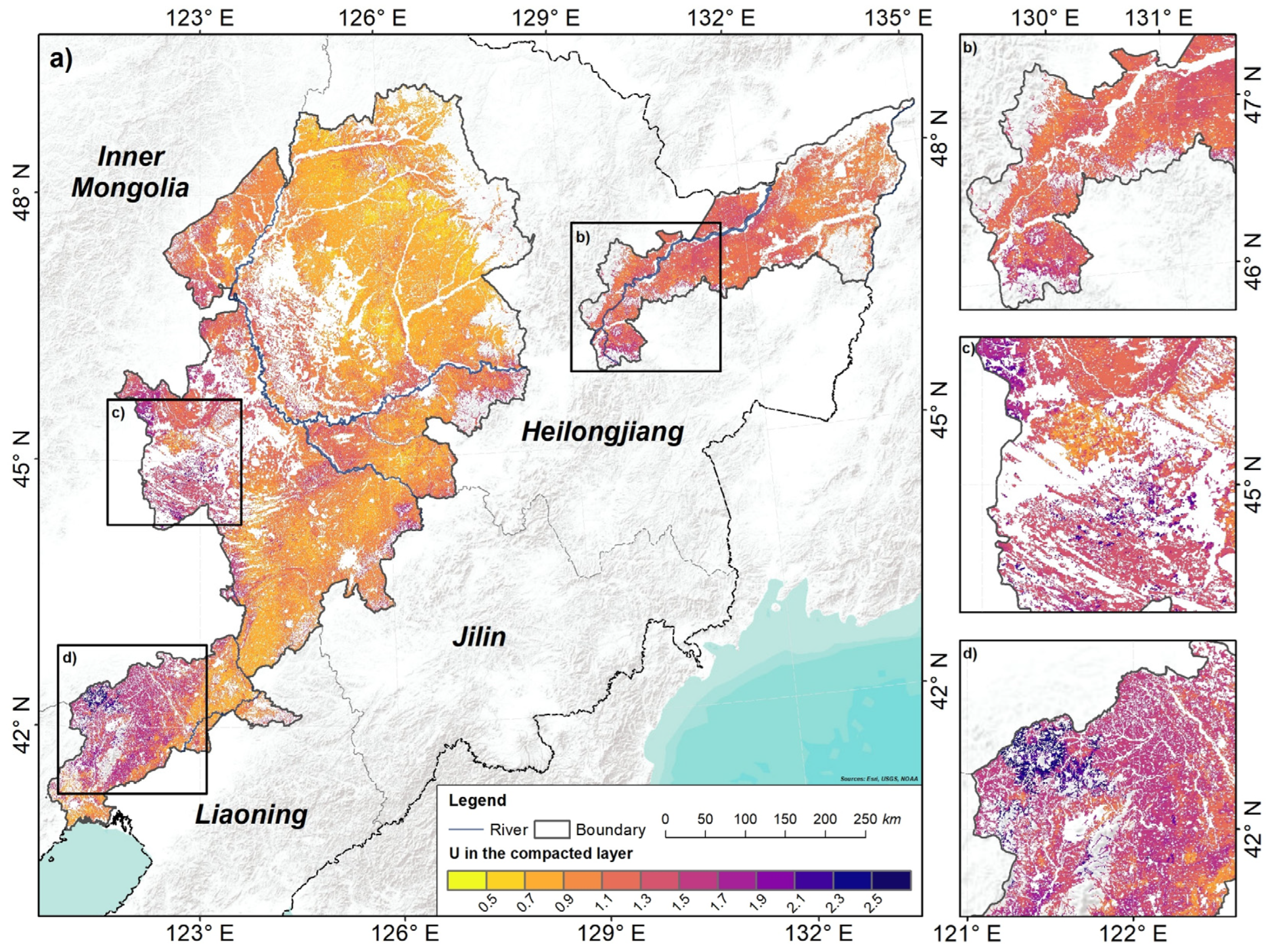
The spatial distribution pattern of uncertainty was shown in Figure 3a and Figure 4a. There was a great similarity in the spatial distribution of prediction uncertainty at two layers with averages of 1.04 (plough layer) and 1.07 (compacted layer). We found there was lower uncertainty in the middle of Songnen Plain with large areas of croplands. Meanwhile, the relatively higher uncertainty occurred in the western and southwestern areas of Songnen Plain, the north and south sides of Sanjiang Plain, and the west side of Liaohe Plain, where there were relatively scattered fields and varied land-use types (Figure 3 and Figure 4).

3.3. Importance of Environmental Covariates

Feature selection and modeling evaluation were used to estimate the importance of environmental covariates. Firstly, Boruta was used to reduce environmental covariates from 141 to 40 (soil and parent material: 16–7, climate: 32–15, organism: 54–8, relief: 29–4, position: 10–6).
In Boruta, the Z score varied from 3.19 to 11.91 on average. The variable interpretability based on the average Z score can be divided into three levels, i.e., low (<5), medium (5–10), and high relevance (>10). There were four soil and parent material variables (Silt, Sand, BSI, GI), four climate variables (BIO03, BIO07, BIO13, Tmax), three organism variables (CroCANIa: the average of CANI during the growth period of crops, NCroFPARa and NCroLAIa: the average of FPAR and LAI during the non-growth period of crops), three relief variables (ELE, VD, TWI), and one position variable (OGC60: OGC at 60°) in the low relevance level. A total of 20 variables in the medium relevance level, including three soil and parent material variables (SE, BI, CarI), nine climate variables (BIO04, BIO08, BIO09, BIO10, LSTD, LSTN, Sol, Tmin, VP), five organism variables (NCroNDRIa, NCroGPPa and NCroNPPa: the average of NDRI, GPP and NPP during the non-growth period of crops, NCroGPPv, and NCroNPPv: the variance of GPP and NPP during the non-growth period of crops), 1 relief variable (CNBL), and two position variables (OGC30 and OGC120: OGC at 30° and 120°. The left two climate variables (BIO11, Tavg) and three position variables (OGC45, OGC105 and OGC165: OGC at 45°, 105°, and 165°) were in the high relevance level.
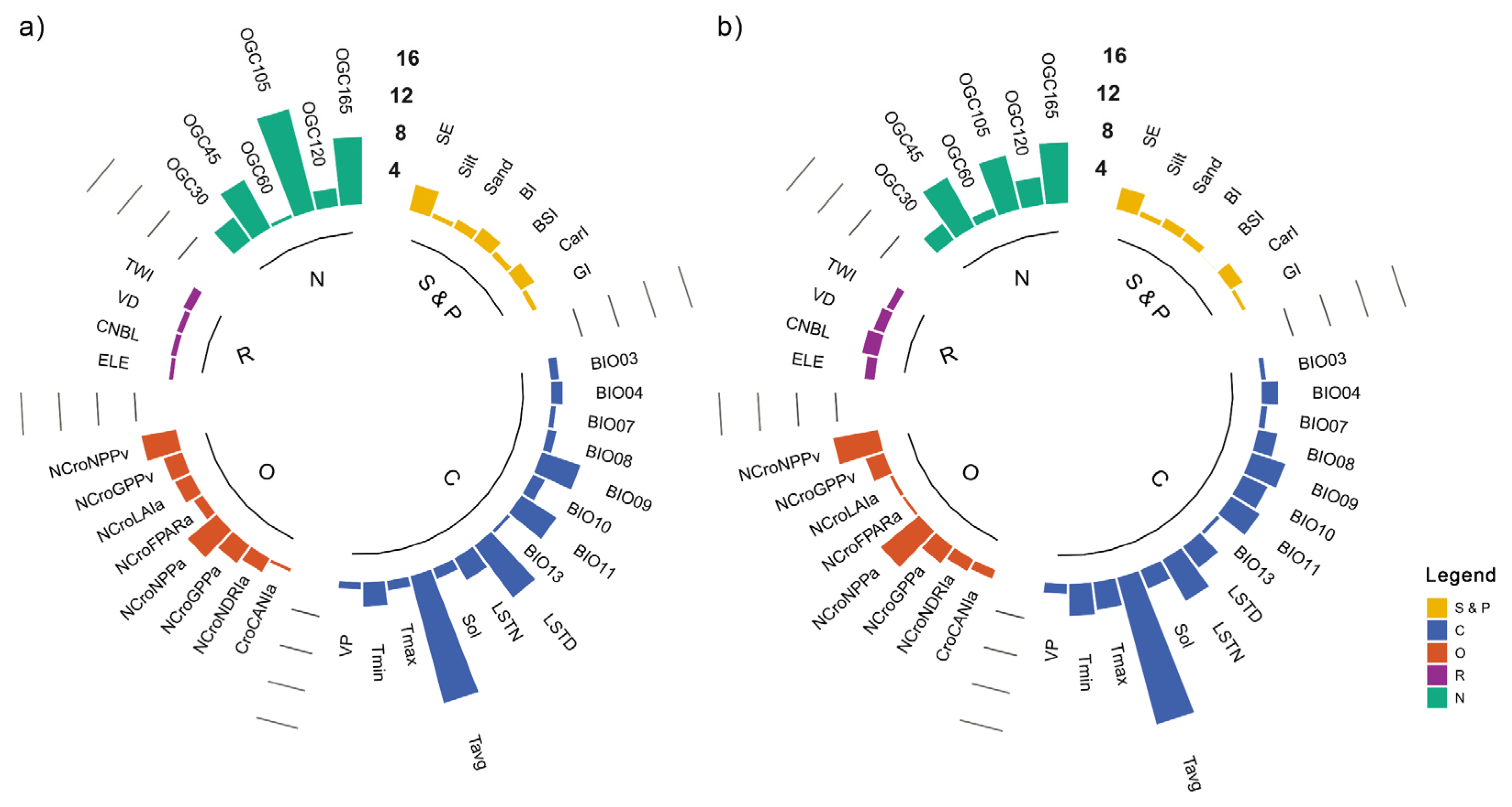
Secondly, the %IncMSE of variables in the QRF model was used to subsequently explain the contributions of environmental covariates (Figure 5 and Figure 6). There were significant differences of relative importance in five environmental covariates. Climate was the main controlling factor, with a relative importance of 42.56% and 48.02% in two layers, followed by position (29.27% and 23.91%), organism (16.88% and 16.88%), soil and parent material (8.74% and 6.56%), and relief (2.55% and 4.63%). Compared with the plough layer, the relative importance of the climate and relief was higher in the compacted layer, which was derived from the reduction in soil and parent material and the position. The change of relative importance in detailed variables is shown in Figure 6. To be more specific, Tavg (plough layer: 13.84%, compacted layer: 15.87%), LSTD (6.82%, 2.73%), LSTN (2.62%, 4.92%), and BIO09 (4.29%, 3.62%) were the dominant sub-climate variables. The NCroNPPa (3.95%, 5.16%) and NCroNPPv (3.71%, 4.69%) could explain most of the organism information, especially in the compacted layer. The position contributed more to the model in the plough layers, especially in OGC105 (11.05%, 5.80%), OGC165 (7.11%, 6.36%), and OGC45 (5.79%, 5.88%).

3.4. Spatial Distribution Pattern of SOC

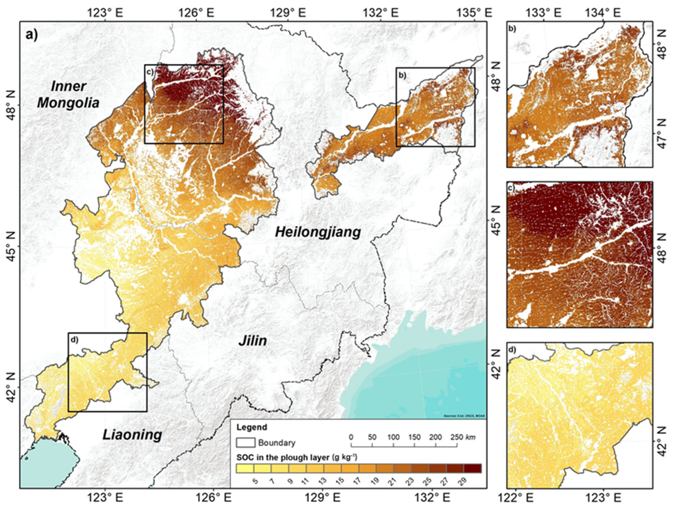
The spatial predictions of SOC at two layers are shown in Figure 7a and Figure 8a. The cropland SOC overall increased from the southern to northern areas, whereas there were some differences in the three sub-plains. The average SOC was 17.34 g kg−1 (4.99–37.65) in the plough layer. In the Songnen Plain, higher SOC occurred in the northern area with higher altitudes (Figure 7c). In Liaohe Plain, the SOC with an average of 9.18 g kg−1 was relatively lower and evenly distributed. Compared with another two plains, the highest SOC was in the Sanjiang Plain, with an average of 21.78 g kg−1 (16.68–34.33). Notably, we found that the area with high SOC was widely distributed in the cropland close to forestlands, i.e., southeastern and northwestern (Figure 7b).
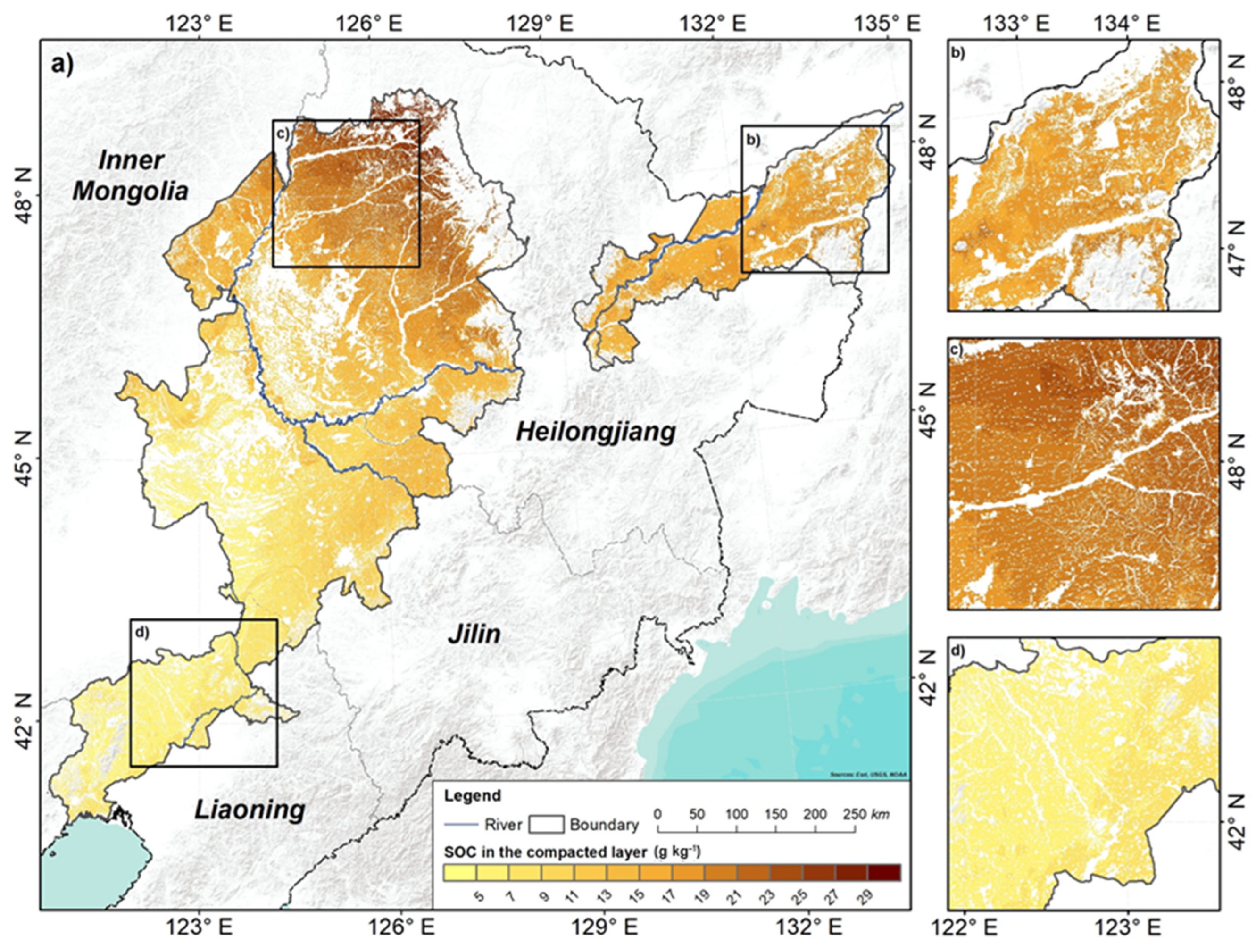
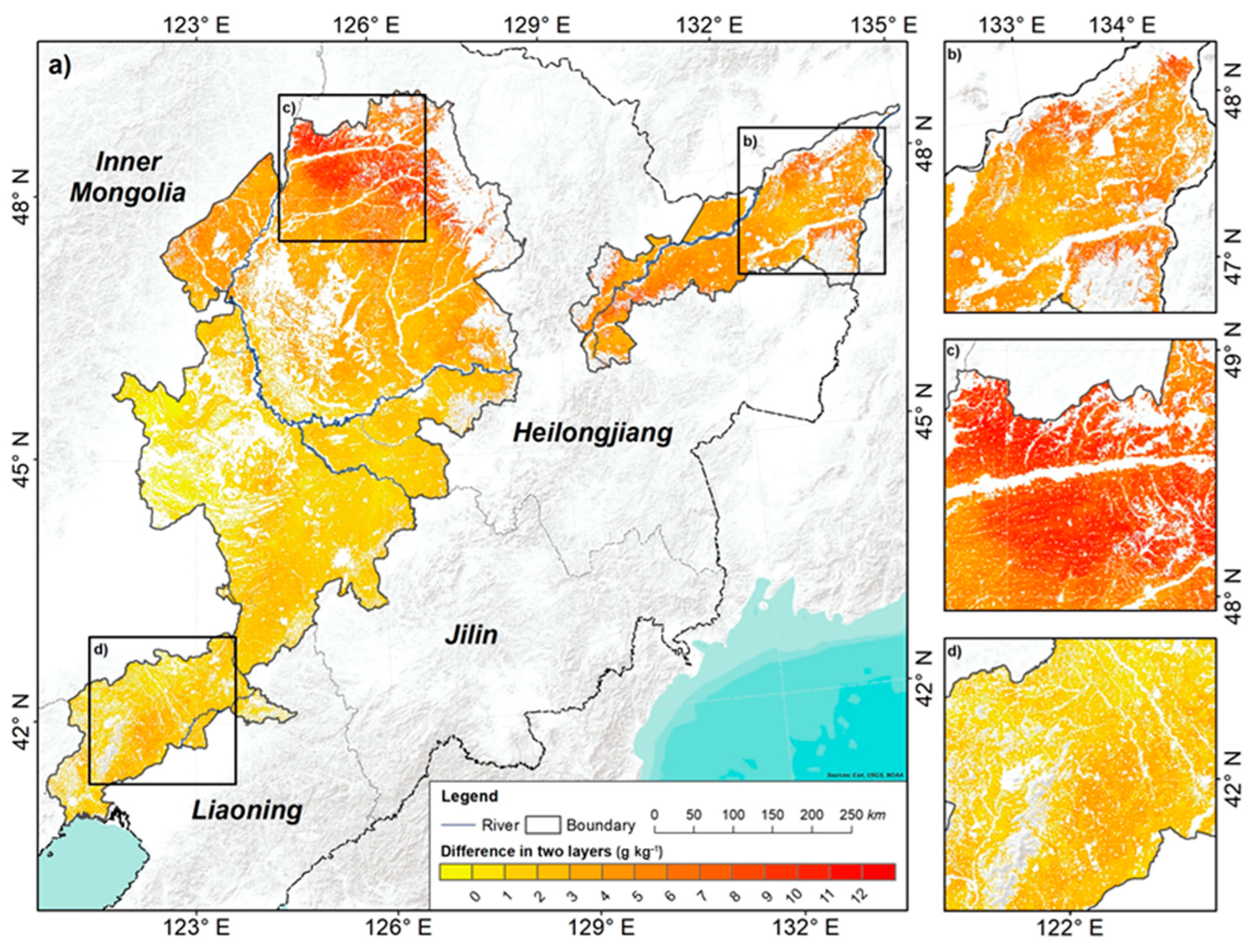
The spatial distribution of compacted layers was similar to that in plough layers, whereas the content was generally lower (Northeast Plain: 13.92, Liaohe Plain: 7.01, Songnen Plain: 14.85, Sanjiang Plain: 16.70 g kg−1) (Figure 8). We subsequently analysed the vertical differences of SOC in two layers (Figure 9). SOC decreased by an average of 3.41 g kg−1 and northern areas decreased more than southern areas. Notably, we found that there was usually a great decrease in the area with high SOC (e.g., medium area of Liaohe Plain, northern area of Songnen Plain, and northeastern area of Sanjiang Plain) (Figure 8b–d). In contrast, there was less change in intensive cropland areas, especially in the southwestern Songnen Plain, where the change of SOC was almost equal to zero.

4. Discussion

4.1. Feature Selection

We performed QRF models using full and Boruta selected covariates. The results showed that 70% of covariates were filtered by the Boruta algorithm, whereas the accuracy was almost similar (CV R2, 0–20 cm: 0.67 for the initial database and 0.68 for the selected database, 20–30 cm: 0.58 and 0.58) and the uncertainty saw a downward trend (U, 0–20 cm: 1.05 and 1.15, 20–30 cm: 1.09 and 1.20 for the selected and the initial database) after feature selection. Our results showed that eliminating the redundant variables before modeling can actually improve model parsimony and accuracy [63].
We found a noticeable decrease in vegetation indices and productivity products during the growth period of crops. We suppose frequent human distribution (e.g., irrigation and fertilization) weakens the correlation between vegetation and SOC, while vegetation during the non-growth period of crops can better reflect the carrying capacity of cropland soil in natural conditions. Meanwhile, since relief covariates were derived from DEM, there was high multicollinearity, leading to a decrease after Boruta. By contrast, many climate covariates remained, which indicated that climate might play a crucial role in the predictions of SOC at a regional scale.

4.2. Model Accuracy

The average R2 (CV) in our study was 0.68 and 0.58 at two depths, which exceeded the average R2 (0.49) in broad-scale SOC DSM studies, indicating QRF had better performance in the area [7]. Notably, we found more deviation in low and high SOC (Figure S1). That is because bagging ensemble algorithms aggravate the final prediction from multiple individual predictors, which can improve robustness but reduce sensitivity to extremums [49]. Compared with the plough layer, the model accuracy in the compacted layer was lower. That is because there is a higher coefficient of variation and SD in the compacted layer (Table 2), which may have negative effects on model fitness [64]. Additionally, environmental covariates were almost driven from satellites and meteorological stations, which can reflect more land surface information.

4.3. Uncertainty Assessments

The spatial distribution pattern of U is shown in Figure 3, Figure 4 and Figure S2. On the one hand, the uncertainty is from the heterogeneity of the spatial characteristics. We found relatively high uncertainty in the southwestern area of Songnen Plain, the western Liaohe Plain, and northern and southern Sanjiang Plain, with fragmented fields, various land-use types, or dramatically changeable altitudes. As environmental characteristics greatly change in these areas, the correlations between SOC and covariates are complicated and unquantifiable, which leads to the lack of information on model fitness and a decrease in model stability [17]. On the other hand, the deviation in multi-source data products and in the resampling procedure may be propagated into the predictions [65].
Additionally, predictions in the compacted layer were slightly higher than in the plough layer. That is because almost all covariates from satellites can only directly reflect topsoil information, while the downward trend of the correlations with depths getting deeper is nonlinear, which has negative effects on the accuracy and uncertainty of predictions.

4.4. Spatial Distribution Pattern of SOC and Controlling Factors

The spatial distribution pattern could be explained by environmental covariates [1]. Figure 5 and Figure 6 showed climate was the dominant control factor, which was consistent with previous studies in broad region scales [66,67]. That is because in broad region scales, attainable SOC is the vital factor to cause differences in SOC distribution, and climate determines the process and intensity of the weathering of parent materials and carbon input by vegetation [68,69]. In our study, several variables on behalf of temperature play a crucial role in climate, i.e., Tavg, LSTD, BIO09, and LSTN, which are more important than covariates related to precipitation in the study area. That may be because in croplands, the effect of precipitation can be partly offset by irrigation regulation, thus temperature which affects the microbial decomposition process is more representative of the impact of nature’s climate on soil [1]. The position on behalf of the spatial information in data was the second important environmental covariate. This indicates a spatial trend of SOC in the area, especially at 105°, which is generally consistent with the direction of the monsoon in the area [34]. We found NCroNPPa and NCroNPPv contributed the most in organism covariates. That is because NPP is the direct factor of vegetation productivity and determines the amounts of plant litter, which influences the input and decomposition processes of SOC [1]. Additionally, the lower variability of elevation (100–200 m) and soil types limits the contribution of relief, soil, and parent material to the models.
For vertical scales, due to the relatively incomplete mineralization, SOC was overall lower in the compacted layers. Notably, we found the downward trend was relatively flat in the intensive cropland area (e.g., the middle of Songnen Plain). That may be because there is large-scale mechanized operation and a relatively long-term cultivation history in flat terrain, causing a strong disturbance in the two layers and a decrease in differences [5].

4.5. Perspectives and Limitation

This study illustrated the spatial distribution pattern of cropland SOC in the Northeast China Plain using the DSM method and optimal environmental covariates. There are several limitations, as follows.
Firstly, more advanced feature selection methods should be considered to improve model performance. Though Boruta could greatly decrease the number of environment covariates, there was less improvement in accuracy and uncertainty. Numerous DSM studies performed feature selection (e.g., Forward Recursive Feature Selection, Recursive Feature Elimination) before fitting the models, whereas few studies are focusing on providing the validity domain on the applicability of different feature selection algorithms in different situations [17,70,71,72,73]. Further studies should solve the knowledge gap and find an algorithm that can select the most important covariates directly related to the target model and improve model performance.
Moreover, it is essential to map SOC for the areas with less differences and with more sampling points. We found irregular SOC changes in some areas at the vertical scale (e.g., the middle of Songnen Plain). Further studies should focus on fitting models with more sampling points and try to fit the model with train, validation, and test datasets, which could generate more accurate SOC maps and help illustrate the impacts of long-term mechanized operation.
Finally, more environmental covariates with higher spatio-temporal resolutions need to be proposed and used to model. Although climate has a lagged effect on the spatial distribution of SOC and WorldClim2 from 1970 to 2000 at 1 km spatial resolution has been widely used in DSM, there is a lack of WorldClim2 products for the last 20 years. Feature studies should apply spatio-temporal downscaling methods to produce new climate products to minimize the error and uncertainty in predictions due to covariates.

5. Conclusions

This study revealed the up-to-date regional spatial distribution pattern of cropland SOC in the plough layer and compacted layer of the Northeast China Plain, which could provide a reference for evaluating SOC spatial distribution patterns after long-term cultivation. The major conclusions were as follows:
(1)
Boruta was a compelling feature selection method to eliminate redundant variables and develop the optimal QRF model.
(2)
SOC overall increased from the southern to the northern areas, with an average of 17.34 g kg−1 in the plough layer and 13.92 g kg−1 in the compacted layer. At the vertical scale, SOC decreased, with depths getting deeper. The average decreasing SOC is 3.41 g kg−1, and the northern area decreased more than the southern area.
(3)
Climate (i.e., average temperature, daytime and nighttime land surface temperature, and mean temperature of driest quarter) was the dominant controlling factor, followed by position (i.e., oblique geographic coordinate at 105°), and organism (i.e., the average and variance of net primary productivity in the non-crop period).
(4)
The average uncertainty values were 1.04 in the plough layer and 1.07 in the compacted layer. The high uncertainty appeared in the areas with relatively scattered fields, high altitudes, and complex landforms.

Supplementary Materials

The following supporting information can be downloaded at: https://www.mdpi.com/article/10.3390/rs15205033/s1, Figure S1: Scatter plot of SOC predictions (CV dataset) and SOC observations in (a) the plough layer and (b) the compacted layer; Figure S2. Spatial distribution pattern of 5% quantile predictions (a and e), average predictions (b and f), 95% quantile predictions (c and g) and uncertainty (d and h) in the plough layer and the compacted layer; Figure S3. Spatial distribution of the thickness of (a) the plough layer and (b) the compacted layer; Table S1: List of environmental covariates in the database.

Author Contributions

Conceptualization, X.Z. and Z.Z.; methodology, X.Z. and Z.S.; software, X.Z. and J.X.; validation, Z.Z., N.W. and T.X.; formal analysis, X.C.; investigation, Y.X.; resources, Y.H.; data curation, Z.Z.; writing—original draft preparation, X.Z.; writing—review and editing, J.X. and S.C.; visualization, T.X.; supervision, Z.S.; project administration, S.C.; funding acquisition, Z.S. All authors have read and agreed to the published version of the manuscript.

Funding

This study was supported by the National Natural Science Foundation of China (U1901601), the National Key Research and Development Program of China (2022YFB3903503).

Institutional Review Board Statement

Not applicable.

Informed Consent Statement

Not applicable.

Data Availability Statement

The code is available upon reasonable request to the corresponding author.

Conflicts of Interest

The authors declare no conflict of interest.

References

  1. Wiesmeier, M.; Urbanski, L.; Hobley, E.; Lang, B.; von Lutzow, M.; Marin-Spiotta, E.; van Wesemael, B.; Rabot, E.; Liess, M.; Garcia-Franco, N.; et al. Soil organic carbon storage as a key function of soils-A review of drivers and indicators at various scales. Geoderma 2019, 333, 149–162. [Google Scholar] [CrossRef]
  2. Zomer, R.J.; Bossio, D.A.; Sommer, R.; Verchot, L.V. Global Sequestration Potential of Increased Organic Carbon in Cropland Soils. Sci. Rep. 2017, 7, 15554. [Google Scholar] [CrossRef] [PubMed]
  3. Robinson, D.A.; Emmett, B.A.; Reynolds, B.; Rowe, E.C.; Spurgeon, D.; Keith, A.M.; Lebron, I.; Hockley, N.; Hester, R.; Harrison, R. Soil natural capital and ecosystem service delivery in a world of global soil change. Soils Food Secur. 2012, 35, 41. [Google Scholar]
  4. Xue, J.; Zhang, X.L.; Chen, S.C.; Hu, B.F.; Wang, N.; Shi, Z. Quantifying the agreement and accuracy characteristics of four satellite-based LULC products for cropland classification in China. J. Integr. Agric. 2023. [Google Scholar] [CrossRef]
  5. Zhuo, Z.Q.; Xing, A.; Cao, M.; Li, Y.; Zhao, Y.Z.; Guo, X.L.; Huang, Y.F. Identifying the position of the compacted layer by measuring soil penetration resistance in a dryland farming region in Northeast China. Soil Use Manag. 2020, 36, 494–506. [Google Scholar] [CrossRef]
  6. Colombi, T.; Braun, S.; Keller, T.; Walter, A. Artificial macropores attract crop roots and enhance plant productivity on compacted soils. Sci. Total Environ. 2017, 574, 1283–1293. [Google Scholar] [CrossRef]
  7. Chen, S.; Arrouays, D.; Mulder, V.L.; Poggio, L.; Minasny, B.; Roudier, P.; Libohova, Z.; Lagacherie, P.; Shi, Z.; Hannam, J.J.G. Digital mapping of GlobalSoilMap soil properties at a broad scale: A review. Geoderma 2022, 409, 115567. [Google Scholar] [CrossRef]
  8. Arrouays, D.; Poggio, L.; Guerrero, O.A.S.; Mulder, V.L. Digital soil mapping and GlobalSoilMap. Main advances and ways forward. Geoderma Reg. 2020, 21, e00265. [Google Scholar] [CrossRef]
  9. Tziolas, N.; Tsakiridis, N.; Chabrillat, S.; Demattê, J.A.; Ben-Dor, E.; Gholizadeh, A.; Zalidis, G.; Van Wesemael, B. Earth observation data-driven cropland soil monitoring: A review. Remote Sens. 2021, 13, 4439. [Google Scholar] [CrossRef]
  10. Poggio, L.; de Sousa, L.M.; Batjes, N.H.; Heuvelink, G.B.M.; Kempen, B.; Ribeiro, E.; Rossiter, D. SoilGrids 2.0: Producing soil information for the globe with quantified spatial uncertainty. Soil 2021, 7, 217–240. [Google Scholar] [CrossRef]
  11. Safanelli, J.L.; Dematte, J.A.M.; Chabrillat, S.; Poppiel, R.R.; Rizzo, R.; Dotto, A.C.; Silvero, N.E.Q.; Mendes, W.D.; Bonfatti, B.R.; Ruiz, L.F.C.; et al. Leveraging the application of Earth observation data for mapping cropland soils in Brazil. Geoderma 2021, 396, 115042. [Google Scholar] [CrossRef]
  12. Liang, Z.; Chen, S.; Yang, Y.; Zhao, R.; Shi, Z.; Viscarra Rossel, R.A. National digital soil map of organic matter in topsoil and its associated uncertainty in 1980’s China. Geoderma 2019, 335, 47–56. [Google Scholar] [CrossRef]
  13. Chen, S.; Liang, Z.; Webster, R.; Zhang, G.; Zhou, Y.; Teng, H.; Hu, B.; Arrouays, D.; Shi, Z. A high-resolution map of soil pH in China made by hybrid modelling of sparse soil data and environmental covariates and its implications for pollution. Sci. Total Environ. 2019, 655, 273–283. [Google Scholar] [CrossRef] [PubMed]
  14. Zhou, Y.; Xue, J.; Chen, S.C.; Zhou, Y.; Liang, Z.Z.; Wang, N.; Shi, Z. Fine-Resolution Mapping of Soil Total Nitrogen across China Based on Weighted Model Averaging. Remote Sens. 2020, 12, 85. [Google Scholar] [CrossRef]
  15. Keskin, H.; Grunwald, S.; Harris, W.G. Digital mapping of soil carbon fractions with machine learning. Geoderma 2019, 339, 40–58. [Google Scholar] [CrossRef]
  16. Ye, Y.; Fang, X.Q.; Ren, Y.Y.; Zhang, X.Z.; Chen, L. Cropland cover change in Northeast China during the past 300 years. Sci. China Ser. D 2009, 52, 1172–1182. [Google Scholar] [CrossRef]
  17. Zhang, X.L.; Xue, J.; Chen, S.C.; Wang, N.; Shi, Z.; Huang, Y.F.; Zhuo, Z.Q. Digital Mapping of Soil Organic Carbon with Machine Learning in Dryland of Northeast and North Plain China. Remote Sens. 2022, 14, 2504. [Google Scholar] [CrossRef]
  18. Wang, S.; Zhou, M.Y.; Adhikari, K.; Zhuang, Q.L.; Bian, Z.X.; Wang, Y.; Jin, X.X. Anthropogenic controls over soil organic carbon distribution from the cultivated lands in Northeast China. Catena 2022, 210, 105897. [Google Scholar] [CrossRef]
  19. Zhou, Y.; Hartemink, A.E.; Shi, Z.; Liang, Z.; Lu, Y. Land use and climate change effects on soil organic carbon in North and Northeast China. Sci. Total Environ. 2019, 647, 1230–1238. [Google Scholar] [CrossRef]
  20. Guo, L.; Sun, X.R.; Fu, P.; Shi, T.Z.; Dang, L.N.; Chen, Y.Y.; Linderman, M.; Zhang, G.L.; Zhang, Y.; Jiang, Q.H.; et al. Mapping soil organic carbon stock by hyperspectral and time-series multispectral remote sensing images in low-relief agricultural areas. Geoderma 2021, 398, 115118. [Google Scholar] [CrossRef]
  21. Nachtergaele, F.; Velthuizen, H.; Verelst, L.; Wiberg, D.J.F. Food and Agriculture Organization of the United Nations, Rome Harmonized World Soil Database (HWSD); Food and Agriculture Organization of the United Nations: Rome, Italy, 2009. [Google Scholar]
  22. Kendall, M.G. Rank Correlation Methods; American Psychological Association: Worcester, MA, USA, 1948. [Google Scholar]
  23. Bao, S. Soil Agro-Chemistrical Analysis; China Agriculture Press: Beijing, China, 2000; Volume 2030, pp. 30–107. [Google Scholar]
  24. McBratney, A.B.; Santos, M.L.M.; Minasny, B. On digital soil mapping. Geoderma 2003, 117, 3–52. [Google Scholar] [CrossRef]
  25. Irons, J.R.; Dwyer, J.L.; Barsi, J.A. The next Landsat satellite: The Landsat Data Continuity Mission. Remote Sens. Environ. 2012, 122, 11–21. [Google Scholar] [CrossRef]
  26. Foga, S.; Scaramuzza, P.L.; Guo, S.; Zhu, Z.; Dilley, R.D.; Beckmann, T.; Schmidt, G.L.; Dwyer, J.L.; Hughes, M.J.; Laue, B. Cloud detection algorithm comparison and validation for operational Landsat data products. Remote Sens. Environ. 2017, 194, 379–390. [Google Scholar] [CrossRef]
  27. Teng, H.F.; Hu, J.; Zhou, Y.; Zhou, L.Q.; Shi, Z. Modelling and mapping soil erosion potential in China. J. Integr. Agr. 2019, 18, 251–264. [Google Scholar] [CrossRef]
  28. Hengl, T.; Mendes de Jesus, J.; Heuvelink, G.B.; Ruiperez Gonzalez, M.; Kilibarda, M.; Blagotic, A.; Shangguan, W.; Wright, M.N.; Geng, X.; Bauer-Marschallinger, B.; et al. SoilGrids250m: Global gridded soil information based on machine learning. PLoS ONE 2017, 12, e0169748. [Google Scholar] [CrossRef]
  29. Fick, S.E.; Hijmans, R.J. WorldClim 2: New 1-km spatial resolution climate surfaces for global land areas. Int. J. Climatol. 2017, 37, 4302–4315. [Google Scholar] [CrossRef]
  30. Wan, Z.; Hook, S.; Hulley, G. MOD11A1 MODIS/Terra Land Surface Temperature/Emissivity Daily L3 Global 1km SIN Grid V006 [Data set]. NASA EOSDIS Land Processes DAAC. 2015. Available online: https://lpdaac.usgs.gov/products/mod11a1v006/ (accessed on 26 November 2022).
  31. Myneni, R.; Knyazikhin, Y.; Park, T. MODIS/Terra+Aqua Leaf Area Index/FPAR 4-Day L4 Global 500m SIN Grid V061 [Data Set]; Land Processes Distributed Active Archive Center: Sioux Falls, SD, USA, 2021. [CrossRef]
  32. Running, S.; Mu, Q.; Zhao, M. MOD17A2H MODIS/Terra Gross Primary Productivity 8-Day L4 Global 500m SIN Grid V006 [Data Set]; Land Processes Distributed Active Archive Center: Sioux Falls, SD, USA, 2015. [CrossRef]
  33. Jarvis, A.; Reuter, H.I.; Nelson, A.; Guevara, E. Hole-filled SRTM for the globe Version 4, available from the CGIAR-CSI SRTM 90m Database. 2008. Available online: https://srtm.csi.cgiar.org (accessed on 9 November 2018).
  34. Møller, A.B.; Beucher, A.M.; Pouladi, N.; Greve, M.H. Oblique geographic coordinates as covariates for digital soil mapping. Soil 2020, 6, 269–289. [Google Scholar] [CrossRef]
  35. Schad, P.; Dondeyne, S.; Lal, R. World Reference Base for Soil Resources 2014, Update 2015: International Soil Classification System for Naming Soils and Creating Legends for Soil Maps; Fao: Rome, Italy, 2015. [Google Scholar]
  36. Hartmann, J.; Moosdorf, N. The new global lithological map database GLiM: A representation of rock properties at the Earth surface. Geochem. Geophys. Geosystems 2012, 13. [Google Scholar] [CrossRef]
  37. Zhuo, Z.Q.; Chen, Q.Q.; Zhang, X.L.; Chen, S.C.; Gou, Y.X.; Sun, Z.X.; Huang, Y.F.; Shi, Z. Soil organic carbon storage, distribution, and influencing factors at different depths in the dryland farming regions of Northeast and North China. Catena 2022, 210, 105934. [Google Scholar] [CrossRef]
  38. Running, S.; Mu, Q.; Zhao, M. MOD16A2 MODIS/Terra Net Evapotranspiration 8-Day L4 Global 500m SIN Grid V006 [Data set], NASA EOSDIS Land Processes DAAC. 2017. Available online: https://lpdaac.usgs.gov/products/mod16a2v006/ (accessed on 9 January 2020).
  39. Mladenova, I.E.; Bolten, J.D.; Crow, W.T.; Sazib, N.; Cosh, M.H.; Tucker, C.J.; Reynolds, C. Evaluating the Operational Application of SMAP for Global Agricultural Drought Monitoring. IEEE J. Sel. Top. Appl. Earth Obs. Remote Sens. 2019, 12, 3387–3397. [Google Scholar] [CrossRef]
  40. Riggs, G.A.; Hall, D.K.; Salomonson, V.V. A snow index for the Landsat thematic mapper and moderate resolution imaging spectroradiometer. In Proceedings of the IGARSS’94-1994 IEEE International Geoscience and Remote Sensing Symposium, Pasadena, CA, USA, 8–12 August 1994; pp. 1942–1944. [Google Scholar]
  41. Zhang, M.; Wu, B.F.; Zeng, H.W.; He, G.J.; Liu, C.; Tao, S.Q.; Zhang, Q.; Nabil, M.; Tian, F.Y.; Bofana, J.; et al. GCI30: A global dataset of 30 m cropping intensity using multisource remote sensing imagery. Earth Syst. Sci. Data 2021, 13, 4799–4817. [Google Scholar] [CrossRef]
  42. You, N.; Dong, J.; Huang, J.; Du, G.; Zhang, G.; He, Y.; Yang, T.; Di, Y.; Xiao, X. The 10-m crop type maps in Northeast China during 2017-2019. Sci. Data 2021, 8, 41. [Google Scholar] [CrossRef]
  43. Conrad, O.; Bechtel, B.; Bock, M.; Dietrich, H.; Fischer, E.; Gerlitz, L.; Wichmann, V.; Böhner, J. System for automated geoscientific analyses (SAGA) v. 2.1. 4. Geoscientific Model Development 2015, 8(7), 1991–2007. [Google Scholar] [CrossRef]
  44. Gorelick, N.; Hancher, M.; Dixon, M.; Ilyushchenko, S.; Thau, D.; Moore, R. Google Earth Engine: Planetary-scale geospatial analysis for everyone. Remote Sens. Environ. 2017, 202, 18–27. [Google Scholar] [CrossRef]
  45. Kursa, M.B.; Rudnicki, W.R. Feature selection with the Boruta package. J. Stat. Softw. 2010, 36, 1–13. [Google Scholar] [CrossRef]
  46. Stoppiglia, H.; Dreyfus, G.; Dubois, R.; Oussar, Y.J. Ranking a random feature for variable and feature selection. J. Mach. Learn. Res. 2003, 3, 1399–1414. [Google Scholar]
  47. Amiri, M.; Pourghasemi, H.R.; Ghanbarian, G.A.; Afzali, S.F. Assessment of the importance of gully erosion effective factors using Boruta algorithm and its spatial modeling and mapping using three machine learning algorithms. Geoderma 2019, 340, 55–69. [Google Scholar] [CrossRef]
  48. Meinshausen, N.; Ridgeway, G. Quantile regression forests. J. Mach. Learn. Res. 2006, 7, 983–999. [Google Scholar]
  49. Breiman, L. Random forests. Mach. Learn. 2001, 45, 5–32. [Google Scholar] [CrossRef]
  50. Lalitha, M.; Dharumarajan, S.; Suputhra, A.; Kalaiselvi, B.; Hegde, R.; Reddy, R.S.; Shiva Prasad, C.R.; Harindranath, C.S.; Dwivedi, B.S. Spatial prediction of soil depth using environmental covariates by quantile regression forest model. Environ. Monit. Assess. 2021, 193, 660. [Google Scholar] [CrossRef]
  51. Strobl, C.; Boulesteix, A.L.; Kneib, T.; Augustin, T.; Zeileis, A. Conditional variable importance for random forests. BMC Bioinform. 2008, 9, 307. [Google Scholar] [CrossRef] [PubMed]
  52. Matthew, W. Bias of the Random Forest out-of-bag (OOB) error for certain input parameters. Open J. Stat. 2011, 1, 8072. [Google Scholar]
  53. R Core Team. R: A Language and Environment for Statistical Computing; R Core Team: Vienna, Austria, 2013. [Google Scholar]
  54. Kuhn, M. Building predictive models in R using the caret package. J. Stat. Softw. 2008, 28, 1–26. [Google Scholar] [CrossRef]
  55. Bivand, R.; Keitt, T.; Rowlingson, B.; Pebesma, E.; Sumner, M.; Hijmans, R.; Rouault, E.; Bivand, M.R. Package ‘rgdal’. Bindings for the Geospatial Data Abstraction Library. 2015. Available online: https://cran.r-project.org/web/packages/rgdal/index.html (accessed on 13 February 2022).
  56. Pebesma, E.; Bivand, R.S. S classes and methods for spatial data: The sp package. R News 2005, 5, 9–13. [Google Scholar]
  57. Hijmans, R.J.; Van Etten, J.; Cheng, J.; Mattiuzzi, M.; Sumner, M.; Greenberg, J.A.; Lamigueiro, O.P.; Bevan, A.; Racine, E.B.; Shortridge, A. Package ‘raster’. R Package 2015, 734, 473. [Google Scholar]
  58. Wickham, H.; Wickham, M.H. Package ‘plyr’. Available online: https://cran.r-project.org/web/packages/plyr/index.html (accessed on 14 August 2021).
  59. Sarkar, D. Lattice: Multivariate Data Visualization With R; Springer: New York, NY, USA, 2008. [Google Scholar]
  60. Wickham, H. ggplot2. Wiley Interdiscip Rev. Comput. Stat. 2011, 3, 180–185. [Google Scholar] [CrossRef]
  61. Wilding, L. Spatial variability: Its documentation, accomodation and implication to soil surveys. In Proceedings of the Soil Spatial Variability, Las Vegas, NV, USA, 30 November–1 December 1984; pp. 166–194. [Google Scholar]
  62. Marsaglia, G.; Tsang, W.W.; Wang, J. Evaluating Kolmogorov’s Distribution. J. Stat. Softw. 2003, 8, 1–4. [Google Scholar] [CrossRef]
  63. Xiong, X.; Grunwald, S.; Myers, D.B.; Kim, J.; Harris, W.G.; Comerford, N.B. Holistic environmental soil-landscape modeling of soil organic carbon. Environ. Model. Softw. 2014, 57, 202–215. [Google Scholar] [CrossRef]
  64. Liu, F.; Zhang, G.L.; Song, X.D.; Li, D.C.; Zhao, Y.G.; Yang, J.L.; Wu, H.Y.; Yang, F. High-resolution and three-dimensional mapping of soil texture of China. Geoderma 2020, 361, 114061. [Google Scholar] [CrossRef]
  65. Guo, B.; Lu, M.; Fan, Y.; Wu, H.; Yang, Y.; Wang, C. A novel remote sensing monitoring index of salinization based on three-dimensional feature space model and its application in the Yellow River Delta of China. Geomat. Nat. Hazards Risk 2023, 14, 95–116. [Google Scholar] [CrossRef]
  66. Rial, M.; Martinez Cortizas, A.; Rodriguez-Lado, L. Understanding the spatial distribution of factors controlling topsoil organic carbon content in European soils. Sci. Total Environ. 2017, 609, 1411–1422. [Google Scholar] [CrossRef] [PubMed]
  67. Guo, B.; Liu, Y.; Fan, J.; Lu, M.; Zang, W.; Liu, C.; Wang, B.; Huang, X.; Lai, J.; Wu, H. The salinization process and its response to the combined processes of climate change–human activity in the Yellow River Delta between 1984 and 2022. Catena 2023, 231, 107301. [Google Scholar]
  68. Lamichhane, S.; Kumar, L.; Wilson, B. Digital soil mapping algorithms and covariates for soil organic carbon mapping and their implications: A review. Geoderma 2019, 352, 395–413. [Google Scholar] [CrossRef]
  69. Yu, Y.; Guo, B.; Wang, C.; Zang, W.; Huang, X.; Wu, Z.; Xu, M.; Zhou, K.; Li, J.; Yang, Y. Carbon storage simulation and analysis in Beijing-Tianjin-Hebei region based on CA-plus model under dual-carbon background. Geomat. Nat. Hazards Risk 2023, 14, 2173661. [Google Scholar] [CrossRef]
  70. Xiao, Y.; Xue, J.; Zhang, X.; Wang, N.; Hong, Y.; Jiang, Y.; Zhou, Y.; Teng, H.; Hu, B.; Lugato, E. Improving pedotransfer functions for predicting soil mineral associated organic carbon by ensemble machine learning. Geoderma 2022, 428, 116208. [Google Scholar] [CrossRef]
  71. Chen, S.C.; Richer-de-Forges, A.C.; Mulder, V.L.; Martelet, G.; Loiseau, T.; Lehmann, S.; Arrouays, D. Digital mapping of the soil thickness of loess deposits over a calcareous bedrock in central France. Catena 2021, 198, 105062. [Google Scholar] [CrossRef]
  72. Zhang, X.; Chen, S.; Xue, J.; Wang, N.; Xiao, Y.; Chen, Q.; Hong, Y.; Zhou, Y.; Teng, H.; Hu, B.; et al. Improving model parsimony and accuracy by modified greedy feature selection in digital soil mapping. Geoderma 2023, 432, 116383. [Google Scholar] [CrossRef]
  73. Zhang, X.L.; Xue, J.; Xiao, Y.; Shi, Z.; Chen, S.C. Towards Optimal Variable Selection Methods for Soil Property Prediction Using a Regional Soil Vis-NIR Spectral Library. Remote Sens. 2023, 15, 465. [Google Scholar] [CrossRef]
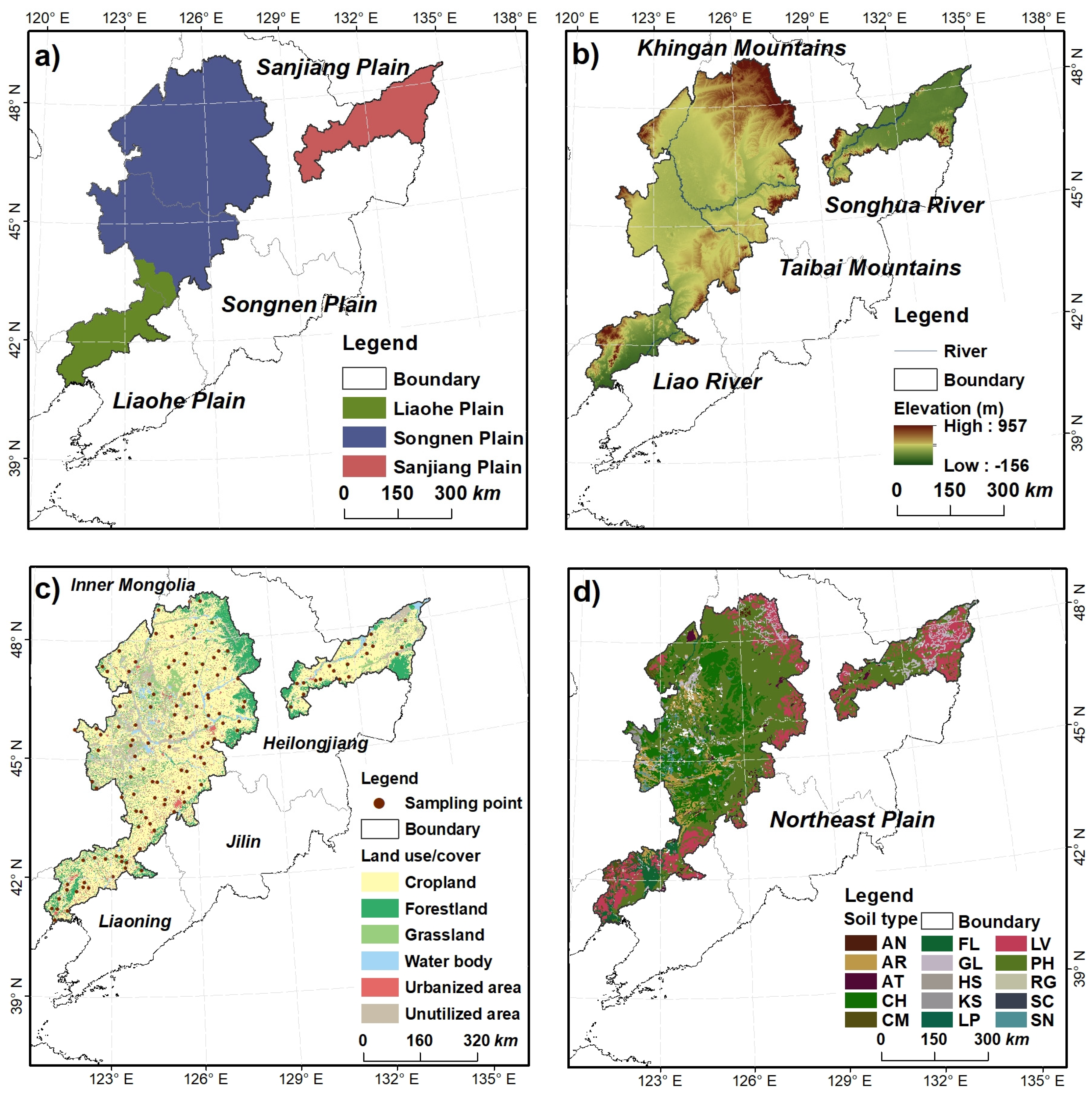
Figure 1. (a) Geographic location of the study area in Northeast Plain China; (b) elevation of the study area in Northeast Plain China; (c) spatial distribution of sampling points and land use/cover types of the study area in Northeast Plain China; (d) soil types of the study area in Northeast Plain China.
Remotesensing 15 05033 g001
Figure 2. Raincloud plot of SOC content in the plough layer and the compacted layer.
Remotesensing 15 05033 g002
Figure 3. Spatial distribution pattern at 90 m spatial resolution of uncertainty at the plough layer in (a) Northeast Plain, (b) Sanjiang Plain, (c) Songnen Plain, and (d) Liaohe Plain.
Remotesensing 15 05033 g003
Figure 4. Spatial distribution pattern at 90 m spatial resolution of uncertainty at the compacted layer in (a) Northeast Plain, (b) Sanjiang Plain, (c) Songnen Plain, and (d) Liaohe Plain.
Remotesensing 15 05033 g004
Figure 5. Relative importance of environmental covariates by QRF at the plough layer and the compacted layer, S&P is the soil and parent material covariate, C is the climate covariate, O is the organism covariate, R is the relief covariate, and N is the location covariate.
Remotesensing 15 05033 g005
Figure 6. Relative importance of detailed variables by QRF in (a) the plough layer and (b) the compacted layer, S&P is the soil and parent material covariate, C is the climate covariate, O is the organism covariate, R is the relief covariate, and N is the location covariate.
Remotesensing 15 05033 g006
Figure 7. Spatial distribution pattern at a 90 m spatial resolution of SOC at the plough layer in (a) Northeast Plain, (b) Sanjiang Plain, (c) Songnen Plain and, (d) Liaohe Plain.
Remotesensing 15 05033 g007
Figure 8. Spatial distribution pattern at a 90 m spatial resolution of SOC content at the compacted layer in (a) Northeast Plain, (b) Sanjiang Plain, (c) Songnen Plain, and (d) Liaohe Plain.
Remotesensing 15 05033 g008
Figure 9. Spatial distribution pattern at a 90 m spatial resolution of SOC difference between the plough layer and the compacted layer in (a) Northeast Plain, (b) Sanjiang Plain, (c) Songnen Plain and, (d) Liaohe Plain.
Remotesensing 15 05033 g009
Table 1. List of environmental covariates in the selected database.
VariableAbbreviationScaleCovariate a)Type b)PeriodReference
Soil erosionSE1000 mS&PQ2002–2016[27]
Silt contentSilt250 mS&PQ1960–2020[10,28]
Sand contentSand250 mS&PQ1960–2020[10,28]
Brightness indexBI30 mS&PQ2015–2017[25]
Bare soil indexBSI30 mS&PQ2015–2017[25]
Carbonate indexCarI30 mS&PQ2015–2017[25]
Gypsum indexGI30 mS&PQ2015–2017[25]
IsothermalityBIO031000 mCQ1970–2000[29]
Temperature seasonalityBIO041000 mCQ1970–2000[29]
Temperature annual rangeBIO071000 mCQ1970–2000[29]
Mean temperature of wettest quarterBIO081000 mCQ1970–2000[29]
Mean temperature of driest quarterBIO091000 mCQ1970–2000[29]
Mean temperature of warmest quarterBIO101000 mCQ1970–2000[29]
Mean temperature of coldest quarterBIO111000 mCQ1970–2000[29]
Precipitation of wettest monthBIO131000 mCQ1970–2000[29]
Daytime land surface temperatureLSTD1000 mCQ2002–2017[30]
Nighttime land surface temperatureLSTN1000 mCQ2002–2017[30]
Solar radiationSol1000 mCQ1970–2000[29]
Average temperatureTavg1000 mCQ1970–2000[29]
Maximum temperatureTmax1000 mCQ1970–2000[29]
Minimum temperatureTmin1000 mCQ1970–2000[29]
Vapor pressureVP1000 mCQ1970–2000[29]
The average of CANI in the crop periodCroCANIa30 mOQ2015–2017[25]
The average of NDRI in the non-crop periodNCroNDRIa30 mOQ2015–2017[25]
The average of GPP in the non-crop periodNCroGPPa500 mOQ2015–2017[31]
The average of NPP in the non-crop periodNCroNPPa500 mOQ2015–2017[31]
The average of FPAR in the non-crop periodNCroFPARa500 mOQ2015–2017[32]
The average of LAI in the non-crop periodNCroLAIa500 mOQ2015–2017[32]
The variance of GPP in the non-crop periodNCroGPPv500 mOQ2015–2017[31]
The variance of NPP in the non-crop periodNCroNPPv500 mOQ2015–2017[31]
ElevationELE90 mRQ2000[33]
Channel network base levelCNBL90 mRQ2000[33]
Valley depthVD90 mRQ2000[33]
Terrain wetness indexTWI90 mRQ2000[33]
Oblique geographic coordinate at 30°OGC3030 mNQ/[34]
Oblique geographic coordinate at 45°OGC4530 mNQ/[34]
Oblique geographic coordinate at 60°OGC6030 mNQ/[34]
Oblique geographic coordinate at 105°OGC10530 mNQ/[34]
Oblique geographic coordinate at 120°OGC12030 mNQ/[34]
Oblique geographic coordinate at 165°OGC16530 mNQ/[34]
a) Soil and parent material covariate (S&P), climate covariate (C), organism covariate (O), relief covariate (R), and position covariate (N). b) Quantitative variable (Q).
Table 2. Descriptive statistics for SOC content of 132 sampling points in Northeast Plain (g kg−1).
LayerMin1st QuMedianAverage3rd QuMaxSD%CVSkewnessKurtosis
SOC PL2.789.9514.9316.3320.7648.658.8053.881.124.56
SOC CL0.967.7512.0913.2117.4136.406.9952.910.723.19
SOC content in the plough layer (SOC PL), SOC content in the compacted layer (SOC CL), minimum (Min), maximum (Max), first quantile (1st Qu), third quantile (3rd Qu), coefficient of variation (%CV), standard deviation (SD), skewness (Skew), and kurtosis (Kurt).
Table 3. Performance of QRF on SOC predictions, assessed by R2 and RMSE of CV and OOB datasets, PICP of the CV dataset.
DepthOOBCVUncertainty
R2RMSE (g kg−1)R2RMSE (g kg−1)UPICP
PL0.615.450.685.101.050.88
CL0.544.750.584.641.090.86
Plough layer (SOC PL), compacted layer (CL), Quantile Regression Forest (QRF), out-of-bag (OOB), cross-validation (CV), coefficient of determination (R2), root mean square error (RMSE), prediction interval coverage percentage (PICP).
Disclaimer/Publisher’s Note: The statements, opinions and data contained in all publications are solely those of the individual author(s) and contributor(s) and not of MDPI and/or the editor(s). MDPI and/or the editor(s) disclaim responsibility for any injury to people or property resulting from any ideas, methods, instructions or products referred to in the content.