Abstract
Weather forecasting requires a comprehensive analysis of various types of meteorology data, and with the wide application of deep learning in various fields, deep learning has proved to have powerful feature extraction capabilities. In this paper, from the viewpoint of an image semantic segmentation problem, a deep learning framework based on semantic segmentation is proposed to nowcast Cloud-to-Ground and Intra-Cloud lightning simultaneously within an hour. First, a dataset with spatiotemporal features is constructed using radar echo reflectivity data and lightning observation data. More specifically, each sample in the dataset consists of the past half hour of observations. Then, a Light3DUnet is presented based on 3D U-Net. The three-dimensional structured network can extract spatiotemporal features, and the encoder–decoder structure and the skip connection can handle small targets and recover more details. Due to the sparsity of lightning observations, a weighted cross-loss function was used to evaluate network performance. Finally, Light3DUnet was trained using the dataset to predict Cloud-to-Ground and Intra-Cloud lightning in the next hour. We evaluated the prediction performance of the network using a real-world dataset from middle China. The results show that Light3DUnet has a good ability to nowcast IC and CG lightning. Meanwhile, due to the spatial position coupling of IC and CG on a two-dimensional plane, predictions from summing the probabilistic prediction matrices will be augmented to obtain accurate prediction results for total flashes.
1. Introduction
Lightning is one of the most common and disruptive natural weather phenomena, known for its strong localization, rapid development, and intense atmospheric conditions. Therefore, lightning prediction heavily relies on near-term forecasting based on observational data. Enhancing the accuracy of these near-term predictions remains a significant challenge in the field of weather forecasts [1,2,3,4,5].
Currently, the main method for lightning prediction is extrapolation based on real-time data collected from radar, satellite, and other sources, including TITAN [6], SCIT [7], optical flow techniques [8,9], and machine learning extrapolation [10,11]. Extrapolation models forecast lightning based on the motion features and trajectories of past observations. As more observations become available, it is difficult for extrapolation models to extract non-linear features and build models from the large number of high-spatial-resolution and high-temporal-resolution observations.
With the rapid development and widespread use of deep learning (DL), it has proven able to handle high-dimensional and complex spatiotemporal data, and demonstrates excellent modelling of non-linear problems. Because weather forecasting is essentially the processing of large amounts of spatial and temporal data from multiple sources of meteorological observation data, more and more researchers are applying DL to weather forecasting. In general, these DL-based forecasting methods can be divided into three categories, which are the recurrent neural network (RNN)-based structure, the convolutional neural network (CNN)-based structure, and their combined structure. For RNN-based structures, since long short-term memory (LSTM) networks have excellent ability in extracting temporal features, there are lots of methods presented [12,13]. For further extraction of spatial features, convolutional LSTM (convLSTM) is used in weather forecasting [14,15,16,17,18,19,20,21,22]. Such as Shi et al. proposed a convolutional long short-term memory (LSTM) network for precipitation nowcasting [14,15]. Geng et al. proposed LightNet+ based on ConvLSTM, which employed numerical models (WRF) and real-time lightning observations to predict lightning for the next 0–6 h [16,17]. CNN networks have advantages in extracting spatial features, but not well at temporal features. However, three-dimensional (3D) CNN networks can extract spatiotemporal features and work well. Therefore, Zhou et al. used multiple sources to construct 3D LightningNet based on SegNet, including satellite cloud images, radar reflectivity, and lightning density, and could provide a lightning probability forecast for the next 0–1 h [23]. Huang et al. proposed a deep learning model for short-term precipitation forecasting based on 3D CNN [24]. Additionally, the Pangu weather model is based on a 3D high-resolution global weather forecast system proposed by the Huawei Cloud Computing group [25].
However, there is no discussion to forecast Cloud-to-Ground (CG) and Intra-Cloud (IC) lightning simultaneously. IC is more responsive to the development of the lightning process. Therefore, from the viewpoint of image semantic segmentation [26,27,28,29,30], a deep learning framework for IC and CG nowcasting is presented in this paper. First, we construct a high-resolution dataset with spatiotemporal features based on radar reflectivity data and lightning data; second, for extracting the spatiotemporal features of the dataset, a Light3DUnet based on 3D U-Net is presented, which has a 3D CNN, an encoder-decoder architecture, and pathways between them. Then, Light3DUnet was trained using the past half hour observations to predict IC and CG lightning in the next one hour; finally, we demonstrate the effectiveness of this network for IC and CG forecasting using real data in middle China.
2. Materials and Methods
2.1. Data
2.1.1. Rader Data
The dataset for this study was provided by the China Next-Generation Weather Radar (CINRAD) network, which was deployed by the China Meteorological Administration (CMA). The CINRAD network is composed of 236 Doppler weather radars (including C-Band and S-Band radars) which are distributed across China. The study area in this paper is in the middle of China (112°–117°E, 28°–33°N); the radar reflectivity image products are operated by the radar with a 6 min frequency for a total of 240 scans per day, and cover a diameter of 240 km at 0.01° × 0.01° resolution, represented as 640 × 480 pixel image downloaded from the website of the CMA (http://data.cma.cn (accessed on 22 November 2022)). The dataset consists of two precipitation seasons (May to August) from 2018 to 2019, for a total of 59,040 maps.
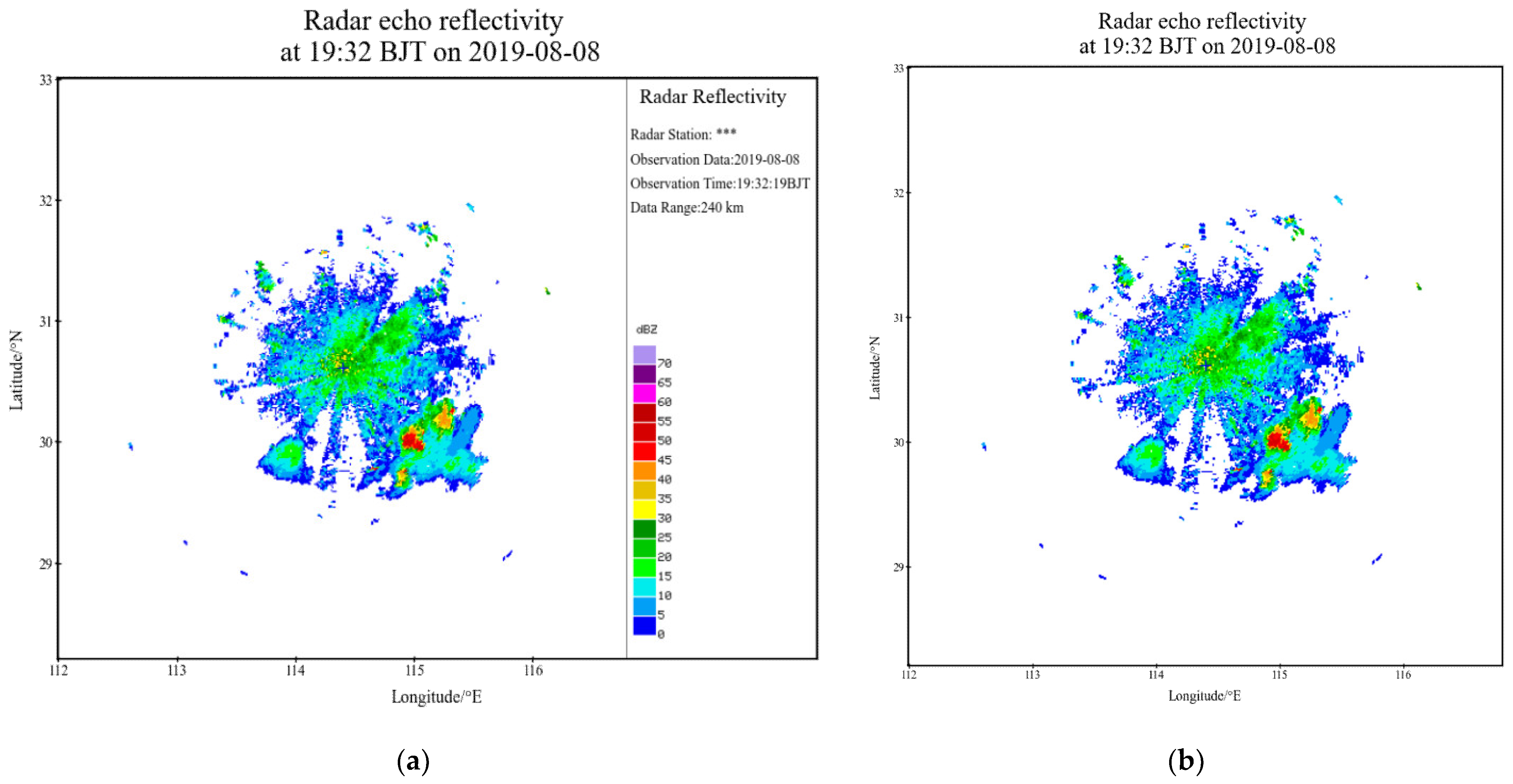
Due to some redundant information on the map, data cleaning is required, and the basic steps are the same as the [19], including removing the annotations (city name, river name, borderline, topography, e.g.,) from each map and filling in the related missing pixel values using the interpolation method. Figure 1 is the radar reflectivity at 19:32 BJT on 8 August 2019. Figure 1a gives the radar echo reflectivity after data cleaning. In this paper, however, the right side [481 × 0, 640 × 480] pixels of the map are cropped off, as that part is the description of the reflectivity map, including the name of radar station, the observation data and time, the data range and the legend, as shown in Figure 1a. After the data cleaning and image cropping, the final resulting figure is shown in Figure 1b. Finally, after processing all the radar reflectivity, the total samples are obtained at a size of 59,040 × 480 × 480.
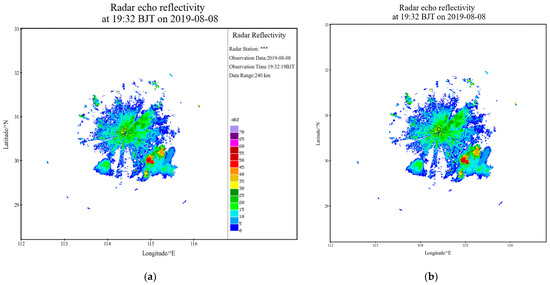
Figure 1.
Radar reflectivity at 19:32 BJT on 8 August 2019. (a) Radar echo reflectivity after data cleaning; (b) Final radar echo reflectivity after data cleaning and image cropping.
2.1.2. Lightning Data
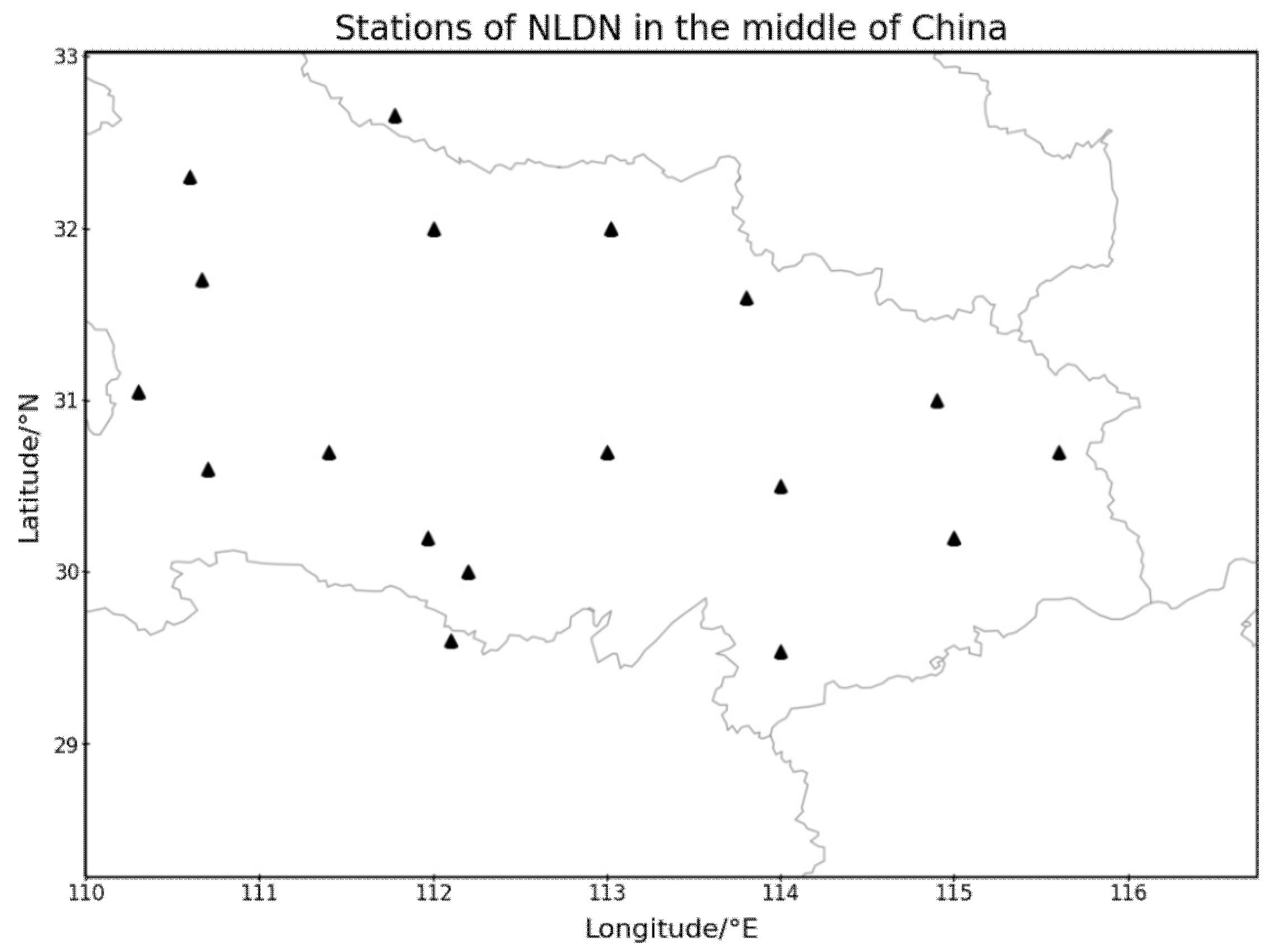
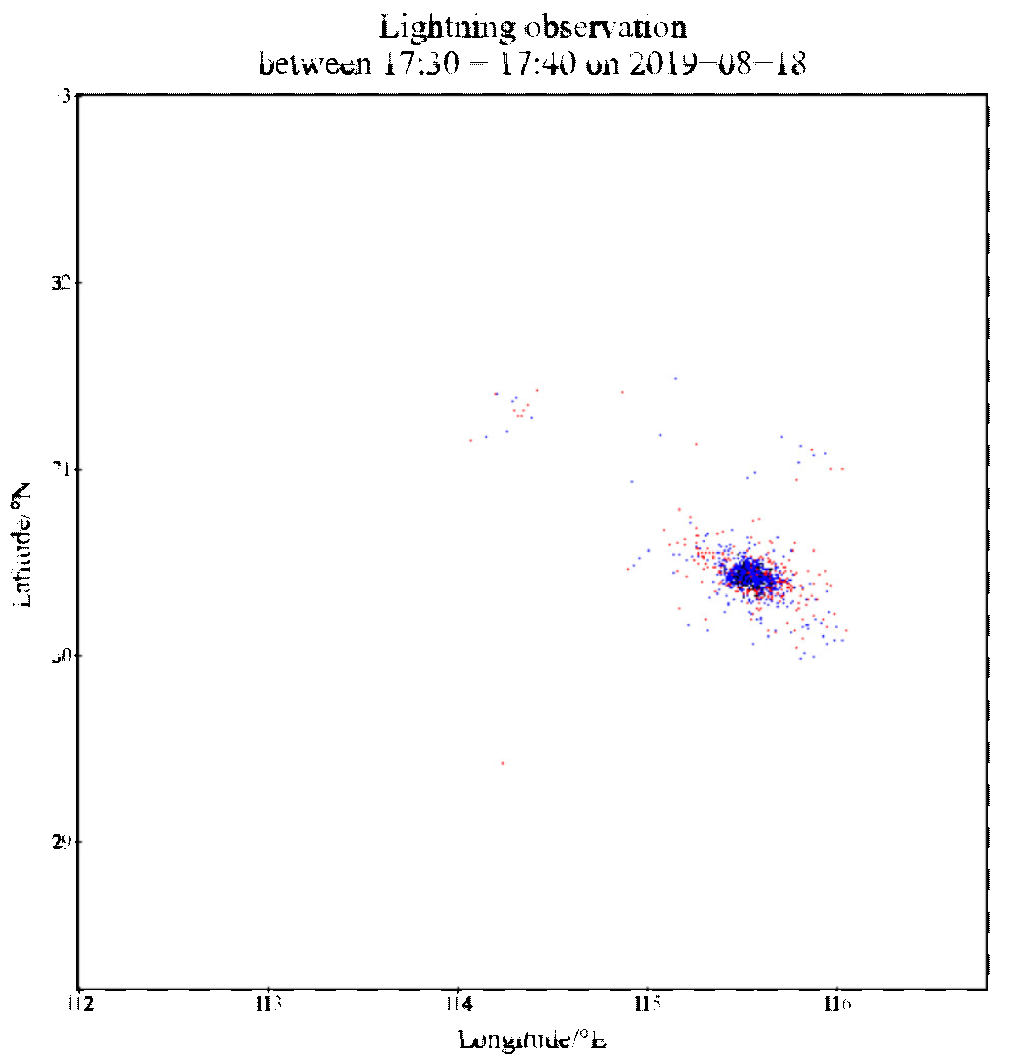
The lightning data used in this study were collected via the National Lightning Detection Network (NLDN) of China. This network can detect and measure the time, location, estimated current, flash polarity, and various other descriptors of individual lightning strikes including CG and IC. Figure 2 presents the distribution of the stations of NLDN in the middle of China. The detection efficiency and location accuracy of NLDN are larger than 90% and approximately 0.5 km for the studied area, respectively. To transform the raw data into a format compatible with our network, the individual CG and IC strikes are accumulated into maps of lightning density covering ten-minute periods, which are used as lightning observation images for the network. Figure 3 shows the lightning observation between 17:30–17:40 on 18 August 2019. The lightning strikes in the study area are projected onto the corresponding image’s two-dimensional grid according to their latitude and longitude, and CG and IC are accumulated one by one within 10 min and are denoted by red dots and blue dots, respectively.

Figure 2.
Distribution of the stations of NLDN in the middle of China. The black triangle denotes NLDN stations.
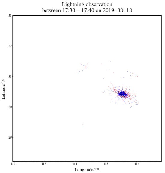
Figure 3.
Accumulating IC and CG lightning observations every 10 min; blue dots denote IC, and red dots denote GC.
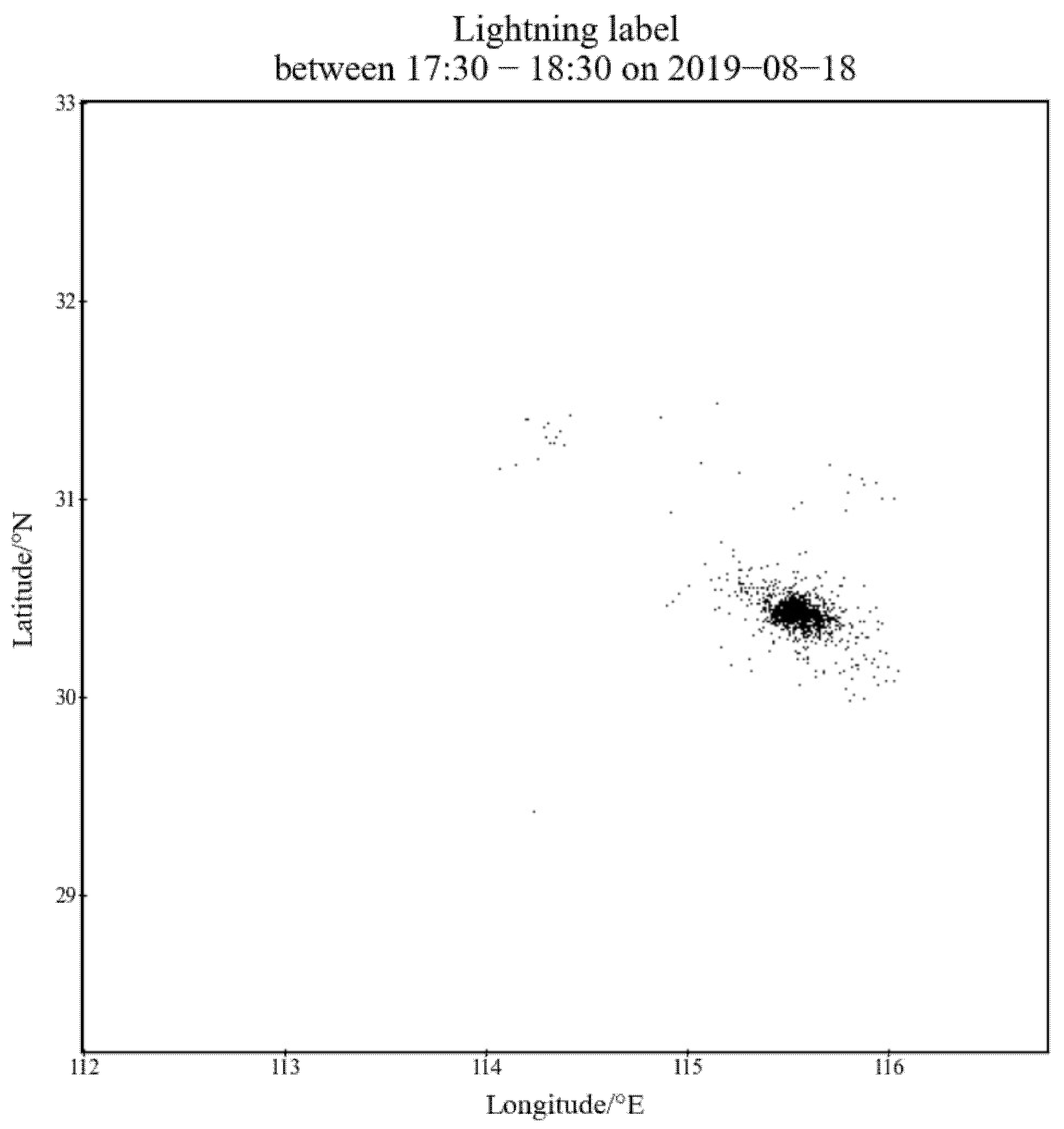
Furthermore, using the lightning data, the labels were created. As we not only discuss forecasting for CG but also for IC, there are two cases for which to generate a label. The first case is only forecasting for CG lightning. In this case, for the classification task, there are two classes: in one case, a CG event occurred, and in the other, no lightning event occurred. In particular, in this case, we treat IC as CG as well. Then, a pixel in the label is set to 1 if a CG/IC event occurred within the last hour; otherwise, it is set to 0. The second case involves forecasting for CG and IC, respectively. Therefore, there are three classes: CG event, IC event and no lightning event. A pixel in the label is set to 1 if an IC event occurred within the last one hour, set to 2 if CG occurred, and otherwise, is set to 0. Figure 4 shows that lightning label between 17:30–18:30 on 18 August 2019. Originally, the pixel values in the lightning labels should only be {0, 1} or {0, 1, 2}, but for illustration, here, we set the pixel value 0 to 255.
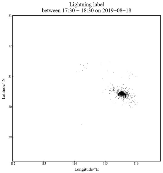
Figure 4.
Lightning labels based on the next hour. A pixel is set to 1 if an IC event occurred within the last one hour, set to 2 if CG occurred, and otherwise, is set to 255.
It must be noted that a total of 5485 total flashes occurred between 17:30–18:30 on 18 August 2019, including 2047 IC strikes and 3438 CG strikes. However, due to the spatial coupling of IC and CG and the lower temporal resolution, there are only 893 grids of IC and 1061 grids of CG on the lightning label for three classes, and 1954 grids of CG for two classes. Therefore, to make the most of the observed information, we generated a label every half hour.
2.1.3. Construction of the Dataset
As we aim to predict lightning, observed data are downselected from the period into the dataset such that only those data that showed convective activity were included. Obviously, for the fixed area, the more times lightning occurred in the same period, the more convective activity. Therefore, we identified these data based on the number of lightning strikes, which is set to 30. This means that the observations or labels created using the lightning data will be discarded as long as the accumulated number of lightning strikes is less than 30; in the corresponding periods of the one-to-one relationship between samples and labels, valid data can be downselected.
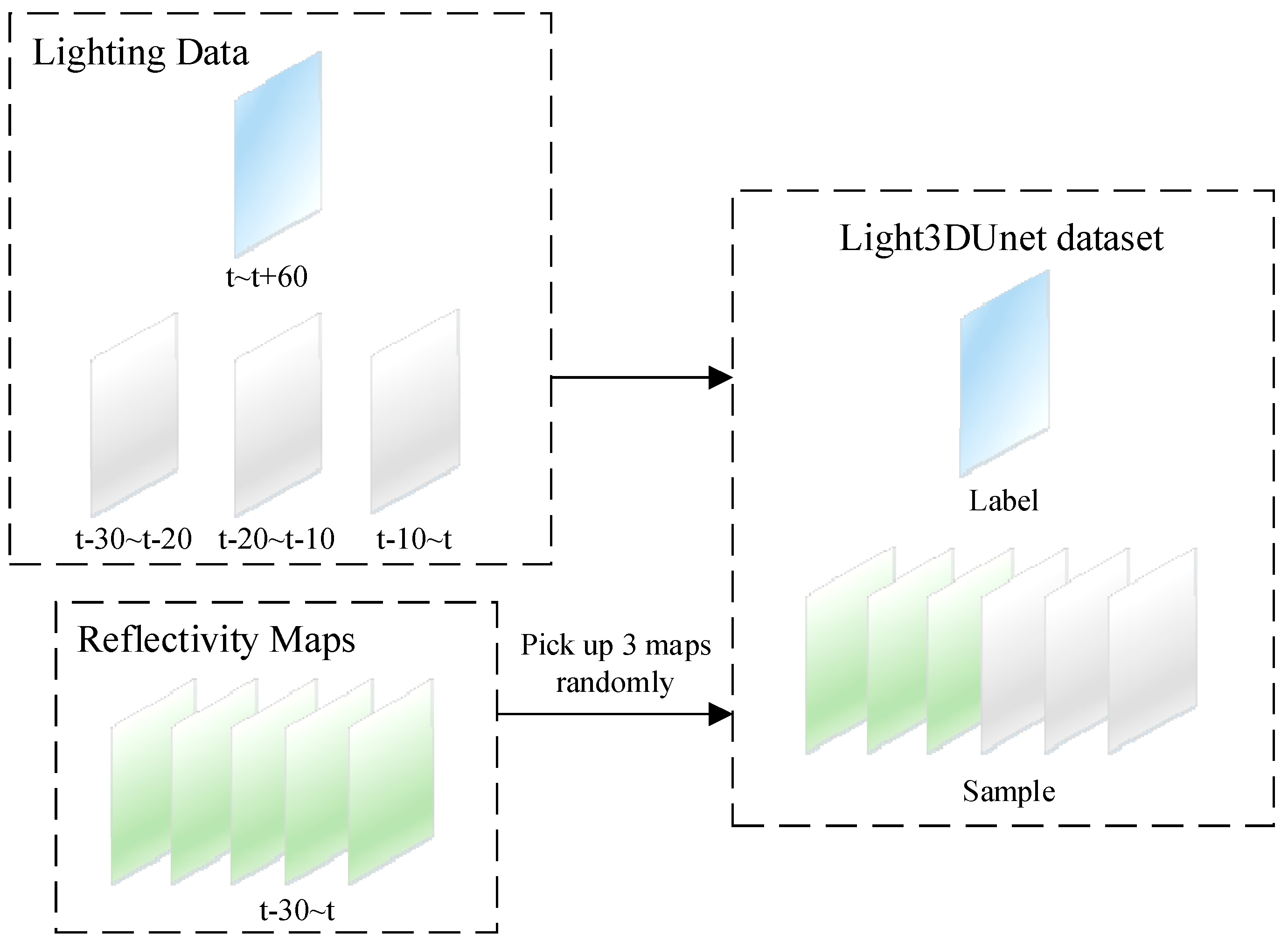
Then, we use the past 30 min of observation data to predict the lightning events within the next 0–60 min. For lightning observation, because it is generated at 10 min intervals, there are three images every 30 min. For radar reflectivity, as the radar has a 6 min frequency, there are five images every 30 min. Thus, we randomly picked three images from five maps. Additionally, labels are generated with each 30 min as the starting point and 60 min as the duration. So far, we have constructed a dataset with spatiotemporal properties for a three-dimensional segmentation network. Figure 5 shows an illustration of one sample label of the dataset. The final dataset for the three-dimension Light3DUnet is 1046 samples, each one being 6 × 3 × 480 × 480 size, where six is the number of maps and three is the channel of the maps.
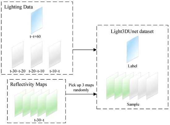
Figure 5.
Illustration of construction of the dataset for Light3DUnet.
2.2. Methodology
2.2.1. Neural Network
Due to the sparse, scattered, small-scale, and irregularly edged features of lightning observation images, semantic image segmentation is extremely challenging. The U-Net has an encoder–decoder structure and a pathway between them, and also has excellent detail retention and the ability to handle small, complex targets. U-Net is a two-dimensional network and can only extract two-dimensional spatial information. To extract both spatial and temporal information, a 3D U-Net has been proposed, and has proven to be extremely advantageous in medical semantic image segmentation [31].
For lightning segmentation, based on 3D U-Net, the Light3DUnet is presented to extract features in temporal and spatial dimensions in this paper. Similar to 3D U-Net, Light3DUnet has an encoder network and a corresponding decoder network, which takes 3D volumes as the input and processes them with corresponding 3D operations, in particular, 3D convolutions, 3D max pooling, and 3D up-convolutional layers. However, in Light3DUnet, because the size of the input 3D volumes was relatively small, the max pooling and up-convolutional layers should be modified based on the depth of input.
Figure 6 illustrates the network architecture. Light3DUnet has an encoder network and a decoder network, each with five resolution steps. In the encoder network, each layer contains two 3 × 3 × 3 convolutions with a padding of 1, each followed by a batch normalization (BN), then a ReLu, and then a 2 × 2 × 2 max pooling with strides of two in each dimension. Due to the inputs’ shape, the padding of the first max pooling is 1 × 0 × 0, and the others are 0 × 0 × 0. In the decoder network, each layer consists of an upsample, followed by two 3 × 3 × 3 convolutions each followed by a BN, then a ReLu. Particularly, the scale factor of the first upsample is 1 × 2 × 2, and of the second and third upsamples are 2 × 2 × 2; the output size of the final upsample is specified as 6 × 480 × 480. Shortcut connections from layers of equal resolution in the encoder network provide the essential high-resolution features of the decoder network. In the last layer, a 4 × 1 × 1 max pooling with a stride of 3 × 1 × 1 reduces the output depth to 1, followed by a 1 × 1× convolution that reduces the number of output channels to the number of labels, which is three in our case. Table 1 gives the details of the Light3DUnet. The architecture has 40,170,050 parameters in total, and has 40,162,114 trainable parameters.
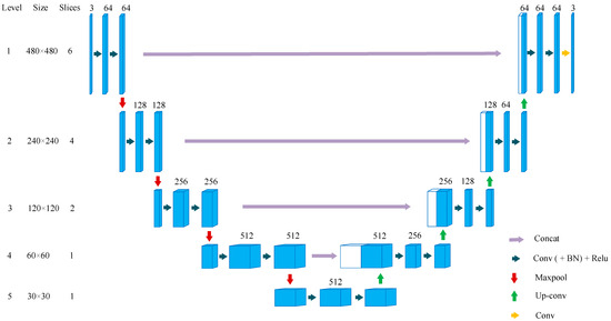
Figure 6.
Illustration of the framework of Light3DUnet.

Table 1.
The key configuration of Light3DUnet.
2.2.2. Model Training, Validation, and Testing
Due to there being huge numbers of trainable parameters, large numbers of samples are required to avoid overfitting. Therefore, dataset augmentation was used, for example, through random rotations at 90° intervals and random mirroring, to increase the diversity of the training samples. ADAM [32] is used as our optimizer, with a learning rate of 10−3. The cross-entropy loss is accepted, as it is popular in the classification task:
where N is the total number of pixels, i is the pixel, is the label on pixel i, is the probability of each pixel i, and c is the number of classes. means there are three classes; 0, 1, and 2 represent no lightning, IC, and CG, respectively. means there are two classes; 0 and 1 representing no lightning and lightning, respectively.
As the number of pixels in which lightning events occur is far less than that of pixels in which lightning events did not occur, the weighted cross-entropy loss is used in this paper to trade off the quantity gap between them. The final loss equation is given by the sum of the weighted cross-entropy loss:
where is the weight for class c. We empirically tune the weight and find that , for two classes, and , for three classes yields the best performance in our dataset.
The training was performed with four Nvidia Tesla V100 GPUs. The dataset is split into a test subset and a training subset. The test subset contained all the samples of June 2018 (199 samples), whereas the training set included the remaining samples (847 samples). A validation set, which was 15% of the training set, was randomly divided during the training. An early stopping strategy was used during the training. If the loss in the validation set has not improved for three epochs, the learning rate is divided by five. Additionally, if the loss has not improved for six epochs, the training is stopped. The model weight with the best validation loss is saved. The models output a three-channel matrix in which each grid point has a forecast probability obtained using the softmax classifier. We can turn them into deterministic forecasts by selecting a decision threshold T. Above T, it is predicted that lightning will occur; otherwise, non-occurrence is announced.
2.2.3. Evaluation
Four classical skill scores are used: probability of detection (POD), false alarm ratio (FAR), threat score (TS), and equitable threat score (ETS), to evaluate deterministic forecasts. Let N denote the total number of grid points. Let , , and represent the number of successful forecasts (prediction = 1, truth = 1), missing forecasts (prediction = 0, truth = 1), false negatives (prediction = 1, truth = 0), and correct negatives (prediction = 0, truth = 0), respectively. Then, we have
where , , and are determined by comparing the pre-defined threshold T, and r is the expectation of the number of lightning hits in random forecasts. By definition, for POD, TS, and ETS, larger is better, and for FAR, smaller is better.
3. Results
3.1. Skill Metrics
The skill scores are shown in Table 2, through which we compare Light3DUnet with DeepLabV3+ [29] using the validation dataset. To evaluate the validity of the spatiotemporal data, we discuss the dataset consisting solely of reflectivity and the dataset consisting of reflectivity echoes and lightning observations. Each sample in the dataset for Light3DUnet is 3 × 3 × 480 × 480 in size, constructed by the reflectivity echoes, and 6 × 3 × 480 × 480 in size, constructed by the reflectivity echoes and lightning observations, where the first 3/6 means that there are 3 or 6 maps, the second 3 means the channel of each map. Each sample in the dataset for DeepLabV3+ is 9 × 480 × 480 in size, constructed using the reflectivity, and 18 × 480 × 480 in size, constructed using the reflectivity and lightning observations, where 9 and 18 means there are 3 maps and 6 maps, respectively, and each map has 3 channels. The predefined threshold T described in Section 2.2 is set to 0.3 in Table 2. Obviously, the performance of lightning nowcast from Light3DUnet significantly outperforms that of DeepLabV3+. Additionally, the more input data used, the better the performance achieved.
Table 2.
Skill scores of two models on the validation set with the two different datasets.
For DeepLabV3+, even if more time information is provided, because the two-dimensional network cannot extract time-dimensional information, from Table 2, we can see that the performance of DeepLabV3+ is very poor. Moreover, when only the radar reflectivity is provided, DeepLabV3+ is invalid. As more data are provided, algorithm performance improves a bit.
For Light3DUet, the performance in forecasting CG and IC simultaneously is far better than that in forecasting CG alone. This is because since the areas of IC and CG events are usually very coincident, classifying three classes is equivalent to maximizing the use of lightning data labels to correct the neural network. At the same time, we find that the result of adding the probability matrices of IC and CG is good lightning nowcasting performance due to the high coincidence of the IC and CG regions. Table 2 shows the skill scores of the adding of the probability matrices of IC and CG. The pre-defined threshold T is 0.5 in Table 3. The performance using IC + CG is the best, as shown in Table 3.
Table 3.
Skill scores of the models on the validation set.
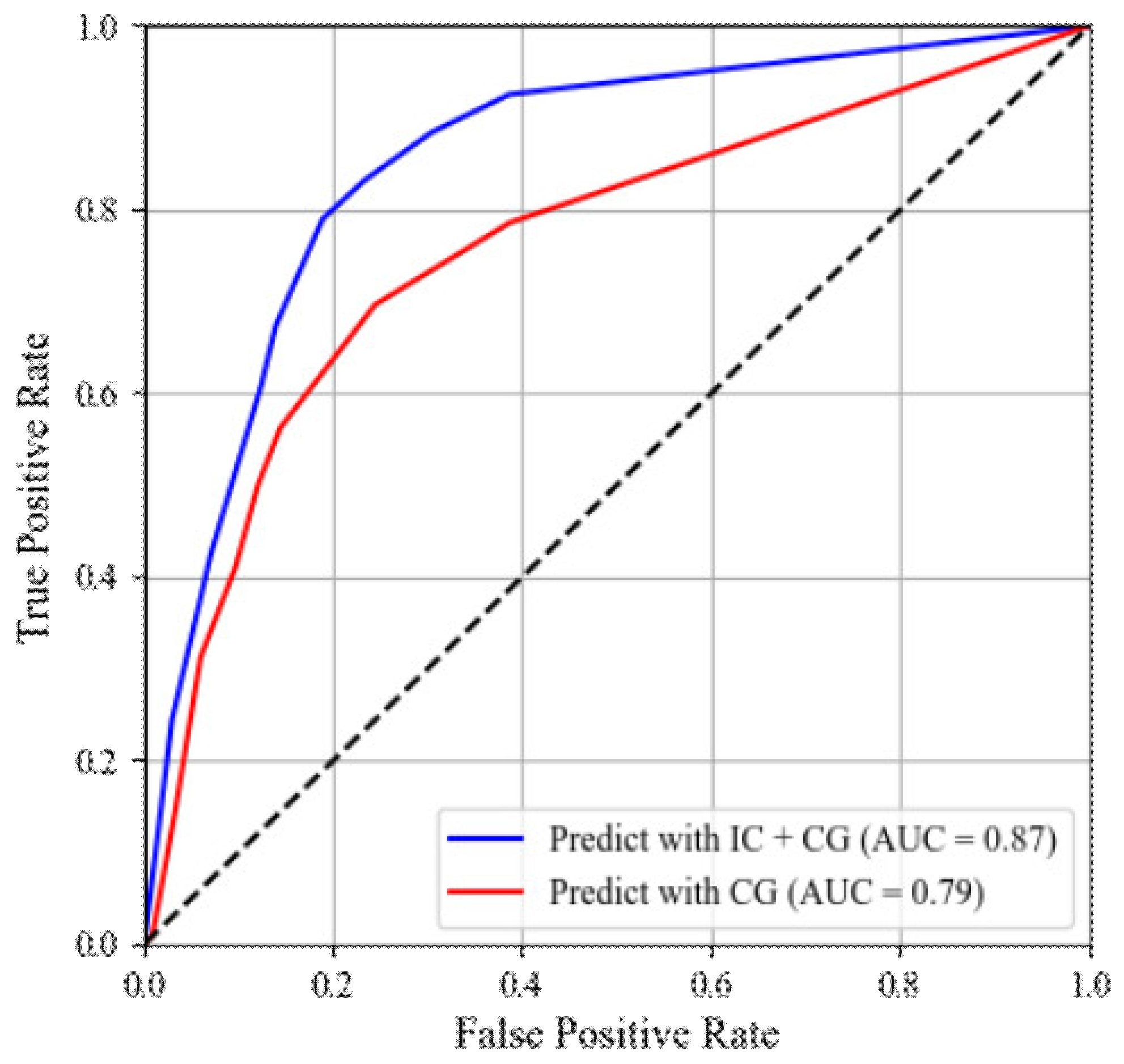
We also show the receiver operating characteristic (ROC) in Figure 7. The more efficient the method is, the closer the ROC curve is to the upper left corner. As with Table 2 and Table 3, we can see that the performance of Light3DUnet with IC + CG is better than with CG. The area under curve (AUC) is also consistent with Table 2 and Table 3, showing that the AUC of Light3DUnet with IC + CG is higher.
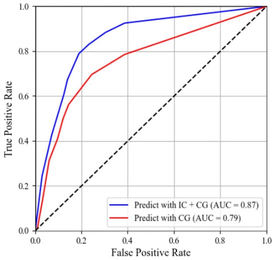
Figure 7.
ROC and AUC of lightning nowcasting for the next hour produced by Light3DUnet with different predicted class types for the validation dataset. True positive rate = and false positive rate = .
3.2. Case Study
Let us look at a lightning activity case that occurred on 2 August 2019, beginning at 13:00 BJT and ending at 20:00 BJT. The complete process of convection undergoes generating, developing, moving, merging, and splitting from its most vigorous stage at 15:00–17:00 BJT to weakening and dissipating at 20:00 BJT, with a duration of 8 h.
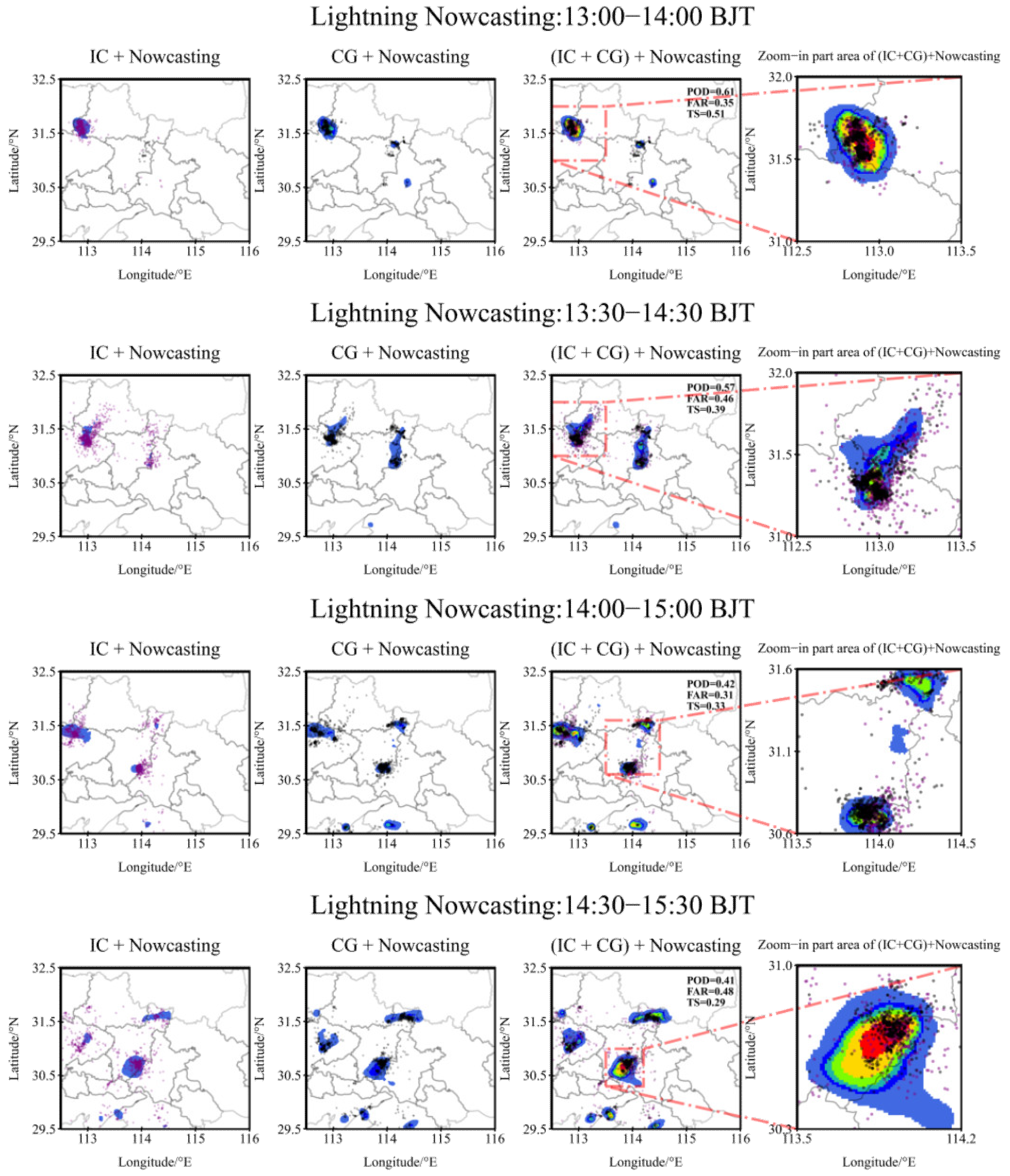
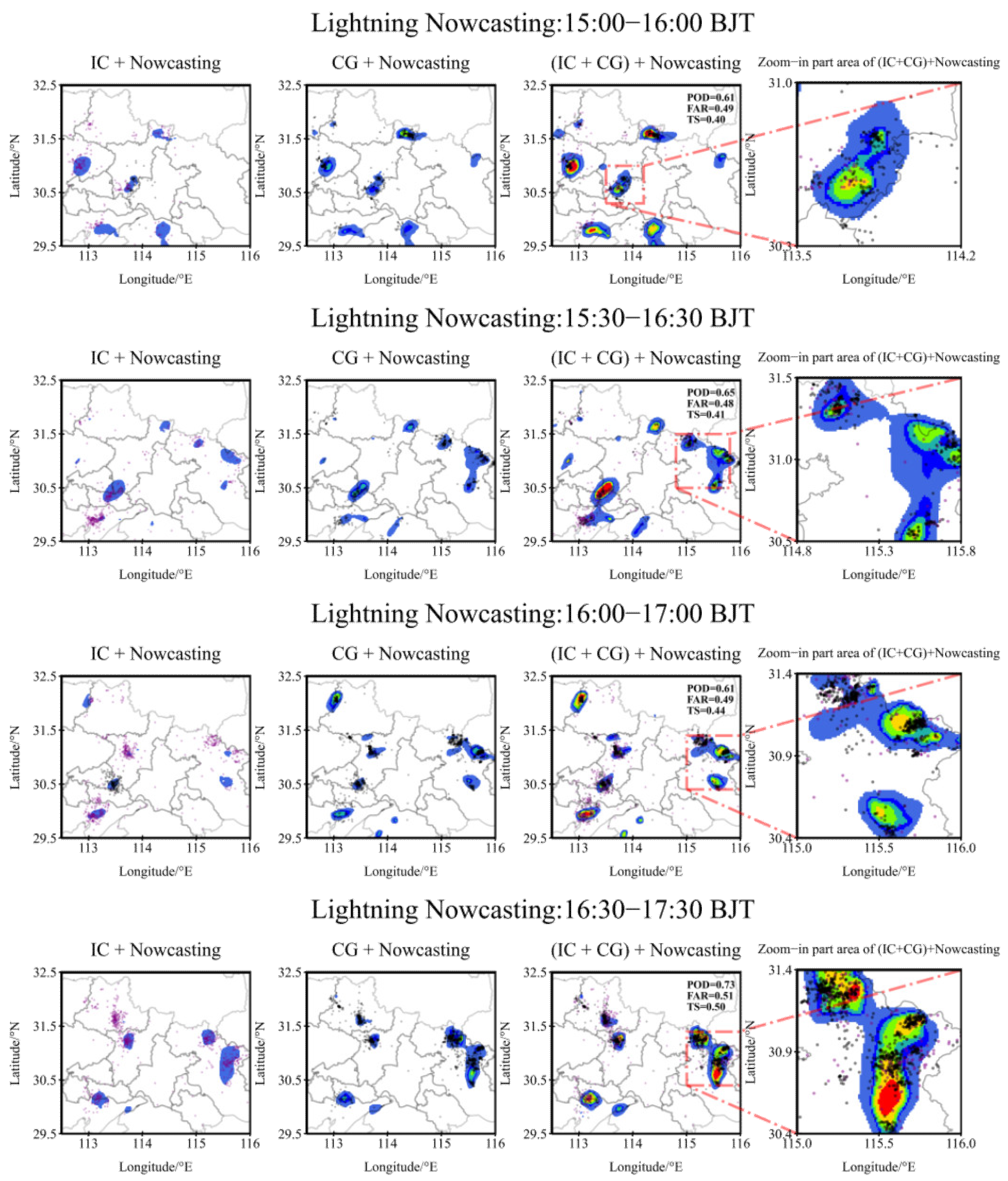
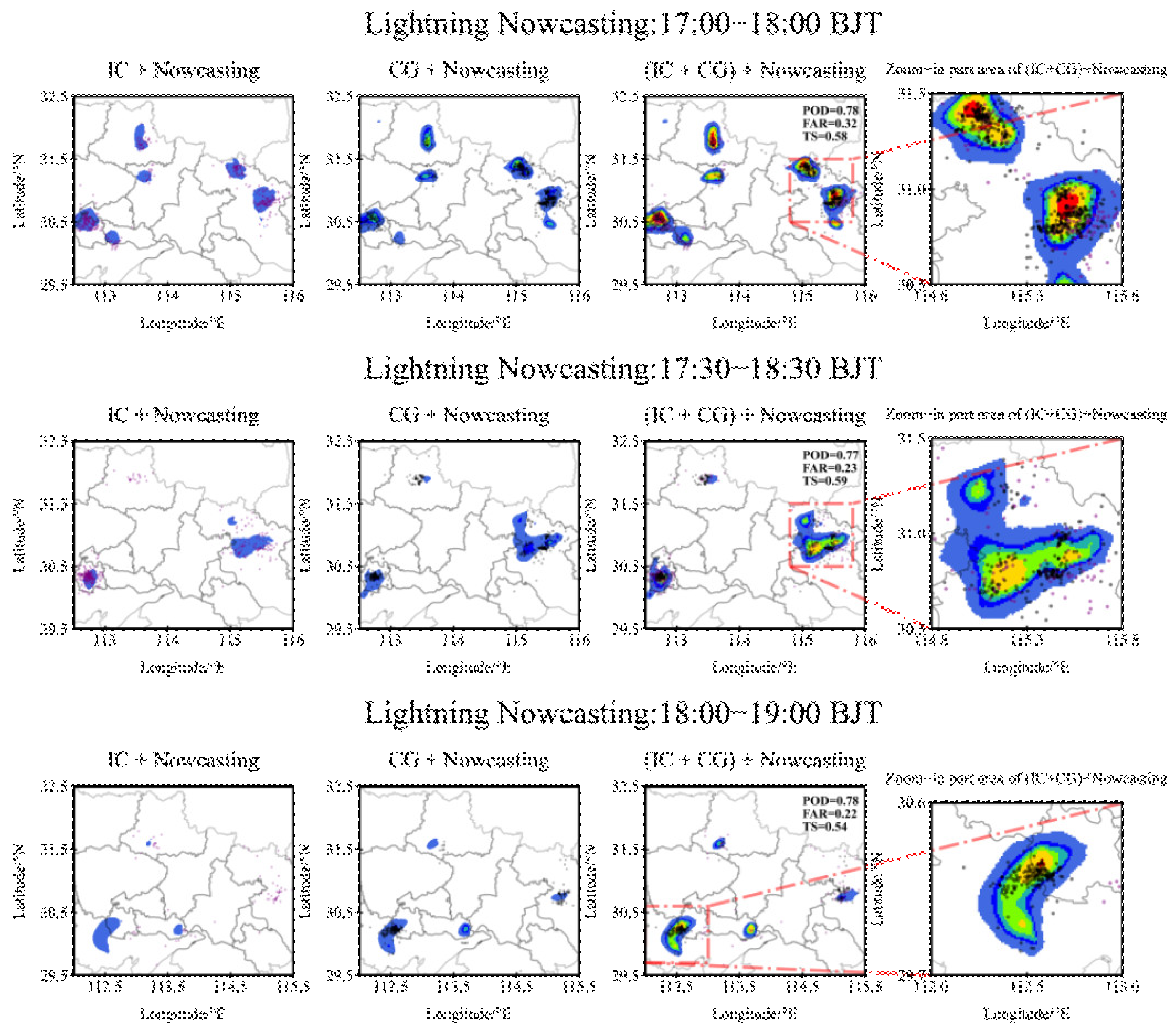
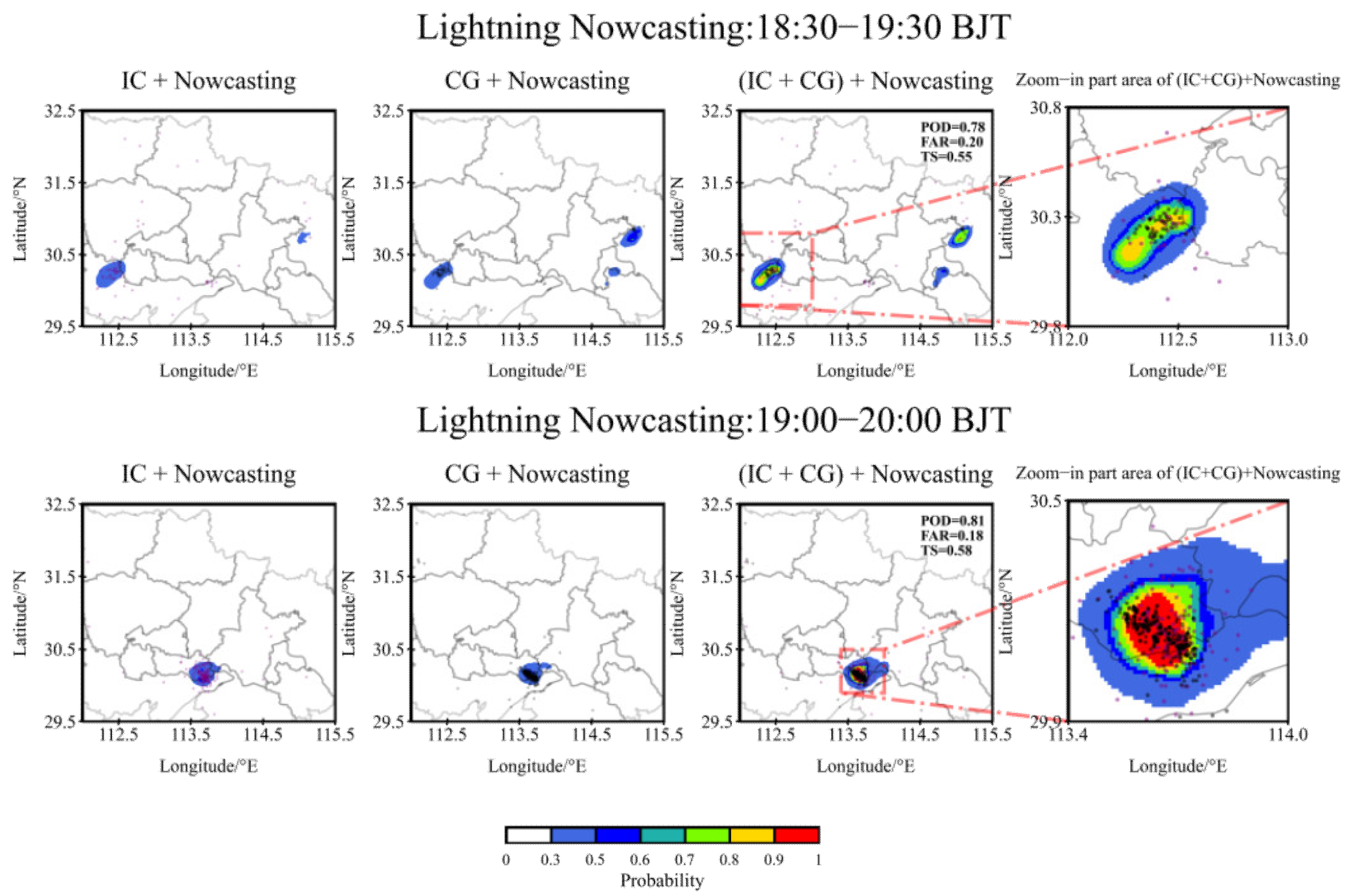
Figure 8 shows that the predictor outputs lightning nowcasting for the next hour every half hour, and each lightning nowcasting has four subfigures. The first one is the nowcasting probability of IC, and the second one is that of CG, respectively. The third is the lightning nowcasting produced by adding the probability predictor matrices of IC and CG, and the last one is the zoomed-in part area of the third subfigure. For illustrating the performance of nowcasting, lightning observations corresponding to the nowcasting are plotted in each subfigure, where the purple dots denote IC lightning strikes and the black dots denote CG lightning strikes. In the third subfigure, the POD, FAR, and TS, obtained by adding the probability matrices of IC and CG, are given on the top right corner.
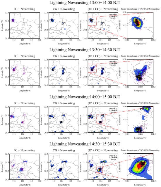

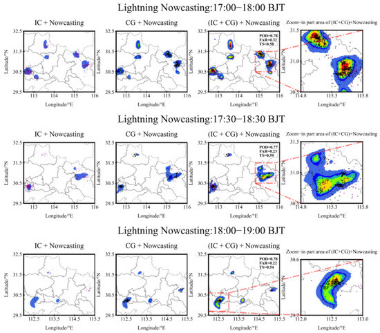

Figure 8.
The lightning nowcasting results for the next one hour from Light3DUnet and the corresponding lightning observations on 2 August 2019. Each lightning nowcasting has four subfigures, of which the first and the second are the probabilistic prediction of IC and CG obtained using the softmax classifier; the third and the last are the adding of the probabilistic prediction of IC and CG, from left to right. The purple dots and the black dots represent lightning observations of IC strikes and CG strikes.
From Figure 8, we can see that there were large-scale thunderstorm cells and two small-scale thunderstorm cells at 13:00–14:00 BJT. Over time, two small-scale thunderstorm cells merged into a large-scale one at 13:30–14:00 BJT, and split into two small ones at 14:00–14:30 BJT again. The convective systems of three original thunderstorm cells became more active, and three new convections were generated at 14:30–15:30 BJT. From 15:00–16:00 BJT to 17:00–18:00 BJT, the convective systems gradually developed eastward and reached the most vigorous stage. Then, the convective systems gradually weakened and finally disappeared after 17:00–18:00 BJT.
During the whole process of the thunderstorm, in Figure 8, the results show that Light3DUnet demonstrated an excellent performance in predicting lightning. The predicted thunderstorm cores and contour, whether IC or CG, or IC + CG, match very closely with the truth, meaning it successfully nowcast the movement, merging, splitting, weakening, and disappearance of thunderstorms. We can also see that, as analyzed in Section 2, IC and CG are spatially coupled. Due to this property, the prediction probability is increased in the coupled region. Obviously, the higher the probability is, the higher the lightning density is. Thus, the results of POD, FAR, and TS are sound.
To further evaluate the nowcasting performance of Light3DUnet, Figure 9 gives the lightning observations and lightning predictions for the next hour with the radar reflectivity of the prediction start time from 15:00 BJT to 17:30 BJT. Additionally, we focus on a specific area (114°–116°E, 30°–32°N). First, from Figure 9, the lightning predictions reflect both the radar reflectivity and the lightning observations, responding well to the radar reflectivity as well as the lightning observations, and successfully nowcasting the movement, merging, splitting, weakening, and disappearance of thunderstorms. Second, we find that Light3DUnet can forecast newborn convective systems. Observing the red dashed rectangle region in Figure 9, we can see that there is no indication in the radar reflectivity imagery of the initiation of the convective system at 15:00 BJT in Figure 9a; half an hour later, in Figure 9b, the prediction region in the red rectangle develops from one to two, in which the upper prediction region expands without any indication from the radar reflectivity, and a single convective system develops around the lower expected region. By 16:00 BJT in Figure 9c, it can be seen from the radar reflectivity imagery that convective systems start to trigger in the red rectangle; until Figure 9d, at 16:30 BJT, the radar reflectivity imagery indicates that lightning has already developed and matured in the red rectangle. From the whole process, it can be seen that Light3DUnet not only successfully forecasts the movement of the existing thunderstorm system, but also has a good prediction effect on the lightning initiation process. In this case, the algorithm can forecast the newborn convective system for more than 30 min.
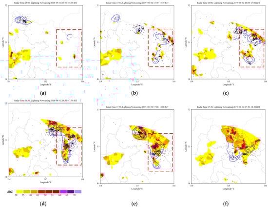
Figure 9.
The lightning nowcasting results for the next one hour from Light3DUnet, the corresponding radar reflectivity, and the lightning observations on 2 August 2019. The dots represent lightning observations, the contours show the lightning probabilistic nowcasting, which is the probabilistic of IC + CG, and the color-shaded areas are radar reflectivity. Radar reflectivity is retained only in the portion wherein intensity is greater than or equal to 30 dBZ, and the legend is consistent with Figure 1a. Each subfigure is the prediction result for the different periods, where the radar reflectivity is the start of the prediction period. (a) Lightning nowcasting for 15:00 to 16:00 BJT; radar reflectivity is at 15:00. (b) Lightning nowcasting for 15:30 to 16:30 BJT; radar reflectivity is at 15:30. (c) Lightning nowcasting for 16:00 to 17:00 BJT; radar reflectivity is at 16:00. (d) Lightning nowcasting for 16:30 to 17:30 BJT; radar reflectivity is at 16:30. (e) Lightning nowcasting for 17:00 to 18:00 BJT; radar reflectivity is at 17:00. (f) Lightning nowcasting for 17:30 to 18:30 BJT; radar reflectivity is at 17:30.
4. Discussion and Conclusions
This paper presents a deep learning framework (i.e., Light3DUnet) for nowcasting lightning of both IC and CG. We evaluated Light3DUnet on a real-world dataset which includes radar reflectivity and lightning data from Middle China. The experimental results demonstrate that Light3DUnet can effectively achieve IC and CG lightning nowcasts in the next hour. Especially, Light3DUnet showed a strong performance in nowcasting total flashes. This performance gain is attributed to three underlying ideas: effectively applied radar reflectivity and lightning data, the excellent detail retention ability of the Light3DUnet network, and enhancement of image segmentation results due to the spatial position coupling of IC and CG.
Firstly, the effective organization and construction of datasets based on different data sources are crucial for lighting forecasting. It has been confirmed by several investigations that the richer the data used for analysis, the more reliable the forecast results [15,16,22]. Due to the high accuracy of U-Net and the ability to retain detailed information when segmenting images, it is more advantageous when dealing with small targets and complex detailed images. The Light3DUnet proposed in this paper achieves good performance not only for large-scale lightning nowcasts, but also for rapidly developing, small-scale lightning nowcasts, as demonstrated in Table 3, Figure 7, Figure 8 and Figure 9. Besides, due to the location coupling of IC and CG, the summation of IC and CG probability predictions can be used to obtain more accurate probability prediction of total flashes. Moreover, Light3DUnet can forecast newborn convective systems for more than 30 min.
In this paper, the radar reflectivity image used is the processed two-dimensional product, which is the maximum reflectivity factor found in each elevation azimuth scan projected onto Cartesian grid points in a single scan. Similarly, the lightning observation data are the signal-processed products that provide the 2D location of lightning. In the next step, we will use the radar raw echo data and lightning observation raw signals, and utilize the three-dimensional information of the radar raw echo and the lightning observation raw signals to predict IC and CG lightning more accurately. Additionally, more data sources will be explored, such as satellite data, automatic weather station data, etc. We will discuss the performance of the proposed Light3DUnet on data from other regions and weather patterns not covered in the training dataset. Moreover, this paper explores the use of image segmentation networks to predict IC, GC, and total flashes. Based on this work, we will try to use other DL network models. Furthermore, we will also try to implement lightning forecasts for a range of 1–6 h.
Author Contributions
Conceptualization, L.F. and C.Z.; Data curation, L.F. and C.Z.; Formal analysis, L.F. and C.Z.; Funding acquisition, L.F.; Investigation, L.F. and C.Z.; Methodology, L.F. and C.Z.; Resources, L.F. and C.Z.; Software, L.F. and C.Z.; Validation, L.F. and C.Z.; Writing—original draft, L.F. and C.Z.; Writing—review and editing, L.F. and C.Z. All authors have read and agreed to the published version of the manuscript.
Funding
This research was funded by the High-Level Talent Project of Chengdu Normal University (No. YJRC2020-12), Key Laboratory of Featured Plant Development and Research in Sichuan Province (No. TSZW2110), Chengdu Normal University Scientific Research and Innovation Team (No. CSCXTD2020B09), Key Laboratory of Multidimensional Data Perception and Intelligent Information Processing in Dazhou City (No. DWSJ2201, DWSJ2209), Sichuan Provincial Department of Education’s Higher Education Talent Training Quality and Teaching Reform Project (No. JG2021-1389), Chengdu Normal University Teaching Reform Project (No. 2022JG23) and Chengdu Normal University Innovation and entrepreneurship training program for college students (No. 202214389031).
Data Availability Statement
The radar echo reflectivity data can be found at http://data.cma.cn and http://www.nmc.cn/publish/radar/chinaall.html (accessed on 22 November 2022).
Acknowledgments
The authors would like to thank the reviewers for their valuable suggestions that increased the quality of this paper.
Conflicts of Interest
The authors declare no conflict of interest.
References
- Lynn, B.H.; Yair, Y.; Price, C.; Kelman, G.; Clark, A.J. Predicting cloud-to-ground and intracloud lightning in weather forecast models. Wea. Forecast. 2012, 27, 1470–1488. [Google Scholar] [CrossRef]
- Gatlin, P.N.; Goodman, S.J. A total lightning trending algorithm to identify severe thunderstorms. J. Atmos. Ocean. Technol. 2010, 27, 3–22. [Google Scholar] [CrossRef]
- Stensrud, D.J.; Wicker, L.J.; Xue, M.; Dawson, D.T.; Yussouf, N.; Wheatley, D.W.; Thompson, T.E.; Snook, N.A.; Smith, T.M.; Schenkman, A.D.; et al. Progress and challenges with warn-on-forecast. Atmos. Res. 2013, 123, 2–16. [Google Scholar] [CrossRef]
- Farnell, C.; Rigo, T.; Pineda, N. Lightning jump as a nowcast predictor: Application to severe weather events in Catalonia. Atmos. Res. 2017, 183, 130–141. [Google Scholar] [CrossRef]
- Schultz, C.J.; Carey, L.D.; Schultz, E.V.; Blakeslee, R.J. Kinematic and microphysical significance of lightning jumps versus nonjump increases in total flash rate. Wea. Forecast. 2017, 32, 275–288. [Google Scholar] [CrossRef] [PubMed]
- Dixon, M.; Wiener, G. TITAN: Thunderstorm identification, tracking, analysis, and nowcasting—A radar-based methodology. J. Atmos. Ocean. Technol. 1993, 10, 785–797. [Google Scholar] [CrossRef]
- Johnson, J.T.; MacKeen, P.L.; Witt, A.; Mitchell, E.D.W.; Stumpf, G.J.; Eilts, M.D.; Thomas, K.W. The storm cell identification and tracking algorithm: An enhanced WSR-88D algorithm. Wea. Forecast. 1998, 13, 263–276. [Google Scholar] [CrossRef]
- Bechini, R.; Chandrasekar, V. An enhanced optical flow technique for radar nowcasting of precipitation and winds. J. Atmos. Oceanic Technol. 2017, 34, 2637–2658. [Google Scholar] [CrossRef]
- Woo, W.C.; Wong, W.K. Operational application of optical flow techniques to radar-based rainfall nowcasting. Atmosphere 2017, 8, 48. [Google Scholar] [CrossRef]
- Han, L.; Sun, J.; Zhang, W.; Xiu, Y.; Feng, H.; Lin, Y. A machine learning nowcasting method based on real-time reanalysis data. J. Geophys. Res. Atmos. 2017, 122, 4038–4051. [Google Scholar] [CrossRef]
- Leinonen, J.; Hamann, U.; Germann, U.; Mecikalski, J.R. Nowcasting thunderstorm hazards using machine learning: The impact of data sources on performance. Nat. Hazards Earth Syst. Sci. 2021, 22, 577–597. [Google Scholar] [CrossRef]
- Wang, Y.; Long, M.; Wang, J.; Gao, Z.; Yu, P.S. PredRNN: Recurrent neural networks for predictive learning using spatiotemporal LSTMs. In Proceedings of the 31st Conference on Neural Information Processing Systems, Long Beach, CA, USA, 4–9 December 2017. [Google Scholar]
- Shi, E.; Li, Q.; Gu, D.; Zhao, Z. A method of weather radar echo extrapolation based on convolutional neural networks. In Proceedings of the International Conference on Multimedia Modeling, Bangkok, Thailand, 5–7 February 2018. [Google Scholar]
- Shi, X.; Chen, Z.; Wang, H.; Yeung, D.Y.; Wong, W.K.; Woo, W.C. Convolutional LSTM network: A machine learning approach for precipitation nowcasting. In Proceedings of the 29th Conference on Neural Information Processing Systems, NeurIPS, Montreal, QC, Canada, 7–12 December 2015. [Google Scholar]
- Shi, X.; Gao, Z.; Lausen, L.; Wang, H.; Yeung, D.Y.; Wong, W.K.; Woo, W.C. Deep learning for precipitation nowcasting: A benchmark and a new model. In Proceedings of the 31st Conference on Neural Information Processing Systems, NeurIPS, Long Beach, CA, USA, 4–9 December 2017. [Google Scholar]
- Geng, Y.-A.; Li, Q.; Lin, T.; Jiang, L.; Xu, L.; Dong, Z.; Yao, W.; Lyu, W.; Zhang, Y. LightNet: A dual spatiotemporal encoder network model for lightning prediction. In Proceedings of the 25th ACM SIGKDD International Conference on Knowledge Discovery & Data Mining, Anchorage, AK, USA, 4–8 August 2019. [Google Scholar]
- Geng, Y.-A.; Li, Q.; Lin, T.; Yao, W.; Xu, L.; Dong, Z.; Zheng, D.; Zhou, X.-Y.; Zheng, L.; Lyu, W.-T.; et al. A deep learning framework for lightning forecasting with multi-source spatiotemporal data. Q. J. R. Meteorol. Soc. 2021, 147, 4048–4062. [Google Scholar] [CrossRef]
- Chen, L.; Cao, Y.; Ma, L.; Zhang, J. A Deep Learning-Based Methodology for Precipitation Nowcasting With Radar. Earth Space Sci. 2020, 7, e2019EA000812. [Google Scholar] [CrossRef]
- Yasuno, T.; Ishii, A.; Amakata, M. Rain-Code Fusion: Code-to-Code ConvLSTM Forecasting Spatiotemporal Precipitation. In Proceedings of the International Conference on Pattern Recognition, Virtual Event, 10–15 January 2021; Springer: Cham, Switzerland, 2021. [Google Scholar]
- Yao, G.; Liu, Z.; Guo, X.; Wei, C.; Li, X.; Chen, Z. Prediction of Weather Radar Images via a Deep LSTM for Nowcasting. In Proceedings of the 2020 International Joint Conference on Neural Networks (IJCNN), Glasgow, UK, 19–24 July 2020. [Google Scholar]
- Luo, C.; Li, X.; Wen, Y.; Ye, Y.; Zhang, X. A Novel LSTM Model with Interaction Dual Attention for Radar Echo Extrapolation. Remote Sens. 2021, 13, 164. [Google Scholar] [CrossRef]
- Ma, C.; Li, S.; Wang, A.; Yang, J.; Chen, G. Altimeter observation-based eddy nowcasting using an improved Conv-LSTM network. Remote Sens. 2019, 11, 783. [Google Scholar] [CrossRef]
- Zhou, K.; Zheng, Y.; Dong, W.; Wang, T. A deep learning network for cloud-to-ground lightning nowcasting with multisource data. J. Appl. Meteor. Climatol. 2020, 37, 927–942. [Google Scholar] [CrossRef]
- Huang, Q.; Chen, S.; Tan, J. TSRC: A Deep Learning Model for Precipitation Short-Term Forecasting over China Using Radar Echo Data. Remote Sens. 2023, 15, 142. [Google Scholar] [CrossRef]
- Bi, K.; Xie, L.; Zhang, H.; Chen, X.; Gu, X.; Tian, Q. Pangu-Weather: A 3D High-Resolution Model for Fast and Accurate Global Weather Forecast. arXiv 2022, arXiv:2211.02556. [Google Scholar]
- Shelhamer, E.; Long, J.; Darrell, T. Fully convolutional networks for semantic segmentation. IEEE Trans. Pattern Anal. Mach. Intell. 2017, 39, 640–651. [Google Scholar] [CrossRef]
- Badrinarayanan, V.; Kendall, A.; Cipolla, R. SegNet: A deep convolutional encoder-decoder architecture for image segmentation. IEEE Trans. Pattern Anal. Mach. Intell. 2017, 39, 2481–2495. [Google Scholar] [CrossRef]
- Ronneberger, O.; Fischer, P.; Brox, T. U-Net: Convolutional networks for biomedical image segmentation. Med. Image Comput. Comput.-Assist. Interv. 2015, 9351, 234–241. [Google Scholar]
- Chen, L.C.; Papandreou, G.; Kokkinos, I.; Murphy, K.; Yuille, A.L. DeepLab: Semantic image segmentation with deep convolutional nets, atrous convolution, and fully connected CRFs. IEEE Trans. Pattern Anal. Mach. Intell. 2018, 40, 834–848. [Google Scholar] [CrossRef] [PubMed]
- Chen, L.C.; Zhu, Y.; Papandreou, G.; Schroff, F.; Adam, H. Encoder-Decoder with Atrous Separable Convolution for Semantic Image Segmentation. In Proceedings of the European Conference on Computer Vision, Munich, Germany, 8–14 September 2018; p. 11211. [Google Scholar] [CrossRef]
- Çiçek, Ö.; Abdulkadir, A.; Lienkamp, S.S.; Brox, T.; Ronneberger, O. 3D U-Net: Learning Dense Volumetric Segmentation from Sparse Annotation. In Proceedings of the International Conference on Medical Image Computing and Computer-Assisted Intervention, Athens, Greece, 17–21 October 2016; p. 9901. [Google Scholar] [CrossRef]
- Kingma, D.; Ba, J. ADAM: A method for stochastic optimization. In Proceedings of the 3rd International Conference on Learning Representations, ICLR 2015, San Diego, CA, USA, 7–9 May 2015. [Google Scholar]


Disclaimer/Publisher’s Note: The statements, opinions and data contained in all publications are solely those of the individual author(s) and contributor(s) and not of MDPI and/or the editor(s). MDPI and/or the editor(s) disclaim responsibility for any injury to people or property resulting from any ideas, methods, instructions or products referred to in the content. |
© 2023 by the authors. Licensee MDPI, Basel, Switzerland. This article is an open access article distributed under the terms and conditions of the Creative Commons Attribution (CC BY) license (https://creativecommons.org/licenses/by/4.0/).