TCM-Net: Mixed Global–Local Learning for Salient Object Detection in Optical Remote Sensing Images

Abstract

Deep-learning methods have made significant progress for salient object detection in optical remote sensing images (ORSI-SOD). However, it is difficult for existing methods to effectively exploit both the multi-scale global context and local detail features due to the cluttered background and different scales that characterize ORSIs. To solve the problem, we propose a transformer and convolution mixed network (TCM-Net), with a U-shaped codec architecture for ORSI-SOD. By using a dual-path complementary network, we obtain both the global context and local detail information from the ORSIs of different resolution. A local and global features fusion module was developed to integrate the information at corresponding decoder layers. Furthermore, an attention gate module was designed to refine features while suppressing noise at each decoder layer. Finally, we tailored a hybrid loss function to our network structure, which incorporates three supervision strategies: global, local and output. Extensive experiments were conducted on three common datasets, and TCM-Net outperforms 17 state-of-the-art methods.

1. Introduction

Salient object detection (SOD) refers to the process of identifying and localizing visually attention-grabbing objects or regions within an image with pixelwise segmentation. These salient objects or regions have distinct visual features that can attract observers’ attention. By identifying objects or regions that effectively represent a scene, SOD plays a crucial role in complex visual tasks. As a result, it has been widely used in computer vision tasks such as image segmentation [1], video compression [2], object tracking [3] and quality assessment [4].

During the past decade, substantial progress has been made in SOD models designed for natural scene images (NSIs), with many algorithms proposed [5,6,7,8,9,10,11,12,13,14,15]. Given the crucial role that satellite and aerial remote sensing images play in various fields, such as agriculture [16] and disaster relief [17], researchers have begun exploring the potential utility of SOD techniques in optical remote sensing images (ORSIs).

It is natural that the mature NSI-SOD solutions will be considered for application to ORSI-SOD by researchers. In contrast to NSIs, ORSI-SOD is more challenging for several reasons: (1) ORSIs usually have a more complex background and a larger coverage area, resulting in more noise interference. (2) The size of salient objects appearing in ORSIs varies with the heights and angles of satellites and drones at different heights and angles. (3) Clouds and fog can cause noise during ORSI imaging, which significantly affects the image quality in remote sensing. Therefore, unsatisfactory performance often results from applying the NSI-SOD approach directly to ORSI-SOD. As shown in Figure 1d, even excellent NSI-SOD methods such as VSTNet [10], retrained on ORSIs, cannot fully highlight salient objects in these images.

In the last three years, several specific methods have been proposed for the ORSI-SOD task, and three public datasets have been constructed: ORSSD [18], EORSSD [19] and ORSI-4199 [20]. Nonetheless, the majority of these methods rely on a single convolutional neural network (CNN) despite their powerful capacity for extracting local detail features. CNN-based models typically necessitate a balance between global and local feature extraction structures, thereby making it difficult to model semantic interactions and contextual information directly. As shown in Figure 1c, CNN-based models perform feature down-sampling in the feature extraction process to reduce the amount of calculation, which easily causes small-scale features to be discarded.

The problem of how to deal with the local characteristics of a CNN and make the global features and local features work together has attracted the attention of many scholars. Related research includes increasing the width and depth of the network, the interaction of local and global information, the attention mechanism, multiscale feature expression and so on. For example, DAFNet [19] utilizes multiple layers of attention to guide shallow attention cues into deep layers and designed a global context-aware attention mechanism to capture long-range semantic context relationships. MJRBMNet [20] obtains global information through pyramid pooling (PPM) [21]. EMFINet [22] captures global context through a bridge module similar to the atrous spatial pyramid pooling (ASPP) [23]. These methods extract global information from local features obtained by CNNs, rather than encoding the global context directly. Therefore, it is difficult to extract clear global scene information from ORSIs with complex backgrounds.

Recently, the transformer model [24] has achieved significant success in the field of computer vision. This can be attributed to its ability to establish long-range dependencies using successive self-attention mechanisms. However, it lacks the capability to preserve the local details, resulting in ambiguous and coarse details of the final image. To address this issue, some approaches have introduced hybrid architectures that integrate both CNN and transformer models [25,26]. Unlike these methods, our approach uses a dual-path network structure that comprises a CNN and transformer to learn representations from both high and low resolutions. This allows for the full extraction of local and global features at varying scales, resulting in an optimal saliency map by fusing both types of features.

In this article, we propose a novel approach for the ORSI-SOD task, utilizing a CNN and transformer dual-path complementary architecture to extract local and global features from various resolutions. We designed a transformer and convolution mixer, and a U-shaped encoder–decoder network was applied to recover feature maps in order to generate accurate saliency maps. Within our framework, two key modules are proposed in the decoder module: the local and global feature fusion module (LGFF) and the attention gate (AG) module. The LGFF is used to incorporate context and detail information into the decoder layer, while the AG is designed to filter redundant information in ORSIs and reduce false predictions. Finally, a hybrid loss function that is tailored to the TCM-Net architecture was designed. The main contributions of our study are summarized as follows:

(1)

A novel approach is proposed for ORSI-SOD that combines the strengths of the CNN and transformer. Rather than a simple combination of two networks, the U-shaped codec network architecture can learn better representation by fusing and refining the features from local details and global contexts across different layers.

(2)

To comprehensively aggregate the global contexts and local details from encoder layers while reducing the redundancy of the multi-scale features, we propose the LGFF module and the AG module. In addition, we tailored a hybrid loss function that incorporates three supervision strategies, global, local and output, for enhanced representation learning.

(3)

Comparative experiments with 17 state-of-the-art SOD models on the common datasets of ORSSD [18], EORSSD [19] and ORSI-4199 [20] show that TCM-Net achieves the best performance.

The remaining parts of this article are organized as follows. In Section 2, we summarize the related works of NSI-SOD and ORSI-SOD. In Section 3, we elaborate on our TCM-Net. In Section 4, we present the experiments and ablation studies of our TCM-Net. Finally, the conclusion is drawn in Section 5.

2. Related Works

In this section, we review the classic works of NSI-SOD and ORSI-SOD, including traditional methods and CNN-based methods.

2.1. SOD Models in NSIs

(1)

Traditional Approaches: Over the past two decades, the theoretical system of SOD has undergone diversified development [27]. Itti et al. [28] proposed one of the earliest saliency models, which featured the well-known center-surround difference mechanism to locate salient objects. Since then, other models have emerged, such as the Kullback–Leibler divergence [29] and saliency tree [30]. In addition, hand-crafted features or visual priors, such as background prior [31], color histograms [32], color and brightness frequency-tuned detection [33] and color compactness [34], have been utilized to represent the saliency attribute of an object and generate bottom-up SOD models. However, these models have lower metrics or performance than deep-learning-based approaches.

(2)

Deep-Learning-Based Approaches: Recently, deep learning has achieved significant progress in SOD. Earlier deep-learning SOD models [35] utilized MLP classifiers to predict the saliency scores of deep features extracted from each image processing unit. A more effective and efficient approach is based on the full convolutional network (FCN) model [5,12,13], which uses the U-shaped network architecture with top-down feature encoding and skip connections to achieve semantic feature reuse at different levels. The attention mechanism has been widely applied to various computer vision tasks, including SOD. Liu [14] proposed a pixelwise contextual attention network for SOD by selectively focusing on contextual information of pixels. Meanwhile, the transformer model [24] has also been successful in global feature representation of SOD. Liu [10] proposed a visual saliency transformer for RGB and RGB-D SOD, and Xie [11] designed a pyramidal grafting network that combines a CNN and transformer to extract multi-scale features. These methods had achieved good results, but direct migration of NSI-SOD solutions to ORSI-SOD often resulted in unsatisfactory performance, and they still suffered from issues like blurred edges or inaccurate localization.

2.2. SOD Models in ORSIs

(1)

Traditional Approaches: Unlike a large number of traditional methods based on NSI-SOD, there are few works focusing on the ORSI-SOD. Zhao et al. [36] proposed a sparsity-guided saliency model that integrates saliency maps by incorporating global and background cues. Ma et al. [37] introduced a superpixel-to-pixel saliency model for detecting regions of interest based on texture and color features. Zhang et al. [38] aimed to determine the location of airports by integrating saliency results obtained from both vision-oriented and knowledge-oriented approaches. Zhang et al. [39] employed adaptive feature fusion of color, intensity, texture and global contrast using low-rank matrix recovery to generate the saliency map.

(2)

Deep-Learning-Based Approaches: Li et al. [18] first built the publicly available dataset called ORSSD for ORSI-SOD. Based on this work, Zhang et al. [19] extended the ORSSD dataset named EORSSD, containing some more challenging images, Tu et al. [20] also constructed the ORSI-4199 dataset with more complex scenarios and goals.Owing to the three public datasets, ORSI-SOD has received increasing attention [18,19,20,22,40,41,42,43,44,45,46]. Li et al. [18] introduced an end-to-end LV-Net for ORSI-SOD, which comprises a two-stream pyramid module and an encoder–decoder module. Zhou et al. [22] combined three strategies, namely image pyramid, feature pyramid and edge learning, to improve the performance of SOD. Cong et al. [41] is the first to explore the use of graph convolution networks for ORSI-SOD.

The aforementioned methods rely on CNN backbones, which may have limitations in capturing the overall context. Meanwhile, some approaches also incorporate transformer methods to address this issue. For example, HFANet [45] employs a hybrid architecture of CNNs and transformers for feature extraction, but the local features of the CNN may limit the effectiveness of the subsequent transformer structure for extracting image features. In addition, salient objects in ORSIs exhibit complex geometry structures, varying sizes and uncertain quantities and often encounter challenges such as occlusion, shadows and abnormal illumination. Therefore, there is a critical need to explore alternative methods that can effectively address these limitations and enhance the accuracy and robustness of the model.

3. Methodology

3.1. Architecture Overview

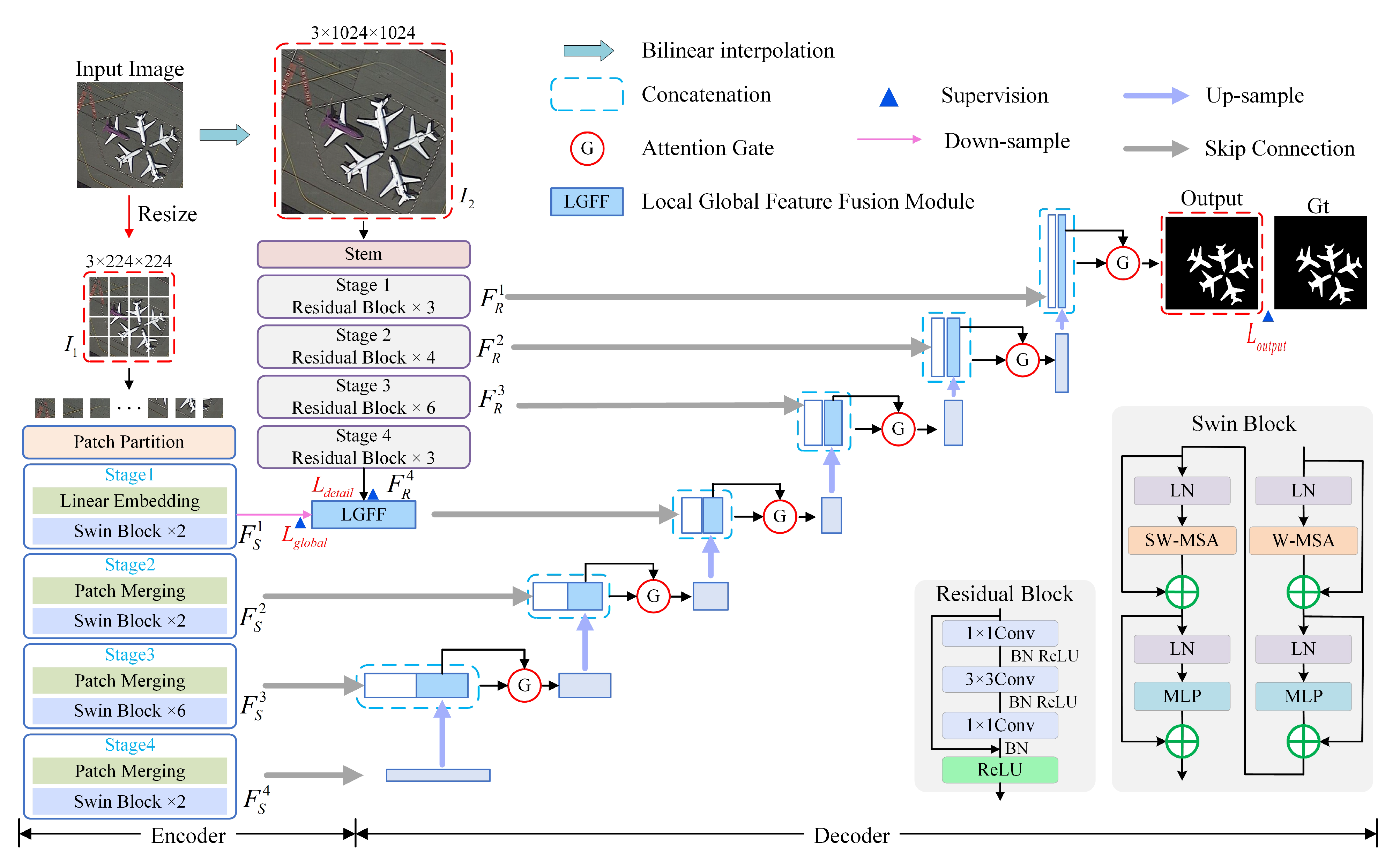
The proposed TCM-Net framework utilizes a U-shaped architecture that includes an encoder and a decoder, as shown in Figure 2. The encoder employs a dual-path complementary structure, incorporating a transformer branch and a CNN branch. Specifically, the CNN branch extracts local details, while the transformer branch captures global dependencies. The decoder aggregates global context and local details layer by layer. In detail, it conducts up-sampling on the encoded features, establishes skip connections between low-level and high-level features and filters out the redundant information through the AG module.

An input image I, can be resized into two images with different resolutions $I_1\in {\mathbb{R}}^{H_1\times W_1\times C}$ and $I_2\in {\mathbb{R}}^{H_2\times W_2\times C}$, where $H_1$ and $W_1$, $H_2$ and $W_2$ represent the height and width of low-resolution and high-resolution image, respectively, and both images have the same channel number denoted by C. The two images are input into the ResNet34 [47] and Swin transformer [48] networks, respectively. Then, we can obtain multi-scale local features $\{F_R^1,F_R^2,F_R^3,F_R^4|F_R^i\in \frac{H_1}{2^{i+1}}\times \frac{W_1}{2^{i+1}}\times (C\times 2^{i-1})|i=1,2,3,4\}$ and global features $\{F_S^1,F_S^2,F_S^3,F_S^4|F_S^i\in \frac{H_2}{2^{i+1}}\times \frac{W_2}{2^{i+1}}\times (C\times 2^{i+1})|i=1,2,3,4\}$. In the decoder, these features are integrated from the bottom-up by skip connections, up-sampling and the AG module to generate a precise saliency map.

3.2. Local and Global Feature Fusion Module (LGFF)

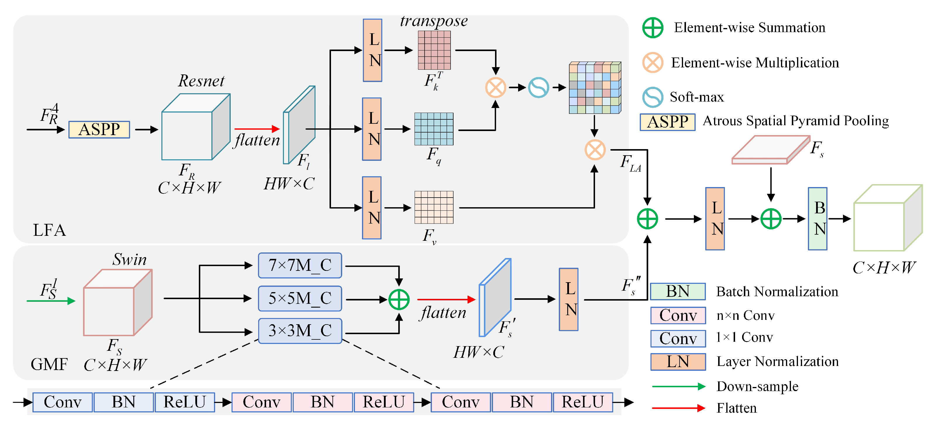
How to integrate global context and local details effectively represents an intriguing topic. Common approaches usually involve incorporating the pixelwise features and applying the corresponding convolution operation [6,14,15]. However, these methods are inadequate for capturing long-range dependencies. Therefore, we developed the LGFF module that consists of two sub-modules: the global feature multiscale fusion (GMF) and the local feature attention (LFA). These sub-modules enable efficient interaction between the global and local features, as shown in Figure 3.

Local feature attention (LFA): First, we utilized the Atrous Spatial Pyramid Pooling (ASPP) [23] layer to obtain a feature map with larger receptive field. ASPP employs atrous convolutional layers with various dilation rates to extract features at multiple scales. Subsequently, the attention scores are then generated by using pixel similarity. Finally, a weighted feature map can be obtained based on the attention scores. By assigning higher attention scores to the boundaries of salient objects associated with local details, the LFA can effectively reduce the impact of blurred boundaries caused by shadows or occlusions in ORSIs.

Specifically, the local feature $F_R^4$ is passed through the ASPP layer, producing a feature map $F_R\in {\mathbb{R}}^{C\times H\times W}$. Secondly, a feature matrix $F_l\in {\mathbb{R}}^{HW\times C}$ is formed. Lastly, $F_l$ is obtained by flattening $F_R$. Following this, $F_q$, $F_k$ and $F_v$($F_q$, $F_k$, $F_v\in {\mathbb{R}}^{HW\times C}$) is produced by applying three linear transformations with layer normalization (LN) to $F_L$, respectively. In terms of the self-attention mechanism, the attention score map $A\in {\mathbb{R}}^{HW\times HW}$ is formulated as:

$$A_{i,j}=softmax(F_q\times F_k^T)=\frac{\exp (F_{q,i},F_{{}_{k,j}}^T)}{{\displaystyle \sum _{i=1}^{W\times H}}\exp (F_{q,i},F_{{}_{k,j}}^T)}$$

(1)

The attention score map A is then matrix multiplied with the features map $F_v\in {\mathbb{R}}^{HW\times C}$ to obtain the weighted spatial feature map $F_{LA}$, which is given by:

$$F_{LA}=\eta \sum _{i=1}^{W\times H}{A}_{i,j}{F}_v$$

(2)

where $\eta$ is a learnable parameter. In this way, each spatial feature map $F_{LA}$ selectively aggregates the global context into the learned features, guided by the spatial attention map.

Global multi-scale feature fusion (GMF): Although the Swin transformer can effectively extract global contextual information, it is slightly insufficient for capturing local details and structural information due to its hierarchical design. To extract richer multi-scale detail information, this paper proposes a global multi-scale feature fusion module that simultaneously performs convolutions at several different scales. Specifically, we designed a multi-scale convolution block (M_C), which combines the feature information extracted by three different scales of M_C to obtain features with different receptive field sizes, thus enhancing detail features while speeding up the convergence of the model, which is formulated as follows:

$$\begin{array}{c}{F}_s^{i,1}=BR\left(u{p}_{\times 2}^{(2i+1)\times (2i+1)}\left(BR\left(u{p}_{\times 2}^{(2i+1)\times (2i+1)}\left(BR\left(dow{n}_{\times 4}^{i\times i}\left(F_s^1\right)\right)\right)\right)\right)\right),i=1,2,3\end{array}$$

(3)

$${F_s}^{″}=Linear(Flatten\left(BN\left(F_s^{11}\right)\right)+BN\left(F_s^{21}\right)+BN\left(F_s^{31}\right)))$$

(4)

where $dow{n}_{\times j}^{i\times i}$ denotes the j-fold down-sampling operation using convolution of size $i\times i$, and similarly $u{p}_{\times j}^{i\times i}$ denotes the j-fold up-sampling operation using convolution of size $i\times i$. BR denotes the BN layer and ReLU activation layer, and $Flatten$ denotes the straightening operation and layer normalization.

Following the two sub-modules LFA and GMF, the global feature output ${F_s}^{″}$ and the local feature output $F_{LA}$ are were added at the pixel level to obtain the new hybrid feature $F_f\in {\mathbb{R}}^{HW\times C}$. This hybrid feature is first restored to the dimensions of the input feature and then passed through an LN layer and added pixelwise to the original global feature $F_s^1\in {\mathbb{R}}^{C\times H\times W}$ to obtain the new feature, after which the final fused feature output ${F_f}^{″}$ is obtained through a BN layer and a ReLU layer, which is formulated as follows:

$${F_f}^{″}=\mathrm{ReLU}\left(BN({F_s}^{\prime }+LN(F_{LA}+{F_s}^{″}))\right)$$

(5)

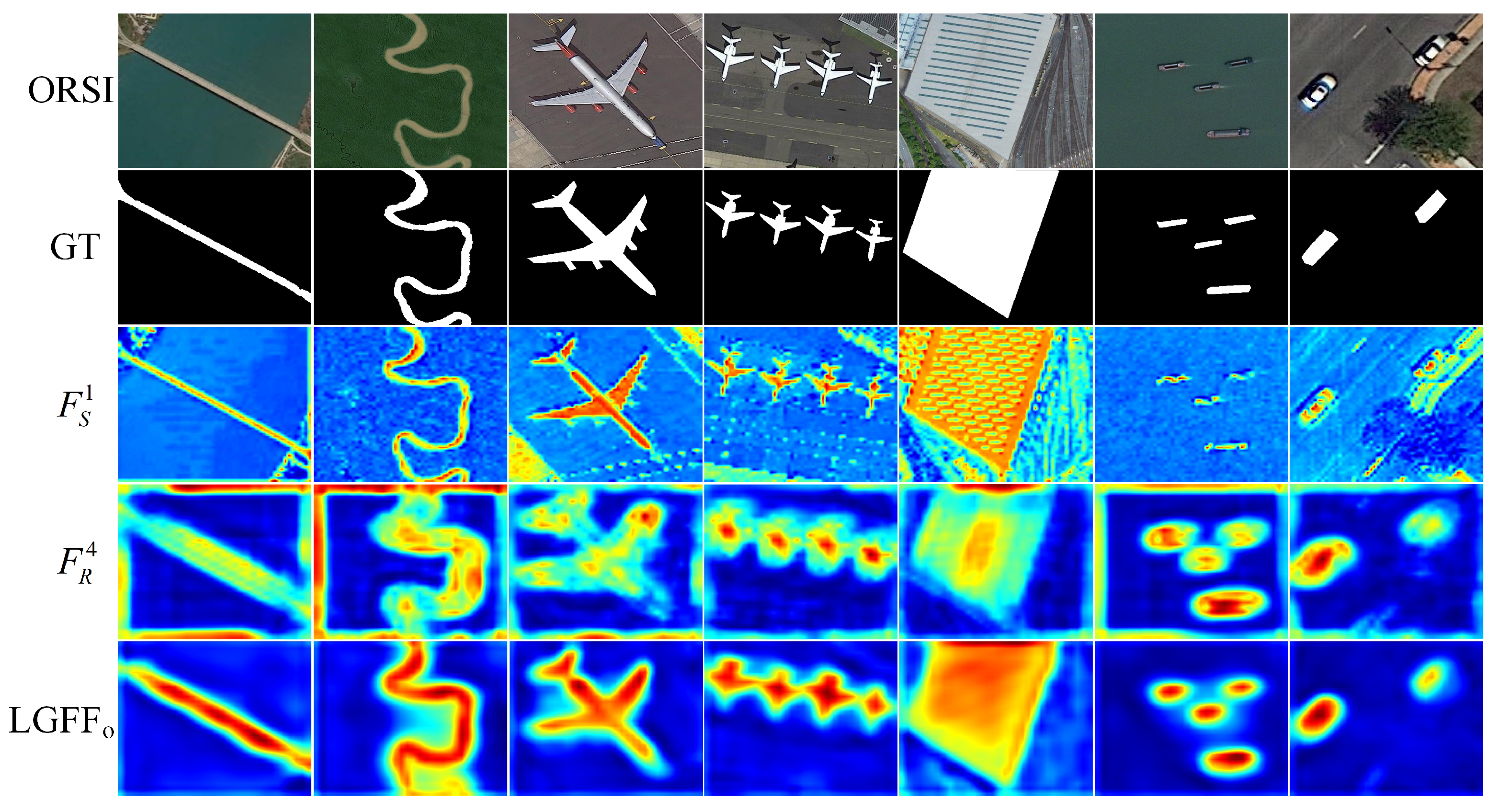
After using the LGFF module to fuse information of $F_S^1$ and $F_R^4$, Figure 4 shows the feature visual comparison of our LGFF module to both. It is apparent that our model effectively combines local and global information while preserving local details and global contextual information. This results in a more accurate and detailed feature representation, consequently enhancing the model’s detection capabilities.

3.3. Attention Gate (AG) Module

To improve the feature extraction and reduce redundant information, an AG module was developed. The module utilizes the information extracted from the coarse scale as input, eliminating irrelevant and noisy responses from skip connections. Unlike the single gate structure proposed in [49], our AG module includes two sub-gates: a spatial gate and a channel gate, as shown in Figure 5. The spatial gate regulates the spatial information of the fused and up-sampled features, suppressing irrelevant background information at different decoding stages. Meanwhile, the channel gate dynamically recalibrates the weights for each channel.

Specifically, the concatenation features and the up-sampling feature dimensionality are first reduced to the same channel dimension using 3 × 3 convolution and 1 × 1 convolution, respectively, both followed by BN and ReLU to obtain $F_c$ and $F_u$. Secondly, $F_c$ is combined with $F_u$ by element-wise addition to obtain the fused feature $F_a\in {\mathbb{R}}^{C\times H\times W}$. The resulting feature is then mapped to the [0, 1] range using the ReLU activation function. Next, the feature is further reduced using a 1 × 1 convolution to obtain $F^{\prime }\in R^{1\times H\times W}$. Finally, the corresponding location attention map P is computed by softmax normalization, which is formulated as follows:

$$P_{i,j}=\frac{\exp \left(F_{i,j}^{\prime }\right)}{{\displaystyle \sum _{i=1}^{H\times W}}\exp \left(F_{i,j}^{\prime }\right)}$$

(6)

where $P_{i,j}\in {\mathbb{R}}^{H\times W}$ denotes the feature similarity between the i-th pixel and the j-th point in the feature map. Finally, the attention map P is multiplied with the merged reduced-dimensional feature $F_a$, and the attention information of the current decision $F^{\prime }$ is guided by the merged feature $F_a$ to obtain the attention feature $F_P$ that is more accurate compared to the original concatenation feature position, which is formulated as follows:

$$F_P=\partial \sum _{i=1}^{H\times W}\sum _{j=1}^{H\times W}{P}_{i,j}\times F_a$$

(7)

where ∂ denotes the spatial scale factor, initialized to 0, and larger weights are obtained by continuous learning.

In the channel gate, average-pooling and max-pooling operations are performed separately on the fused feature $F_a\in {\mathbb{R}}^{C\times H\times W}$. Both pooled results are passed through a 3 × 3 convolution layer to learn cross-channel interactions. The resulting obtained channel attention weights are then mapped to the [0, 1] range using the sigmoid function. After that, the cross-channel attention weights obtained from different pooling operations are element-wise multiplied by the fused feature $F_a$ at each pixel, resulting in the corresponding channel attention with different pooling. Finally, the final channel feature $F_a^{\prime }$ is obtained by adding the matrix representations of these attention results together. The formulation of this process is as follows:

$$F_a^{\prime }=F\times \sigma (Con{v}_{3\times 3}\left(GAP\left(F_a\right)\right)+F\times \sigma (Con{v}_{3\times 3}\left(GMP\left(F_a\right)\right)$$

(8)

where $\sigma$ denotes the sigmoid activation function. $GAP$ and $GMP$ denote the operations of obtaining global information through global Avg pooling and global Max pooling, which can be expressed as:

$$G_k=\frac{1}{W\times H}\sum _{w=1}^W\sum _{h=1}^H{F}_k(w,h)$$

(9)

where $F_k(w,h)$ represents the feature map of $F_a$ on the k-th channel and spatial location $(w,h)$, while $G_k$ represents the global information of the feature map obtained by global average pooling and global max pooling on the k-th channel. The overall flow of our AG module can be defined as follows.

$$F_{AG}=\lambda F_P+F_a^{\prime }$$

(10)

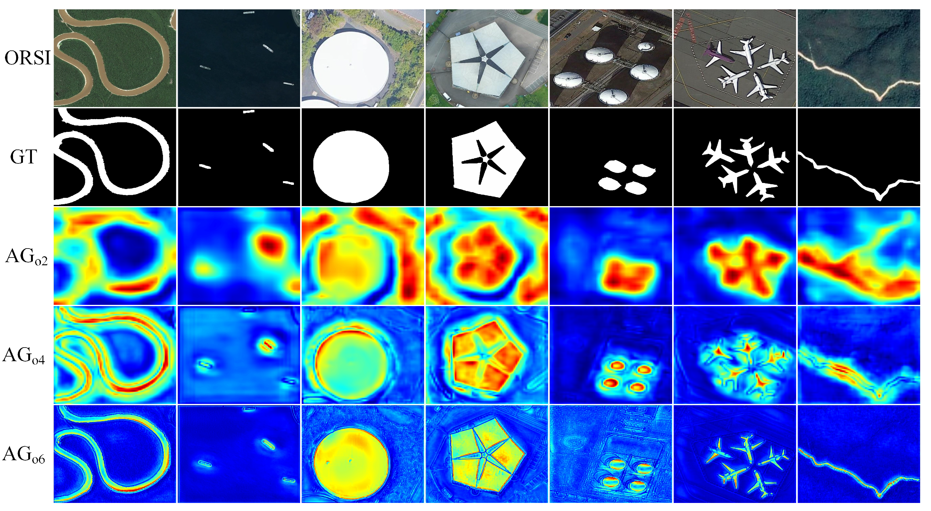
where $\lambda$ is a learnable parameter with an initial value of 1. Figure 6 shows the visualization of the bottom-up feature output of AG modules in various decoding layers. This illustrates the gradual suppression of redundant information and enhancement of feature representation. Our model produces accurate saliency maps by decoding each layer’s feature.

3.4. Loss Function

As shown in Figure 2, during the training process, we partitioned the mixed loss functions into three components: detail loss ($L_{detail}$), global loss ($L_{global}$) and final output loss ($L_{output}$), aiming for efficient convergence. These loss functions include pixel-level, map-level, structural similarity and F-metric with boundary information. The $L_{output}$, $L_{global}$ and $L_{detail}$ are supervisory functions for the last decoded feature output, S1 and R4, respectively.

$$\left\{\begin{array}{c}{l}_{bce}=-({\displaystyle \sum _{(x,y)}}g(x,y)log\left(p\right(x,y\left)\right)+{\displaystyle \sum _{(x,y)}}(1-g(x,y\left)\right)log(1-p(x,y\left)\right))\hfill \\ l_{iou}=1-\frac{{\displaystyle \sum _{(x,y)}}p(x,y)·g(x,y)+1}{{\displaystyle \sum _{(x,y)}}\left(p\right(x,y)+g(x,y)-p(x,y)·g(x,y)+1}\hfill \\ l_{ssim}=1-\frac{(2{\mu }_p{\mu }_g+C_1)(2{\sigma }_p{\sigma }_g+C_2)}{({\mu }_p^2+{\mu }_g^2+C_1)({\sigma }_p^2+{\sigma }_g^2+C_2)}\hfill \\ l_{fm}=1-F_{\beta }(pre,gt)\hfill \end{array}\right.$$

(11)

where BCE loss [50] is the most widely used loss function in SOD. The IoU loss [51] is a function that measures the overlap between predicted and ground truth labels. It penalizes differences to improve the model’s attention to object position and shape. SSIM loss [52] measures the structural similarity between two images. ${\mu }_p$, ${\mu }_g$, ${\sigma }_p$ and ${\sigma }_g$ are the mean and standard deviation of the predicted image and GT, respectively, $C_1,C_2$ are usually set to ${0.01}^2$ and ${0.003}^2$ to avoid the denominator of the function being 0. The metric perceptual loss F-m loss [53] is adapted from the metric commonly used in SOD, and we hope that its use will result in a high metric score for the predicted image. The total loss $L_{total}$ can be written as:

$$L_{total}=\delta ·L_{detail}+\varpi ·L_{global}+L_{output}$$

(12)

where parameters $\delta$ and $\varpi$ are used to balance the contributions of the three loss functions, and we set both of them to 0.2. Specifically, we incorporated edge information into the $L_{detail}$, and the edge data we used are derived from the Canny algorithm [54].

$$L_{detail}=\sum _{(edge,gt)}(l_{bce}+l_{iou}+l_{ssim})$$

(13)

By utilizing pixelwise, map-level and structural similarity loss functions, $L_{detail}$ is robust to local shape and boundary noise. This allows the $L_{detail}$ to supervise the structural information of the image, ensuring accurate edge prediction. For the global and prediction loss, we set the following functions.

$$L_{global}=l_{bce}+l_{iou}+l_{fm}$$

(14)

Among them, considering the global nature of $L_{global}$, we exclude the use of the structural similarity SSIM loss. To achieve a higher f-measure score, we incorporated the f-measure loss to supervise the global information, offset the imbalance between positive and negative samples and drive the convergence of the final prediction map.

To improve the accuracy of saliency detection, we utilized a joint supervision approach for the $L_{output}$. This approach incorporates four loss functions to balance global and local supervision, comprehensively considering the model’s performance in different aspects. Moreover, this approach enhances the model’s robustness, allowing it to perform effectively across diverse scenarios and datasets. By utilizing joint supervision during network training, we achieve a balanced weighting of the four loss functions, resulting in a more stable model.

$$L_{output}=l_{bce}+l_{iou}+l_{fm}+l_{ssim}$$

(15)

4. Experiments

4.1. Experimental Settings

(1)

Datasets: To fully validate our model, we conducted an extensive comparison of three public benchmark ORSI datasets.

ORSSD [18] is a dataset that includes 800 ORSIs, depicting significant objects, each accompanied by its corresponding ground truth. Of these, 600 images are used for training, and the remaining 200 images are reserved for testing.

EORSSD [19] is an extension of ORSSD, which includes 2000 more comprehensive and diverse scenes ORSIs with the corresponding GT. It consists of 1400 images as the training subset and the other 600 images for testing.

ORSI-4199 [20] is the latest and most challenging ORSI-SOD dataset. The dataset contains a total of 4199 images and the corresponding GTs, of which 2000 images are used for training and the remaining 2199 images are used as a test subset. In addition, it defines nine different scene attributes, which helps us to objectively evaluate the SOD models with various attributes.

(2)

Experimental details: Our model was implemented using PyTorch on a machine comprising an Intel(R) Core(TM) i9-10900X 3.70 GHz × 20 CPU, 128 GB of RAM (Kunshan, Jiangsu, China) and an NVIDIA GTX 2080Ti GPU (Suzhou, Jiangsu, China). The encoder was optimized using ResNet-34 [47] pre-training weights from PyTorch and Swin transformer [48] pre-training weights from Swin-B_224. The proposed TCM-Net can be trained end-to-end, and the network is optimized using Adam’s algorithm [55]. The maximum learning rate was set to 0.03 for the Swin backbone and 0.03 for the remaining components. During training, the learning initially increased and then decayed, with momentum set to 0.9 and weight decay to 0.001. The batch size was set to 8. Furthermore, during the training phase, each training image was resized to 1024 × 1024 and 224 × 224. The high-resolution images were input into the ResNet34 branch, while the low-resolution images were input into the Swin transformer branch. Due to the small size of the ORSSD dataset, we applied a strategy based on random flipping and rotation described in [18,19], which produced seven additional variants of the original training data to obtain a training set of 4800 training images. Then, three datasets were enhanced by cropping and multi-scale input images.

4.2. Evaluation Metrics

To quantitatively compare different saliency models for ORSSD, EORSSD and ORSI-4199 datasets, we adopted the following five evaluation metrics: the precision–recall (PR) curve [33], the F-measure curve, the max F-measure ($F_{\beta }^{\max }$) [33], the S-measure ($S_m$) [56] and the mean absolute error (MAE) [57].

Precision and recall are standard metrics to evaluate the model performance. The precision and recall scores can be calculated by comparing the binary mask to the ground truth.

F-measure is calculated as the weighted sum average of precision and recall, defined as follows:

$$F_{\beta }=\frac{(1+{\beta }^2)\times Precision\times Recall}{{\beta }^2\times Precision\times Recall}$$

(16)

where ${\beta }^2$ is set to 0.3 to emphasize the precision over recall as recommended in [33]. The larger the F-measure, the more accurate the prediction result. The algorithm selects the maximum value calculated from all thresholds as the evaluation result. We also simultaneously plotted the F-measure curve. The F-measure curve was drawn based on the pair of F-measure score and threshold ([0, 255]). In general, a more expressive model can achieve a higher maximum F-measure score and cover a larger coordinate area in the F-measure curve.

S-measure is a measure of the structural similarity between the saliency map and true value maps from both the regional and significant target perspectives. It focuses on assessing the structural information of the saliency map, which is closer to the human visual system than the F-measure. The definitions are as follows:

$$S_m=\alpha \times S_0+(1-\alpha )\times S_r$$

(17)

where $\alpha$ is usually set to 0.5, $S_0$ indicates object structural similarity and $S_r$ indicates regional structural similarity. A larger value indicates a smaller network structure error and better model performance.

MAE is the calculation of the mean absolute error of pixels between the predicted saliency map S and the ground truth map G, which is shown below.

$$MAE=\frac{1}{W\times H}{\sum }_{x=1}^W{\sum }_{y=1}^H\left|\overline{S}(x,y)-\overline{G}(x,y)\right|$$

(18)

where S and G are normalized within the range of [0, 1] as $\overline{S}$ and $\overline{G}$ where W and H are the width and height of the saliency map.

4.3. Comparison with SOTA Methods

In line with the three popular ORSI-SOD benchmarks [18,19,20], we conducted a comprehensive evaluation of our method by comparing it with 17 state-of-the-art NSI-SOD and ORSI-SOD methods. Specifically, the compared methods consist of three traditional NSI-SOD methods (LC [32], FT [33], and MBD [58]), six deep-learning-based NSI-SOD methods (VST [10], GateNet [9], F3Net [5], PoolNet [7], SCRNet [8] and CPDNet [6]) and eight recent deep-learning-based ORSI-SOD methods (MCCNet [40], MSCNet [43], LVNet [18], ACCoNet [42], DAFNet [19], EMFINet [22], MJRBMNet [20] and RRNet [41]). All results were generated by the codes provided by their authors. For a fair comparison, we used three publicly available datasets to retrain the SOD method. LVNet [18] is the earliest ORSI-SOD method. It does not provide the code but provides the test results for ORSSD and EORSSD.

(1)

Quantitative comparison:

(a)

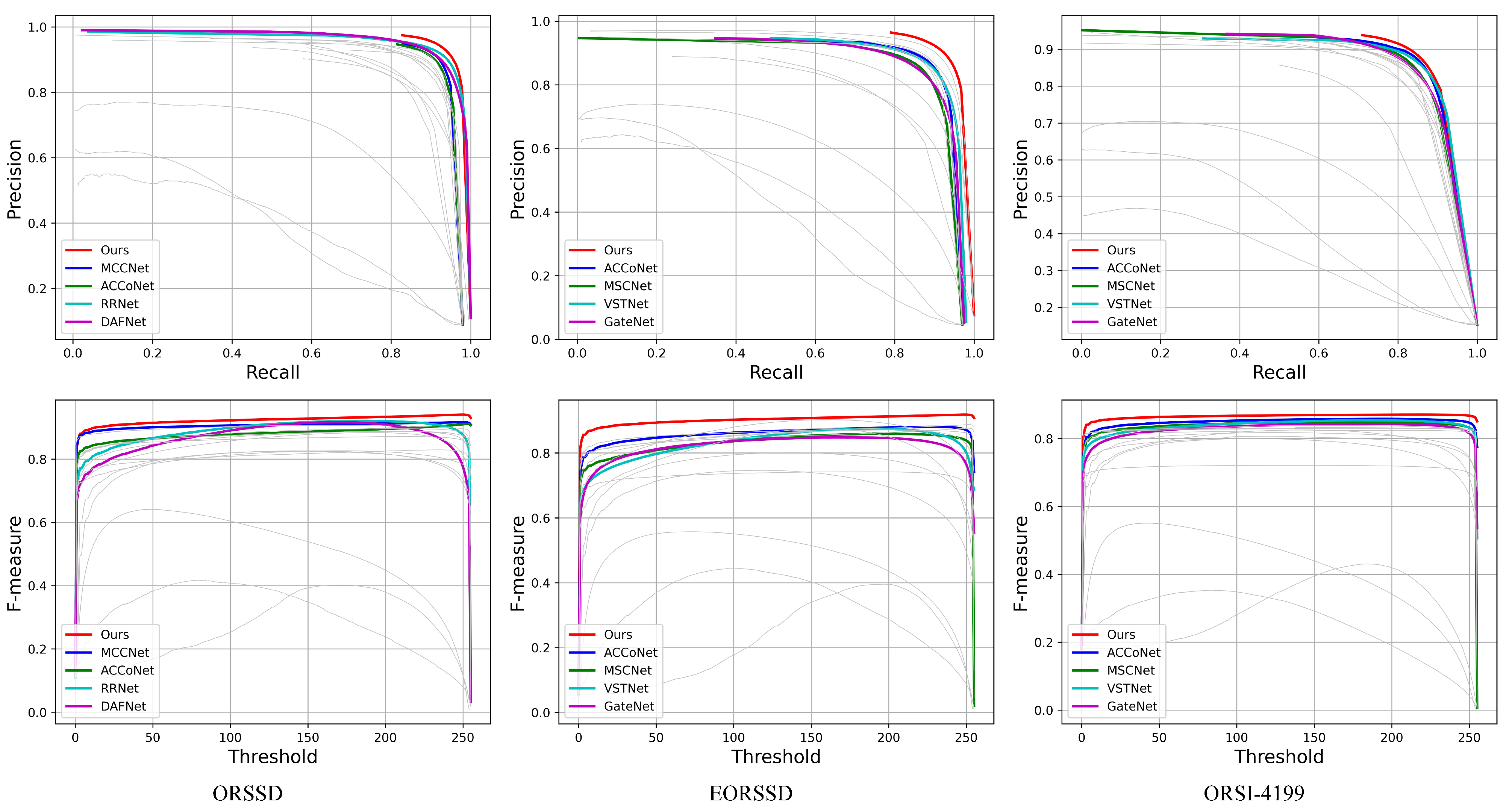
Quantitative comparison of ORSSD: We present the performance of our method TCM-Net for the ORSSD [18] dataset by quantitatively comparing it with other methods. The evaluation was conducted based on three metrics: MAE, max F-measure ($F_{\beta }^{\max }$) and S-measure ($S_m$), and the results are shown in

Table 1. Quantitative results for the three common ORSI-SOD datasets. The top three results are highlighted in red, blue and green, respectively.

Methods	ORSSD [18]			EORSSD [19]			ORSI-4199 [20]
	${\mathit{F}}_{\mathit{\beta }}^{\mathbf{max}}$↑	MAE↓	${\mathit{S}}_{\mathit{m}}$↑	${\mathit{F}}_{\mathit{\beta }}^{\mathbf{max}}$↑	MAE↓	${\mathit{S}}_{\mathit{m}}$↑	${\mathit{F}}_{\mathit{\beta }}^{\mathbf{max}}$↑	MAE↓	${\mathit{S}}_{\mathit{m}}$↑
LC (2006) [32]	0.4162	0.1243	0.5904	0.4450	0.0871	0.5926	0.3532	0.1904	0.5248
FT (2009) [33]	0.4023	0.3889	0.4269	0.3955	0.4221	0.4061	0.4303	0.4109	0.4600
MBD (2015) [58]	0.6412	0.0766	0.7018	0.5575	0.0526	0.6758	0.5508	0.1353	0.6247
CPDNet (2019) [6]	0.8259	0.0219	0.8651	0.7466	0.0201	0.8237	0.7996	0.0538	0.8245
SCRNet (2019) [8]	0.8245	0.0232	0.8558	0.8016	0.0127	0.8403	0.8176	0.0443	0.8452
PoolNet (2019) [7]	0.8293	0.0328	0.8660	0.7421	0.0191	0.8258	0.7213	0.0701	0.7664
F3Net (2020) [5]	0.8820	0.0161	0.9011	0.8764	0.0094	0.9085	0.8242	0.0414	0.8419
GateNet (2020) [9]	0.8885	0.0139	0.9133	0.8483	0.0102	0.8953	0.8429	0.0392	0.8595
VST (2021) [10]	0.8765	0.0115	0.9152	0.8749	0.0070	0.9143	0.8543	0.0306	0.8752
MJRBMNet (2021) [20]	0.8874	0.0131	0.9270	0.8709	0.0097	0.9247	0.8386	0.0384	0.8637
EMFINet (2022) [22]	0.9066	0.0125	0.9364	0.8717	0.0073	0.9279	0.8327	0.0375	0.8566
RRNet (2021) [41]	0.9210	0.0117	0.9268	0.9031	0.0082	0.9203	0.8070	0.0505	0.8317
DAFNet (2020) [19]	0.9166	0.0119	0.9154	0.8752	0.0088	0.8868	0.8252	0.0449	0.8471
LVNet (2019) [18]	0.8263	0.0207	0.8813	0.7824	0.0145	0.8650	-	-	-
ACCoNet (2022) [42]	0.9112	0.0103	0.9336	0.8818	0.0075	0.9335	0.8584	0.0328	0.8800
MSCNet (2022) [43]	0.8962	0.0120	0.9293	0.8597	0.0084	0.9180	0.8487	0.0377	0.8584
MCCNet (2021) [40]	0.9163	0.0094	0.9421	0.8875	0.0068	0.9329	0.8301	0.0379	0.8517
Ours	0.9359	0.0081	0.9428	0.9144	0.0066	0.9332	0.8717	0.0275	0.8760

. Our method demonstrates superior performance compared to all other methods on all three metrics; while MCCNet [40] is the best performer among the remaining 17 methods, our method exhibits even better performance. Specifically, our method outperforms MCCNet with a 2.14% improvement in $F_{\beta }^{\max }$, a 13.8% lower MAE and a 0.07% better $S_m$. Despite RRNet [41] and DAFNet [19] achieving higher $F_{\beta }^{\max }$ scores of 0.9210 and 0.9166, our method surpasses them by 1.62% and 2.11% in the $F_{\beta }^{\max }$ metric, respectively. Furthermore, Figure 7 illustrates the PR curve and the F-measure curve. In the three datasets with 17 methods, our model’s PR curve is positioned closer to the upper right corner, while our F-measure curve covers a larger area compared to other methods.

(b)

Quantitative comparison of EORSSD: We present a quantitative comparison of our approach with other methods on the EORSSD [19] dataset, as shown in the middle column of Table 1. Additionally, we plotted the PR curve and the F-measurement curve in Figure 7, which highlight our method’s superior performance. Among the compared methods, our approach achieves the best performance in two metrics, MAE and $F_{\beta }^{\max }$, and also has the best PR curve and F-measurement curve. However, our $S_m$ metric is slightly behind ACCoNet [42] by 0.03%. Our $S_m$ value is 0.9332, whereas ACCoNet’s $S_m$ is 0.9335. Despite this, our $F_{\beta }^{\max }$ outperforms ACCoNet by 3.70%, and our MAE is 12% lower. Notably, RRNet [41] has the highest $F_{\beta }^{\max }$ value of 0.9031 among all the compared methods, except our approach. However, our $F_{\beta }^{\max }$ is still superior to RRNet by 1.25%.

(c)

Quantitative comparison of ORSI-4199: Based on the ORSI-4199 dataset [20], we performed a quantitative comparison of the three metrics and present the results in Table 1. The corresponding PR curve and F-measure curve are shown in Figure 7 on the right. Overall, our method outperforms other methods, achieving values of 0.0275, 0.8717 and 0.8760, respectively. In addition, our method showed the best performance in the PR curve F-measure curve. Among the other methods, ACCoNet [42] achieved the best results with MAE, $F_{\beta }^{\max }$ and $S_m$ values of 0.0328, 0.8584 and 0.8800, respectively. Compared to ACCoNet, our $S_m$ was 0.46% lower, but our $F_{\beta }^{\max }$ was 1.55% higher and MAE was 19.3% lower. Moreover, our comparison with VSTNet [10], which showed the highest performance among the NSI-SOD methods, demonstrated the high applicability of the transformer model in the SOD task. VSTNet achieved values of 0.8543, 0.0306 and 0.8752 for MAE, $F_{\beta }^{\max }$ and $S_m$, respectively. Our method achieved a better $F_{\beta }^{\max }$ (improved by 2.04%), lower MAE (reduced by 11.3%) and slightly improved $S_m$ (by 0.09%) compared to VSTNet.

Our quantitative comparison results demonstrate that our proposed method outperforms 17 other methods for ORSI-SOD. We provide a new state-of-the-art benchmark for comparison. The success of our model is attributed to the proposed dual-path complementary codec network structure and gating mechanism, which is better suited for ORSIs. We conducted more detailed ablation experiments to further investigate the advantages of each module.

(2)

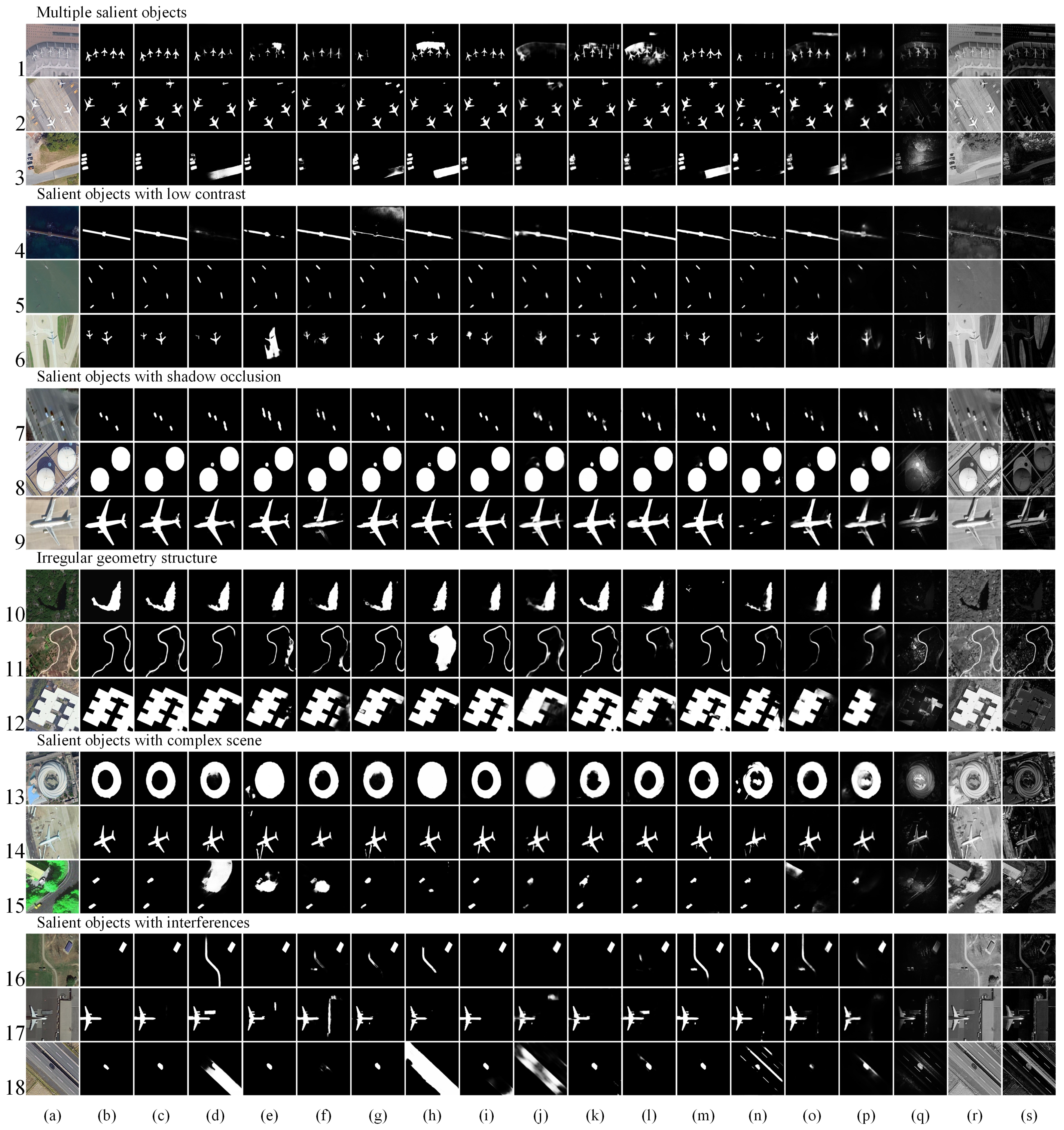
Visual comparison: To qualitatively compare all methods, we selected experimental results from the ORSI-4199 dataset, which includes representative and challenging scenes, as shown in Figure 8. These scenes involve multiple objects, complex scenes, low contrast, shadow occlusion and more. Our model’s predictions demonstrate greater completeness and accuracy in detecting salient objects compared to other methods shown in Figure 8. The specific advantages are reflected in the following aspects.

(a)

Superiority in scenes with multiple or multiscale objects: In the first and third examples of Figure 8, both traditional models (e.g., LC [32] and MBD [58] shown in Figure 8q,s) and deep-learning-based models (e.g., EMFINet [22], DAFNet [19] and F3Net [5] presented in Figure 8h,j,m) fail to highlight the foreground regions accurately, resulting in prominent errors. In contrast, our model provides complete and accurate inference for salient objects. Similarly, in the eighth and thirteenth examples of Figure 8, some state-of-the-art deep-learning models (e.g., ACCoNet [42], MCCNet [40] and MSCNet [43] depicted in Figure 8d,e,g) either incorrectly detect multiple objects or fail to fully pop out the salient objects. In stark contrast, the model shown in Figure 8 can still successfully highlight the salient objects, and our results exhibit clear boundaries, particularly in preserving the overall integrity of multiple small airplanes and a single large building. This is clearly attributed to the superiority of our U-shaped encoder–decoder architecture and the control of redundant information by the AG module.

(b)

Superiority in cluttered background and low contrast scenes: In the fourth, fifth and sixth examples of Figure 8, traditional models (e.g., LC [32] and FT [33] shown in Figure 8r,s) completely fail to detect salient objects, while deep-learning-based models (e.g., ACCoNet [42], MSCNet [43], PoolNet [7] presented in Figure 8d,g,n) either provide incomplete detection or incorrectly highlight background regions. In contrast, our model successfully detects salient bridges, four ships and two airplanes from the aforementioned three examples. Similarly, in Figure 8, for the fourteenth, fifteenth and seventeenth examples, state-of-the-art deep-learning models (e.g., ACCoNet [42], MCCNet [40] and RRNet [41]) either erroneously highlight background regions or fail to clearly distinguish salient objects, as shown in Figure 8d–f). In contrast, the model depicted in Figure 8c can fully and clearly pop out all salient objects. This is clearly attributed to our effective control of global contextual and local detailed information, as well as the LGFF module’s ability to fuse information from both sources effectively.

(c)

Superiority in salient regions with complicated edges or irregular topology: In the tenth, eleventh and twelfth examples of Figure 8, both traditional models (e.g., LC [32] and MBD [58] shown in Figure 8q,s) and deep-learning-based models (e.g., ACCoNet [42], MCCNet [40], EMFINet [22], MJRBMNet [20] and GateNet [9]) presented in Figure 8d,e,h,i,l fail to accurately delineate the lake regions comprehensively and also fall short in detecting irregular rivers and buildings. In contrast, our model, as shown in Figure 8c, outperforms the other models. The forest regions are effectively suppressed, irregular lakes are fully highlighted and, for irregular topological structures of rivers and buildings, our model is capable of generating a more complete saliency map with more accurate boundaries. It is evident that these superior results are attributed to the addition of edge supervision in our hybrid loss and our effective control of global-to-local information for image localization.

(3)

Attribute-based study: In the latest ORSI-4199 dataset [20], each image is meticulously categorized according to the distinctive attributes commonly found in ORSIs. These attributes include the presence of big salient objects (BSOs), small salient objects (SSOs), off center (OC) objects, complex salient objects (CSOs), complex scenes (CSs), narrow salient objects (NSOs), multiple salient objects (MSOs), low contrast scenes (LCSs) and incomplete salient objects (ISOs). These annotations allow us to compare the strengths and weaknesses of our proposed model and other models under different conditions.

Table 2. Results of attribute-based tests on the ORSI-4199 [20] dataset. We show the max F-measure scores for a total of 14 methods, including ours. The last row shows the average performance. These top three scores are highlighted in red, blue and green, respectively.

Attr	BSO	CS	CSO	ISO	LSO	MSO	NSO	OC	SSO	Avg
ACCoNet [42]	0.9207	0.8976	0.8864	0.9012	0.7713	0.8486	0.8751	0.8329	0.7843	0.8576
DAFNet [19]	0.8875	0.8682	0.8631	0.8598	0.7444	0.8048	0.8458	0.7808	0.7370	0.8213
EMFINet [22]	0.9185	0.8790	0.8870	0.9018	0.7418	0.8188	0.8432	0.7562	0.7286	0.8305
RRNet [41]	0.8533	0.8413	0.8359	0.8314	0.7354	0.8017	0.8393	0.7697	0.7237	0.8035
MJRBNet [20]	0.8951	0.8800	0.8601	0.8835	0.7468	0.8415	0.8471	0.8282	0.7724	0.8394
MCCNet [40]	0.9056	0.8749	0.8685	0.8858	0.7383	0.8075	0.8477	0.8060	0.7414	0.8306
MSCNet [43]	0.9014	0.8886	0.8676	0.8961	0.7659	0.8375	0.8811	0.8123	0.7699	0.8467
VSTNet [10]	0.9107	0.8978	0.9071	0.9269	0.7743	0.8299	0.9022	0.8103	0.7435	0.8559
F3Net [5]	0.8852	0.8625	0.8578	0.8796	0.7495	0.8249	0.8668	0.7861	0.7426	0.8283
PoolNet [7]	0.7473	0.7436	0.7365	0.7096	0.6442	0.7464	0.7669	0.6962	0.6605	0.7168
GateNet [9]	0.9140	0.8841	0.8807	0.8954	0.7598	0.8372	0.8535	0.8059	0.7624	0.8437
SCRNNet [8]	0.8945	0.8647	0.8658	0.8752	0.7283	0.8181	0.8296	0.7875	0.7354	0.8221
CPDNet [6]	0.8850	0.8479	0.8482	0.8631	0.7176	0.7839	0.8009	0.7740	0.7070	0.8031
Ours	0.9324	0.9142	0.9037	0.9275	0.7845	0.8515	0.8987	0.8386	0.7920	0.8715

shows the $F_{\beta }^{\max }$ values of our model and other state-of-the-art models. Our model ranks first in seven of the nine attributes and second in scores for the remaining two attributes. Additionally, we used radar plots for the first time to depict the $F_{\beta }^{\max }$ values of the top five ranked methods for different attributes, and the results confirm that our model outperforms existing models in the majority of challenging scenarios, as shown in Figure 9.

4.4. Extension Experiment on NSI Datasets

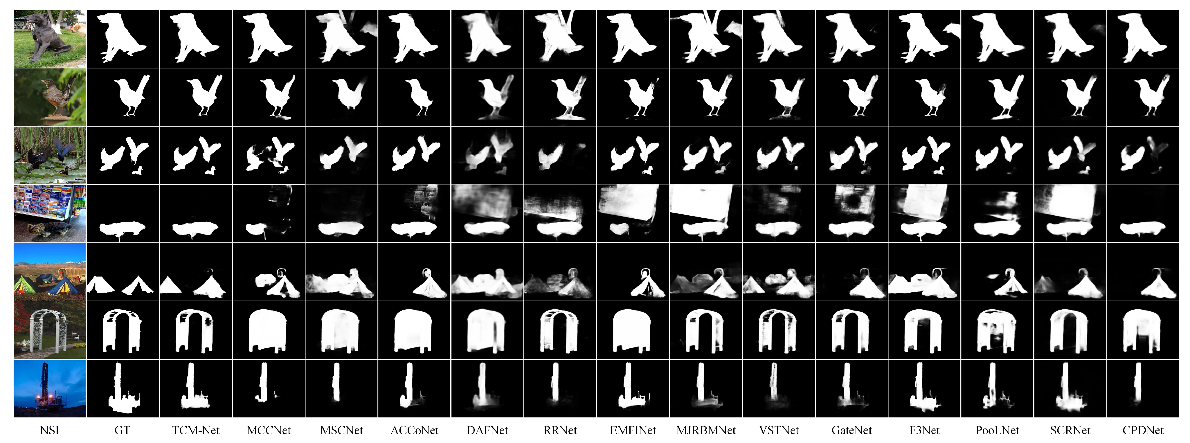
To further investigate the compatibility and scalability of TCM-Net, we performed a comparison with 13 state-of-the-art deep-learning-based SOD models, namely VST [10], GateNet [9], F3Net [5], PoolNet [7], SCRNet [8], CPDNet [6], MCCNet [40], MSCNet [43], ACCoNet [42], DAFNet [19], EMFINet [22], MJRBMNet [20] and RRNet [41], on three public NSI-SOD datasets. From the three evaluation metrics in

Table 3. Quantitative results for the three public NSI-SOD datasets. The top three results are highlighted in red, blue and green, respectively.

Methods	DUT-OMRON [59]			DUTS-TE [60]			HKU-IS [61]
	${\mathit{F}}_{\mathit{\beta }}^{\mathbf{max}}$↑	MAE↓	${\mathit{S}}_{\mathit{m}}$↑	${\mathit{F}}_{\mathit{\beta }}^{\mathbf{max}}$↑	MAE↓	${\mathit{S}}_{\mathit{m}}$↑	${\mathit{F}}_{\mathit{\beta }}^{\mathbf{max}}$↑	MAE↓	${\mathit{S}}_{\mathit{m}}$↑
CPDNet [6]	0.7513	0.0550	0.8237	0.8374	0.0434	0.8675	0.9115	0.0336	0.9078
SCRNet [8]	0.7628	0.0626	0.8300	0.8556	0.0440	0.8791	0.9220	0.0343	0.9166
PoolNet [7]	0.7280	0.0597	0.8049	0.8187	0.0457	0.8529	0.8911	0.0386	0.8912
F3Net [5]	0.7777	0.0578	0.8346	0.8714	0.0373	0.8874	0.9287	0.0279	0.9205
GateNet [9]	0.7748	0.0535	0.8370	0.8723	0.0370	0.8895	0.9239	0.0323	0.9188
VST [10]	0.8066	0.0549	0.8562	0.8780	0.0370	0.8966	0.9371	0.0296	0.9288
MJRBMNet [20]	0.7493	0.0663	0.8192	0.8267	0.0521	0.8607	0.9071	0.0376	0.9066
EMFINet [22]	0.7697	0.0598	0.8281	0.8278	0.0500	0.8585	0.9138	0.0336	0.9066
RRNet [41]	0.7728	0.0622	0.8326	0.7830	0.0621	0.8279	0.8671	0.0523	0.8717
DAFNet [19]	0.7268	0.0778	0.8004	0.7523	0.0770	0.8084	0.8616	0.0622	0.8674
ACCoNet [42]	0.7635	0.0631	0.8253	0.8282	0.0500	0.8588	0.9128	0.0340	0.9062
MSCNet [43]	0.7711	0.0632	0.8254	0.8188	0.0537	0.8492	0.9014	0.0415	0.8940
MCCNet [40]	0.7750	0.0576	0.8296	0.8356	0.0465	0.8616	0.9167	0.0326	0.9054
Ours	0.7973	0.0535	0.8426	0.8839	0.0336	0.8953	0.9378	0.0243	0.9283

, it can be seen that our model outperforms most of the deep-learning-based models for the NSI dataset. Additionally, Figure 10 shows some visual contrast results in NSI, where the salient object localization detected by our method is more accurate and has more details. This is primarily attributed to TCM-Net’s ability to learn both global and local features.

4.5. Ablation Study

(1)

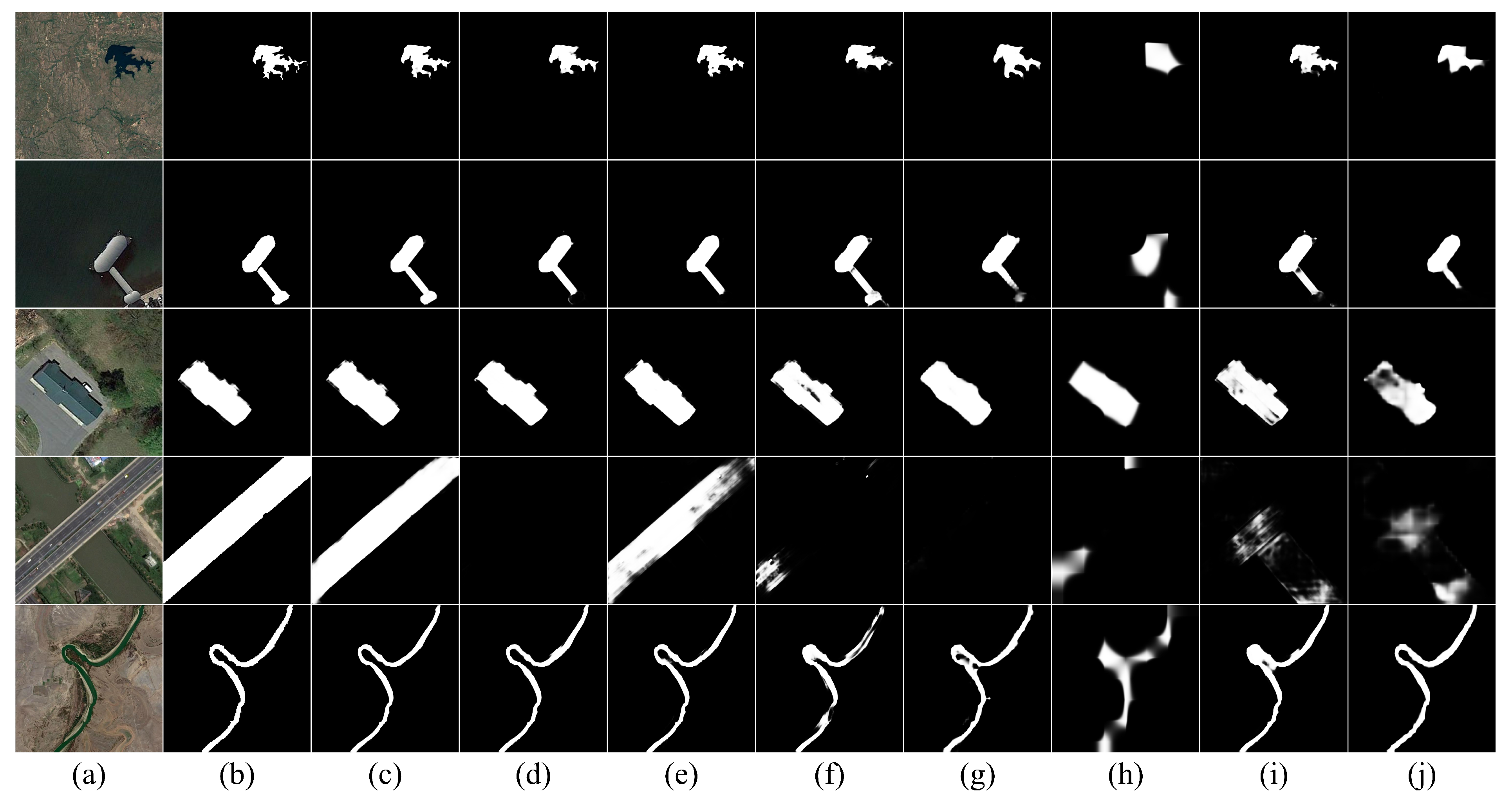
Module ablation experiments: We conducted module ablation experiments on the EORSSD dataset to evaluate the effectiveness of our proposed ResNet34+Swin transformer model compared to baseline models using either ResNet34 or the Swin transformer alone. Additionally, we evaluated the U-shaped encoder–decoder network architecture to determine its effectiveness, with the modular ablation study focusing on two specific modules, namely LGFF and AG. To visually demonstrate the effectiveness of our proposed architecture and modules, we present saliency maps in Figure 11, highlighting the impact of different ablation modules and baselines.

As shown in Figure 11d,e, the incorporation of AG modules significantly improves the ability to characterize feature information across multiple layers. This results in the reduction in redundant interference information and the suppression of image noise, which ultimately leads to improved prediction accuracy. Our LGFF module successfully integrates global and local information, as shown in Figure 11d,f, effectively capturing both macro global context and fine local details. While the direct U-shaped network structure, as shown in the second and fourth panels of Figure 11, may have slightly lower accuracy, it outperforms in SOD with irregular topology, as shown in the first and fifth panels of Figure 11. Comparing panels (g)-(h), (i)-(j) in Figure 11, it can be seen that the use of the U-shaped codec structure yields significantly better results than relying solely on the basic models of the Swin transformer and ResNet34. This approach provides better detection results and captures more detail information.

Table 4. Quantitative evaluation of ablation studies on the EORSSD dataset. “U” is the u-shaped codec structure.

Backbone	LGFF	AG	${\mathit{F}}_{\mathit{\beta }}^{\mathbf{max}}$↑	MAE↓	${\mathit{S}}_{\mathit{m}}$↑
Swin transformer			0.5409	0.0214	0.7433
Swin + U			0.8654	0.083	0.8998
ResNet34			0.7981	0.0151	0.8669
ResNet34 + U			0.8563	0.0124	0.8990
Baseline			0.8980	0.0077	0.9235
Baseline	✓		0.9029	0.0075	0.9246
Baseline		✓	0.9126	0.0067	0.9318
Baseline	✓	✓	0.9144	0.0066	0.9332

shows the quantitative results for the variables in our study. We performed eight ablation experiments to evaluate the effectiveness of the U-shape codec architecture, the LGFF module and the AG module. We included the baseline codec layer (ResNet34 + Swin transformer + U-shape codec architecture) in the appropriate position to meet the requirements of the ablation experiments, which included the LGFF module as a variable. Although the performance of the TCM-Net baseline was lower than many of the comparison methods in Table 1, it can still be considered a relatively good model. To solve the multi-scale problem of ORSI, we utilized a U-shape codec architecture to improve the detection accuracy. This was achieved by feeding the features of the coding part into the decoding module through skip connections. The results in Table 4 show a significant performance improvement with the adoption of the U-shape codec architecture. Adding the U-shape architecture to ResNet34 improves the $F_{\beta }^{\max }$ by 7.3%, the $S_m$ by 3.7% and reduces the MAE by 17.9% compared to the original ResNet34. In addition, adding the U-shape architecture to the Swin transformer results in even more significant improvements. The $F_{\beta }^{\max }$ is improved by 60%, the $S_m$ is improved by 21.1%, and the MAE is reduced by 61.2% compared to the original Swin transformer.

To optimize the fusion of local and global information from the CNN and transformer, we introduced the LGFF module. However, the improvement achieved with the LGFF module is not significant because our TCM-Net baseline is a 7-layer decoding structure, and adding the LGFF module results in a reduction of one decoding layer. To improve feature extraction and reduce redundant information, our AG module shows a significant performance improvement, as evidenced by the improvement in $S_m$ from 0.8980 to 0.9126, $S_m$ from 0.9235 to 0.9332 and the reduction in MAE from 0.77 to 0.66. Our TCM-Net structure integrates the local and global information using the LGFF module and the U-shaped architecture for the decoder, while the AG module controls the redundant information to improve feature characterization. Compared to our network baseline, the TCM-Net structure achieves a 1.83% improvement in $F_{\beta }^{\max }$, 1.05% improvement in $S_m$ and 14.5% reduction in MAE.

(2)

Loss ablation experiments: We performed ablation experiments on the EORSSD dataset [19] to demonstrate the effectiveness of our hybrid loss function strategy, which is specifically designed for the network structure. To demonstrate the complementarity of BCE, IoU, SSIM and Fm in the loss function, we evaluated our loss function using four common loss function strategies: (1) training our model only with BCE loss, e.g., [6]; (2) training our model with BCE-IoU loss, e.g., [42]; (3) training our model jointly with the three loss functions of BCE, IoU and SSIM, e.g., [22]; (4) training our model jointly with the three loss functions of BCE, IoU and Fm, e.g., [40]; and (5) using our selected hybrid function and allocation strategy that includes BCE, IoU, SSIM and Fm. The results are shown in

Table 5. Quantitative evaluation of loss function ablation studies on the EORSSD dataset.

No.	BCE	IoU	SSIM	Fm	${\mathit{F}}_{\mathit{\beta }}^{\mathbf{max}}$↑	MAE↓	${\mathit{S}}_{\mathit{m}}$↑
1	✓				0.8459	0.0095	0.8864
2	✓	✓			0.9119	0.0070	0.9309
3	✓	✓	✓		0.9080	0.0069	0.9295
4	✓	✓		✓	0.9103	0.0071	0.9314
5	✓	✓	✓	✓	0.9038	0.0071	0.9272
6 (Ours)	✓	✓	✓	✓	0.9144	0.0066	0.9332

.

In this study, we evaluated the effectiveness of different loss functions for our deep-learning-based ORSI-SOD model on the EORSSD dataset. Our model using only the BCE loss function was the least effective, achieving $F_{\beta }^{\max }$ of 0.8459, MAE of 0.0095 and $S_m$ of 0.8864. Nevertheless, our model outperformed four out of the six deep-learning-based ORSI-SODs listed in Table 1. In Experiment 2, we used the common loss strategy BCE-IOU loss and achieved better performance than the 17 state-of-the-art methods in Table 1, with $F_{\beta }^{\max }$ of 0.9129, MAE of 0.0070 and $S_m$ of 0.9309. This result indirectly proves that our model is more suitable for combining multiple loss functions.

We also tested our model using BCE-IOU loss in combination with the SSIM loss function and the Fm loss function, respectively. Compared to BCE-IOU loss, the hybrid loss function using SSIM resulted in a decrease in $F_{\beta }^{\max }$ and $S_m$ to 0.9080 and 0.9295, respectively, with only a small decrease in MAE to 0.0069. The hybrid loss function using Fm loss resulted in a decrease in $F_{\beta }^{\max }$ to 0.9103, an increase in MAE to 0.0071 and an improvement in $S_m$ to 0.9314. We also compared our designed hybrid loss function strategy with a control group that stacked detail loss, global loss and final prediction loss together. The results showed that our designed strategy outperformed the control group, with $F_{\beta }^{\max }$ of 0.9144, MAE of 0.0066 and $S_m$ of 0.9332, while the control group achieved $F_{\beta }^{\max }$ of 0.9038, MAE of 0.0071 and $S_m$ of 0.9272. These results show that simply stacking other loss functions does not necessarily improve the performance of the network. Our experimental comparison confirms that the best performance is achieved using our hybrid loss function strategy, which is specifically designed for the network structure.

4.6. Cross-Validation Analysis of the Model

It is crucial to ensure that the model does not suffer from overfitting or underfitting. Ten-fold cross-validation is a common approach to evaluate model overfitting. We performed a 10-fold cross-validation experiment on the EORSSD dataset to check for overfitting. The results in

Table 6. Results of the 10-fold cross-validation of the model on the EORSSD dataset.

NO.	1	2	3	4	5	6	7	8	9	10	Avg
$F_{\beta }^{\max }$	0.9317	0.9230	0.9259	0.9295	0.9310	0.9299	0.9201	0.8811	0.9033	0.9149	0.9190
MAE	0.0079	0.0070	0.0064	0.0086	0.0059	0.0066	0.0068	0.0104	0.0078	0.0139	0.0081
$S_m$	0.9372	0.9344	0.9403	0.9353	0.9468	0.9371	0.9363	0.9125	0.9312	0.9341	0.9345

demonstrate that our model performs well on each experiment of the dataset without overfitting, indicating the robustness of the proposed model.

4.7. Evaluation of Loss Weighting

The weighting of different loss functions could affect detection performance. To investigate the impact of the weight of loss function on performance, we adjusted the weight values from 0.1 to 1 in the comparison experiments. As can be seen from

Table 7. Results for different weights of the loss function on the EORSSD dataset.

Weight	0.1	0.2	0.3	0.4	0.5	0.6	0.7	0.8	0.9	1
$F_{\beta }^{\max }$	0.9051	0.9144	0.9089	0.9007	0.8819	0.9018	0.9029	0.9011	0.8951	0.9061
MAE	0.0075	0.0066	0.0072	0.0074	0.0108	0.0078	0.0076	0.0080	0.0076	0.0075
$S_m$	0.9248	0.9332	0.9297	0.9212	0.9121	0.9237	0.9241	0.9231	0.9200	0.9258

, the optimal performance can be achieved by setting the weight to 0.2.

4.8. Complexity Analysis

We have conducted a comparison between multiple deep-learning-based algorithms for SOD, evaluating their complexities in regard to model parameters (#Param), floating-point operations (FLOPs) and test frames per second (FPS). Please refer to

Table 8. Comparison of model complexity of deep-learning-based methods.

Complexity	CPD	SCRN	Pool	F3Net	Gate	VST	EMFI	RRNet	DAF	ACCo	MSC	MCC	TCM
	[6]	[8]	[7]	[5]	[9]	[10]	[22]	[41]	[19]	[42]	[43]	[40]	Ours
#Param (M)	47	25	68	25	128	44	95	83	29	127	3	68	89
FLOPs (G)	17	15	51	16	162	23	177	138	68	51	5	117	102
FPS (s)	11	12	11	20	10	11	6	12	14	11	11	13	12

for details. The number of #Param is measured in millions (M), FLOPs is measured in giga (G) and FPS is measured in seconds (s). In the case of TCM-Net, FLOPs were tested using input images with a resolution of 1024 × 1024. Despite our model having an above average number of #Param and FLOP values, our FPS value are still within the range of mainstream levels.

4.9. Failure Case

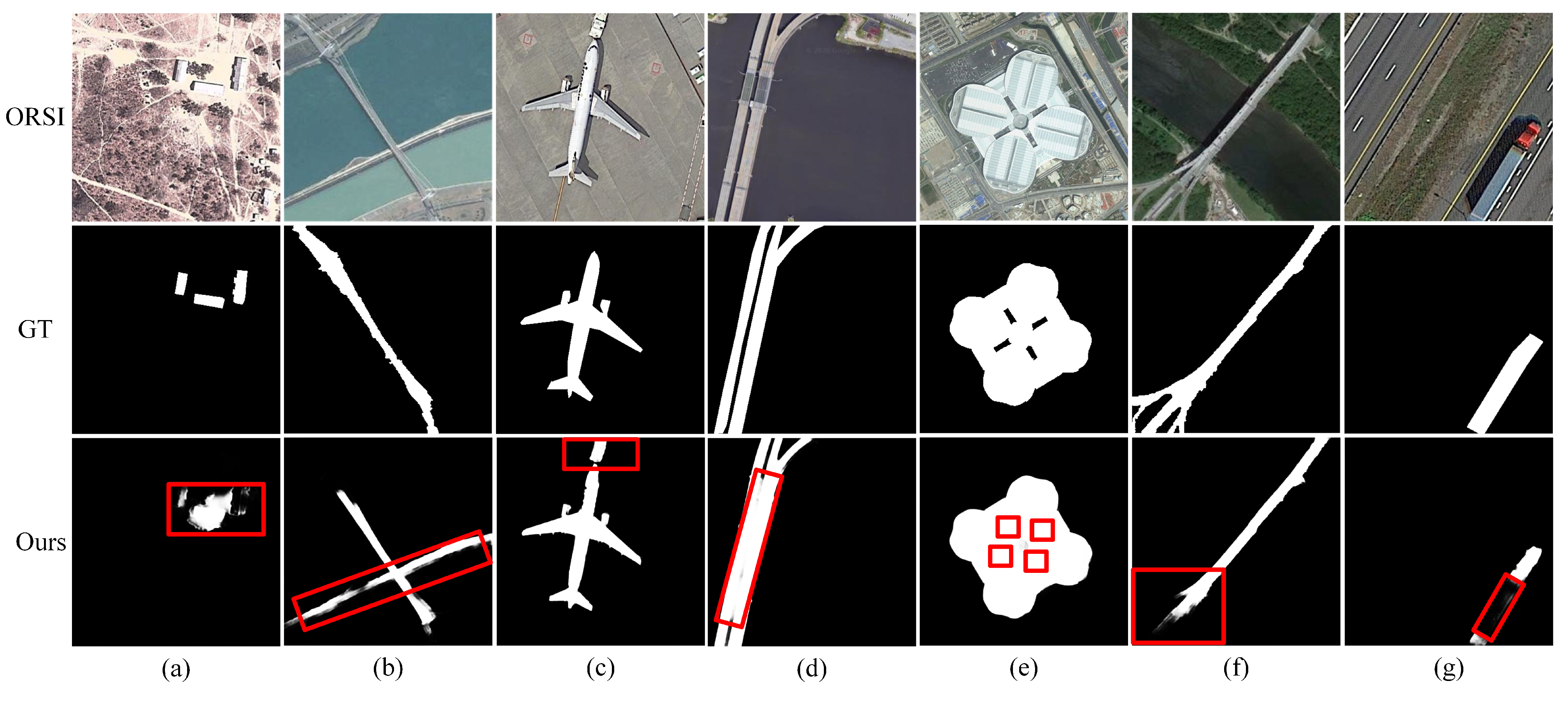
Although TCM-Net shows superior performance on three public ORSI-SOD datasets. For some very challenging examples, our method still cannot achieve perfect results.

The model exhibits poor performance in highly cluttered backgrounds and low contrast scenes, as shown in Figure 12a, making it difficult to clearly segment objects. Additionally, the subtle difference between salient objects and non-salient objects causes our model to misclassify non-salient objects as the foreground, presented in Figure 12b,c. Furthermore, our model misidentifies portions between adjacent salient objects and background regions, depicted in Figure 12d,e. Finally, for salient object portions that are similar to the background, our model may miss them and treat them as background regions during detection, as illustrated in Figure 12f,g. The aforementioned concerns could necessitate additional model optimization and data acquisition from diverse scenarios to augment model training.

5. Conclusions

This article propose a novel ORSI-SOD methodology called TCM-Net, which ingeniously combines the ability of local feature extraction of a CNN with the global modeling of a transformer. An LGFF module was designed to integrate local and global feature information into corresponding decoding layers. To address the multiscale problem of ORSIs, a U-shaped network structure is employed. An AG module was also designed to filter feature information in layers, reduce redundancy, suppress noise and emphasize spatial and channel features. To ensure precision of the final detection map and to address the problem of edge blur in ORSIs, edge information is included in the hybrid supervision function. However, high-resolution input images increase the computational cost of the model, while increasing accuracy results in decreased speed. Future research will focus on lightweight model design.

In our method, instances of detection failures still persist, primarily attributable to the limited scale of the training dataset in ORSI-SOD. In our forthcoming research endeavors, we plan to address this issue using large-scale models, such as SAM [62], commonly employed in segmentation tasks. We plan to adapt these models to downstream tasks through fine-tuning or prompt-tuning paradigms, thereby capitalizing on the rich knowledge embedded within these expansive models to mitigate the challenges posed by data scarcity.

References

1. Zeng, Y.; Zhuge, Y.; Lu, H.; Zhang, L. Joint learning of saliency detection and weakly supervised semantic segmentation. In Proceedings of the IEEE/CVF International Conference on Computer Vision, Seoul, Republic of Korea, 27 October–2 November 2019; pp. 7223–7233. [Google Scholar]
2. Fang, Y.; Lin, W.; Chen, Z.; Tsai, C.M.; Lin, C.W. A video saliency detection model in compressed domain. IEEE Trans. Circuits Syst. Video Technol. 2013, 24, 27–38. [Google Scholar] [CrossRef]
3. Yuan, Y.; Lu, Y.; Wang, Q. Tracking as a whole: Multi-target tracking by modeling group behavior with sequential detection. IEEE Trans. Intell. Transp. Syst. 2017, 18, 3339–3349. [Google Scholar] [CrossRef]
4. Yang, S.; Jiang, Q.; Lin, W.; Wang, Y. SGDNet: An End-to-End Saliency-Guided Deep Neural Network for No-Reference Image Quality Assessment. In Proceedings of the 27th ACM International Conference on Multimedia, MM 2019, Nice, France, 21–25 October 2019; Amsaleg, L., Huet, B., Larson, M.A., Gravier, G., Hung, H., Ngo, C., Ooi, W.T., Eds.; ACM: New York, NY, USA, 2019; pp. 1383–1391. [Google Scholar] [CrossRef]
5. Wei, J.; Wang, S.; Huang, Q. F3Net: Fusion, feedback and focus for salient object detection. Proc. AAAI Conf. Artif. Intell. 2020, 34, 12321–12328. [Google Scholar] [CrossRef]
6. Wu, Z.; Su, L.; Huang, Q. Cascaded partial decoder for fast and accurate salient object detection. In Proceedings of the IEEE/CVF Conference on Computer Vision and Pattern Recognition, Long Beach, CA, USA, 16–20 June 2019; pp. 3907–3916. [Google Scholar]
7. Liu, J.J.; Hou, Q.; Cheng, M.M.; Feng, J.; Jiang, J. A simple pooling-based design for real-time salient object detection. In Proceedings of the IEEE/CVF Conference on Computer Vision and Pattern Recognition, Long Beach, CA, USA, 16–20 June 2019; pp. 3917–3926. [Google Scholar]
8. Wu, Z.; Su, L.; Huang, Q. Stacked cross refinement network for edge-aware salient object detection. In Proceedings of the IEEE/CVF International Conference on Computer Vision, Seoul, Republic of Korea, 27 October–2 November 2019; pp. 7264–7273. [Google Scholar]
9. Zhao, X.; Pang, Y.; Zhang, L.; Lu, H.; Zhang, L. Suppress and balance: A simple gated network for salient object detection. In Proceedings of the Computer Vision–ECCV 2020: 16th European Conference, Glasgow, UK, 23–28 August 2020; Proceedings, Part II 16. Springer: Berlin/Heidelberg, Germany, 2020; pp. 35–51. [Google Scholar]
10. Liu, N.; Zhang, N.; Wan, K.; Shao, L.; Han, J. Visual saliency transformer. In Proceedings of the IEEE/CVF International Conference on Computer Vision, Virtual, 11–17 October 2021; pp. 4722–4732. [Google Scholar]
11. Xie, C.; Xia, C.; Ma, M.; Zhao, Z.; Chen, X.; Li, J. Pyramid grafting network for one-stage high resolution saliency detection. In Proceedings of the IEEE/CVF Conference on Computer Vision and Pattern Recognition, New Orleans, LA, USA, 19–24 June 2022; pp. 11717–11726. [Google Scholar]
12. Qin, X.; Zhang, Z.; Huang, C.; Gao, C.; Dehghan, M.; Jagersand, M. Basnet: Boundary-aware salient object detection. In Proceedings of the IEEE/CVF Conference on Computer Vision and Pattern Recognition, Long Beach, CA, USA, 16–20 June 2019; pp. 7479–7489. [Google Scholar]
13. Qin, X.; Zhang, Z.; Huang, C.; Dehghan, M.; Zaiane, O.R.; Jagersand, M. U2-Net: Going deeper with nested U-structure for salient object detection. Pattern Recognit. 2020, 106, 107404. [Google Scholar] [CrossRef]
14. Liu, N.; Han, J.; Yang, M.H. Picanet: Learning pixel-wise contextual attention for saliency detection. In Proceedings of the IEEE Conference on Computer Vision and Pattern Recognition, Salt Lake CIty, UT, USA, 18–22 June 2018; pp. 3089–3098. [Google Scholar]
15. Hou, Q.; Cheng, M.M.; Hu, X.; Borji, A.; Tu, Z.; Torr, P.H. Deeply supervised salient object detection with short connections. In Proceedings of the IEEE Conference on Computer Vision and Pattern Recognition, Honolulu, HI, USA, 21–26 July 2017; pp. 3203–3212. [Google Scholar]
16. Zhao, C. Advances of research and application in remote sensing for agriculture. Nongye Jixie Xuebao Trans. Chin. Soc. Agric. Mach. 2014, 45, 277–293. [Google Scholar]
17. Bello, O.M.; Aina, Y.A. Satellite remote sensing as a tool in disaster management and sustainable development: Towards a synergistic approach. Procedia Soc. Behav. Sci. 2014, 120, 365–373. [Google Scholar] [CrossRef]
18. Li, C.; Cong, R.; Hou, J.; Zhang, S.; Qian, Y.; Kwong, S. Nested network with two-stream pyramid for salient object detection in optical remote sensing images. IEEE Trans. Geosci. Remote Sens. 2019, 57, 9156–9166. [Google Scholar] [CrossRef]
19. Zhang, Q.; Cong, R.; Li, C.; Cheng, M.M.; Fang, Y.; Cao, X.; Zhao, Y.; Kwong, S. Dense attention fluid network for salient object detection in optical remote sensing images. IEEE Trans. Image Process. 2020, 30, 1305–1317. [Google Scholar] [CrossRef]
20. Tu, Z.; Wang, C.; Li, C.; Fan, M.; Zhao, H.; Luo, B. ORSI salient object detection via multiscale joint region and boundary model. IEEE Trans. Geosci. Remote Sens. 2021, 60, 5607913. [Google Scholar] [CrossRef]
21. Zhao, H.; Shi, J.; Qi, X.; Wang, X.; Jia, J. Pyramid scene parsing network. In Proceedings of the IEEE Conference on Computer Vision and Pattern Recognition, Honolulu, HI, USA, 21–26 July 2017; pp. 2881–2890. [Google Scholar]
22. Zhou, X.; Shen, K.; Liu, Z.; Gong, C.; Zhang, J.; Yan, C. Edge-Aware Multiscale Feature Integration Network for Salient Object Detection in Optical Remote Sensing Images. IEEE Trans. Geosci. Remote Sens. 2022, 60, 5605315. [Google Scholar] [CrossRef]
23. Chen, L.C.; Papandreou, G.; Kokkinos, I.; Murphy, K.; Yuille, A.L. Deeplab: Semantic image segmentation with deep convolutional nets, atrous convolution, and fully connected crfs. IEEE Trans. Pattern Anal. Mach. Intell. 2017, 40, 834–848. [Google Scholar] [CrossRef] [PubMed]
24. Vaswani, A.; Shazeer, N.; Parmar, N.; Uszkoreit, J.; Jones, L.; Gomez, A.N.; Kaiser, Ł.; Polosukhin, I. Attention is all you need. Adv. Neural Inf. Process. Syst. 2017, 30, 5998–6008. [Google Scholar]
25. Chen, K.; Zou, Z.; Shi, Z. Building Extraction from Remote Sensing Images with Sparse Token Transformers. Remote. Sens. 2021, 13, 4441. [Google Scholar] [CrossRef]
26. Fang, J.; Lin, H.; Chen, X.; Zeng, K. A Hybrid Network of CNN and Transformer for Lightweight Image Super-Resolution. In Proceedings of the IEEE/CVF Conference on Computer Vision and Pattern Recognition Workshops, CVPR Workshops 2022, New Orleans, LA, USA, 19–20 June 2022; pp. 1102–1111. [Google Scholar] [CrossRef]
27. Borji, A.; Cheng, M.M.; Jiang, H.; Li, J. Salient object detection: A benchmark. IEEE Trans. Image Process. 2015, 24, 5706–5722. [Google Scholar] [CrossRef]
28. Itti, L.; Koch, C.; Niebur, E. A model of saliency-based visual attention for rapid scene analysis. IEEE Trans. Pattern Anal. Mach. Intell. 1998, 20, 1254–1259. [Google Scholar] [CrossRef]
29. Klein, D.A.; Frintrop, S. Center-surround divergence of feature statistics for salient object detection. In Proceedings of the 2011 International Conference on Computer Vision, Virtual, 11–17 October 2021; pp. 2214–2219. [Google Scholar]
30. Liu, Z.; Zou, W.; Le Meur, O. Saliency tree: A novel saliency detection framework. IEEE Trans. Image Process. 2014, 23, 1937–1952. [Google Scholar]
31. Zhu, W.; Liang, S.; Wei, Y.; Sun, J. Saliency optimization from robust background detection. In Proceedings of the IEEE Conference on Computer Vision and Pattern Recognition, Columbus, OH, USA, 23–28 June 2014; pp. 2814–2821. [Google Scholar]
32. Zhai, Y.; Shah, M. Visual attention detection in video sequences using spatiotemporal cues. In Proceedings of the 14th ACM International Conference on MULTIMEDIA, Santa Barbara, CA, USA, 23–27 October 2006; pp. 815–824. [Google Scholar]
33. Achanta, R.; Hemami, S.; Estrada, F.; Susstrunk, S. Frequency-tuned salient region detection. In Proceedings of the 2009 IEEE Conference on Computer Vision and Pattern Recognition, Miami, FL, USA, 20–25 June 2009; pp. 1597–1604. [Google Scholar]
34. Zhou, L.; Yang, Z.; Yuan, Q.; Zhou, Z.; Hu, D. Salient region detection via integrating diffusion-based compactness and local contrast. IEEE Trans. Image Process. 2015, 24, 3308–3320. [Google Scholar] [CrossRef]
35. Liu, T.; Sun, J.; Zheng, N.N.; Tang, X.; Shum, H.Y. Learning to Detect A Salient Object. In Proceedings of the 2007 IEEE Conference on Computer Vision and Pattern Recognition, Minneapolis, MI, USA, 18–23 June 2007; pp. 1–8. [Google Scholar] [CrossRef]
36. Zhao, D.; Wang, J.; Shi, J.; Jiang, Z. Sparsity-guided saliency detection for remote sensing images. J. Appl. Remote Sens. 2015, 9, 95055. [Google Scholar] [CrossRef]
37. Ma, L.; Du, B.; Chen, H.; Soomro, N.Q. Region-of-interest detection via superpixel-to-pixel saliency analysis for remote sensing image. IEEE Geosci. Remote Sens. Lett. 2016, 13, 1752–1756. [Google Scholar] [CrossRef]
38. Zhang, Q.; Zhang, L.; Shi, W.; Liu, Y. Airport Extraction via Complementary Saliency Analysis and Saliency-Oriented Active Contour Model. IEEE Geosci. Remote. Sens. Lett. 2018, 15, 1085–1089. [Google Scholar] [CrossRef]
39. Zhang, L.; Liu, Y.; Zhang, J. Saliency detection based on self-adaptive multiple feature fusion for remote sensing images. Int. J. Remote Sens. 2019, 40, 8270–8297. [Google Scholar] [CrossRef]
40. Li, G.; Liu, Z.; Lin, W.; Ling, H. Multi-content complementation network for salient object detection in optical remote sensing images. IEEE Trans. Geosci. Remote Sens. 2021, 60, 5614513. [Google Scholar] [CrossRef]
41. Cong, R.; Zhang, Y.; Fang, L.; Li, J.; Zhao, Y.; Kwong, S. RRNet: Relational reasoning network with parallel multiscale attention for salient object detection in optical remote sensing images. IEEE Trans. Geosci. Remote Sens. 2021, 60, 5613311. [Google Scholar] [CrossRef]
42. Li, G.; Liu, Z.; Zeng, D.; Lin, W.; Ling, H. Adjacent context coordination network for salient object detection in optical remote sensing images. IEEE Trans. Cybern. 2022, 53, 526–538. [Google Scholar] [CrossRef] [PubMed]
43. Lin, Y.; Sun, H.; Liu, N.; Bian, Y.; Cen, J.; Zhou, H. A lightweight multi-scale context network for salient object detection in optical remote sensing images. In Proceedings of the 2022 26th International Conference on Pattern Recognition (ICPR), Montreal, QC, Canada, 21–25 August 2022; pp. 238–244. [Google Scholar]
44. Bai, Z.; Li, G.; Liu, Z. Global–local–global context-aware network for salient object detection in optical remote sensing images. ISPRS J. Photogramm. Remote Sens. 2023, 198, 184–196. [Google Scholar] [CrossRef]
45. Wang, Q.; Liu, Y.; Xiong, Z.; Yuan, Y. Hybrid Feature Aligned Network for Salient Object Detection in Optical Remote Sensing Imagery. IEEE Trans. Geosci. Remote Sens. 2022, 60, 5624915. [Google Scholar] [CrossRef]
46. Huang, Z.; Chen, H.; Liu, B.; Wang, Z. Semantic-Guided Attention Refinement Network for Salient Object Detection in Optical Remote Sensing Images. Remote Sens. 2021, 13, 2163. [Google Scholar] [CrossRef]
47. He, K.; Zhang, X.; Ren, S.; Sun, J. Deep residual learning for image recognition. In Proceedings of the IEEE Conference on Computer Vision and Pattern Recognition, Las Vegas, NV, USA, 27–30 June 2016; pp. 770–778. [Google Scholar]
48. Liu, Z.; Lin, Y.; Cao, Y.; Hu, H.; Wei, Y.; Zhang, Z.; Lin, S.; Guo, B. Swin transformer: Hierarchical vision transformer using shifted windows. In Proceedings of the IEEE/CVF International Conference on Computer Vision, Virtual, 11–17 October 2021; pp. 10012–10022. [Google Scholar]
49. Oktay, O.; Schlemper, J.; Folgoc, L.L.; Lee, M.; Heinrich, M.; Misawa, K.; Mori, K.; McDonagh, S.; Hammerla, N.Y.; Kainz, B.; et al. Attention u-net: Learning where to look for the pancreas. arXiv 2018, arXiv:1804.03999. [Google Scholar]
50. De Boer, P.T.; Kroese, D.P.; Mannor, S.; Rubinstein, R.Y. A tutorial on the cross-entropy method. Ann. Oper. Res. 2005, 134, 19–67. [Google Scholar] [CrossRef]
51. Yu, J.; Jiang, Y.; Wang, Z.; Cao, Z.; Huang, T. Unitbox: An advanced object detection network. In Proceedings of the 24th ACM International Conference on Multimedia, Amsterdam, The Netherlands, 15–19 October 2016; pp. 516–520. [Google Scholar]
52. Wang, Z.; Simoncelli, E.P.; Bovik, A.C. Multiscale structural similarity for image quality assessment. In Proceedings of the Thrity-Seventh Asilomar Conference on Signals, Systems & Computers, Pacific Grove, CA, USA, 9–12 November 2003; Volume 2, pp. 1398–1402. [Google Scholar]
53. Zhao, K.; Gao, S.; Wang, W.; Cheng, M.M. Optimizing the F-measure for threshold-free salient object detection. In Proceedings of the IEEE/CVF International Conference on Computer Vision, Seoul, Republic of Korea, 27 October–2 November 2019; pp. 8849–8857. [Google Scholar]
54. Canny, J. A computational approach to edge detection. IEEE Trans. Pattern Anal. Mach. Intell. 1986, 8, 679–698. [Google Scholar] [CrossRef]
55. Kingma, D.P.; Ba, J. Adam: A method for stochastic optimization. arXiv 2014, arXiv:1412.6980. [Google Scholar]
56. Fan, D.P.; Cheng, M.M.; Liu, Y.; Li, T.; Borji, A. Structure-measure: A new way to evaluate foreground maps. In Proceedings of the IEEE International Conference on Computer Vision, Venice, Italy, 22–29 October 2017; pp. 4548–4557. [Google Scholar]
57. Perazzi, F.; Krähenbühl, P.; Pritch, Y.; Hornung, A. Saliency filters: Contrast based filtering for salient region detection. In Proceedings of the 2012 IEEE Conference on Computer Vision and Pattern Recognition, Providence, RI, USA, 16–21 June 2012; pp. 733–740. [Google Scholar]
58. Zhang, J.; Sclaroff, S.; Lin, Z.; Shen, X.; Price, B.; Mech, R. Minimum barrier salient object detection at 80 fps. In Proceedings of the IEEE International Conference on Computer Vision, Santiago, Chile, 7–13 December 2015; pp. 1404–1412. [Google Scholar]
59. Yang, C.; Zhang, L.; Lu, H.; Ruan, X.; Yang, M.H. Saliency detection via graph-based manifold ranking. In Proceedings of the IEEE Conference on Computer Vision and Pattern Recognition, Portland, OR, USA, 23–28 June 2013; pp. 3166–3173. [Google Scholar]
60. Wang, L.; Lu, H.; Wang, Y.; Feng, M.; Wang, D.; Yin, B.; Ruan, X. Learning to detect salient objects with image-level supervision. In Proceedings of the IEEE Conference on Computer Vision and Pattern Recognition, Honolulu, HI, USA, 21–26 July 2017; pp. 136–145. [Google Scholar]
61. Li, G.; Yu, Y. Visual saliency based on multiscale deep features. In Proceedings of the IEEE Conference on Computer Vision and Pattern Recognition, Boston, MA, USA, 7–12 June 2015; pp. 5455–5463. [Google Scholar]
62. Kirillov, A.; Mintun, E.; Ravi, N.; Mao, H.; Rolland, C.; Gustafson, L.; Xiao, T.; Whitehead, S.; Berg, A.C.; Lo, W.; et al. Segment Anything. arXiv 2023, arXiv:2304.02643. [Google Scholar] [CrossRef]
Figure 1. Several visualization examples of different SOD methods. (a) ORSI. (b) GT. (c) ACCoNet. (d) VSTNet. (e) Ours.
Remotesensing 15 04977 g001
Figure 2. Architecture of the proposed TCM-Net: It takes two images with different resolutions I 1 and I 2 as input and produces the saliency map as output. The network consists of an encoder (ResNet34 and Swin transformer mixer) that extracts multi-scale depth features { F R 1 , F R 2 , F R 3 , F R 4 , F S 1 , F S 2 , F S 3 , F S 4 } and a decoder that uses skip connections and the AG module to eliminate irrelevant and noisy responses, reduce feature redundancy and obtain a high-quality saliency map. The LGFF module is used to maximize the fusion of detail information F R 4 and global information F S 1 . The supervision loss of the three branches of detail, global and output are denoted by L d e t a i l , L g l o b a l and L o u t p u t , respectively.
Remotesensing 15 04977 g002
Figure 3. Framework of the LGFF module. The main components are the LFA sub-module at the top and the GMF sub-module at the bottom. The size of the input feature F R 4 is the same as that of the feature F S 1 after linear difference up-sampling. M_C is the multiscale convolution block.
Remotesensing 15 04977 g003
Figure 4. Visual comparison of the features of the output of the LGFF module ( LGF F o ), F S 1 and F R 4 .
Remotesensing 15 04977 g004
Figure 5. Framework of the AG module, including the left spatial gate and the right channel gate, where GAP and GMP denote average pooling and max pooling, respectively.
Remotesensing 15 04977 g005
Figure 6. Feature visualization comparison of bottom-up AG modules at different decoding layers output A G oi (i denotes different decoding layers).
Remotesensing 15 04977 g006
Figure 7. Quantitative comparisons of the presented model with 17 SOTA methods. The first and second rows are PR and F-measure curves, respectively. We only show the names of the top five methods, and the gray lines represent the results of the remaining 13 methods.
Remotesensing 15 04977 g007
Figure 8. Comparison of the prediction results with 17 SOTA methods for the challenging ORSI-4199 dataset [20], including seven deep-learning-based ORSI-SOD methods, six deep-learning-based NSI-SOD methods and three traditional SOD methods. (a) ORSI. (b) GT. (c) Ours. (d) ACCoNet. (e) MCCNet. (f) RRNet. (g) MSCNet. (h) EMFINet. (i) MJRBMNet. (j) DAFNet. (k) VSTNet. (l) GateNet. (m) F3Net. (n) PoolNet. (o) SCRNNet. (p) CPDNet. (q) MBD. (r) FT. (s) LC.
Remotesensing 15 04977 g008
Figure 9. F β max radar plots of the first five methods with ORSI-4199 [20] dataset different attributes.
Remotesensing 15 04977 g009
Figure 10. Visual comparison with some SOTAs on NSI datasets.
Remotesensing 15 04977 g010
Figure 11. Results obtained by progressively adding U-shaped architecture, the AG and LGFF components to the baseline model and comparison of different baseline models. (a) ORSI. (b) GT. (c) TCM-Net. (d) Baseline: Swin transformer+ResNet34+U-shape. (e) Baseline + AG. (f) Baseline + LGFF. (g) Swin transformer + U-shape. (h) Swin transformer. (i) ResNet34 + U-shape. (j) ResNet34.
Remotesensing 15 04977 g011
Figure 12. Some failure cases in ORSI, the red boxes indicate where the model predictions went wrong.
Remotesensing 15 04977 g012