
Improving the Accuracy of Urban Waterlogging Simulation: A Novel Computer Vision-Based Digital Elevation Model Refinement Approach for Roads and Densely Built-Up Areas


Abstract
:
1. Introduction
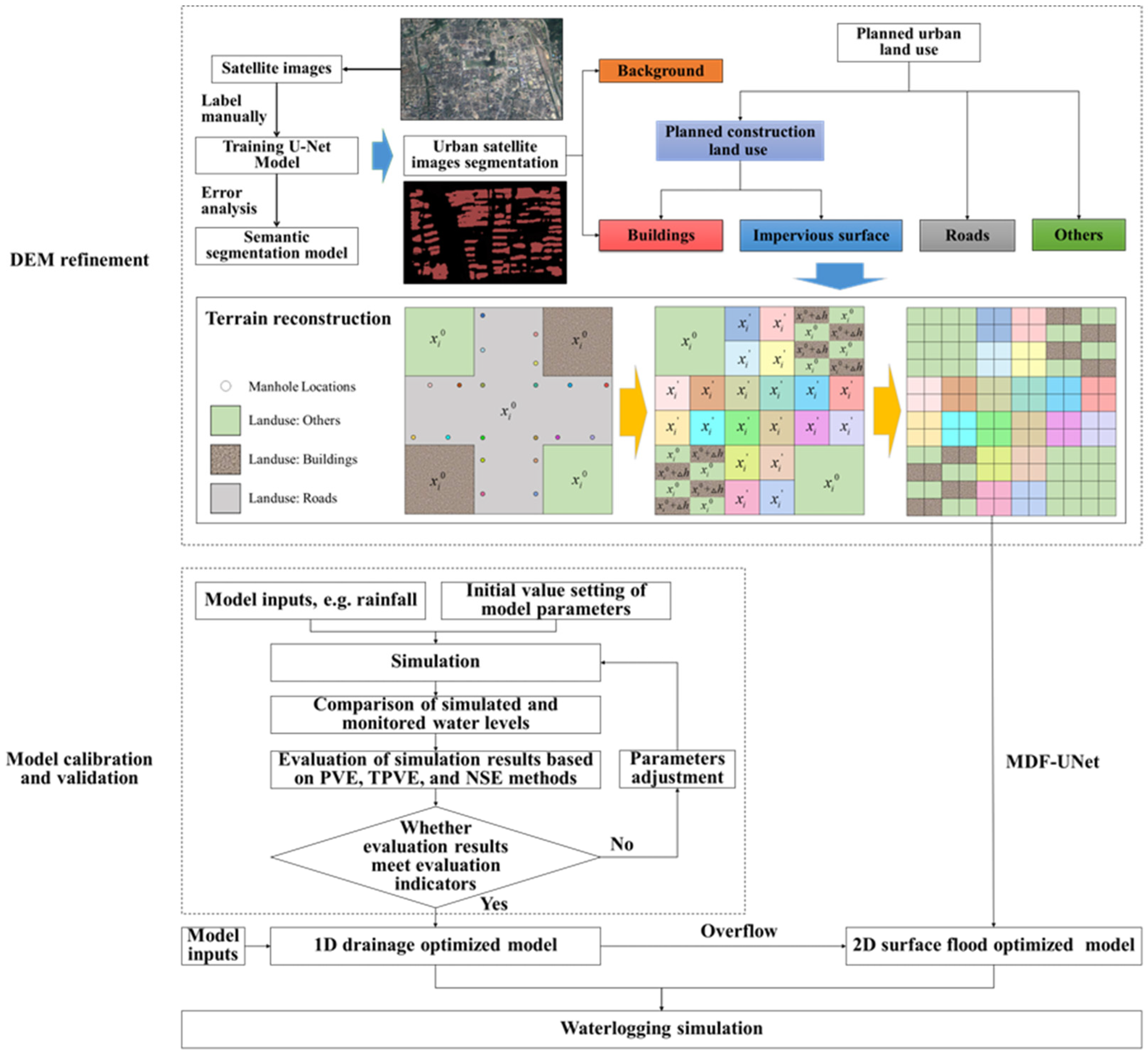
2. Methodology
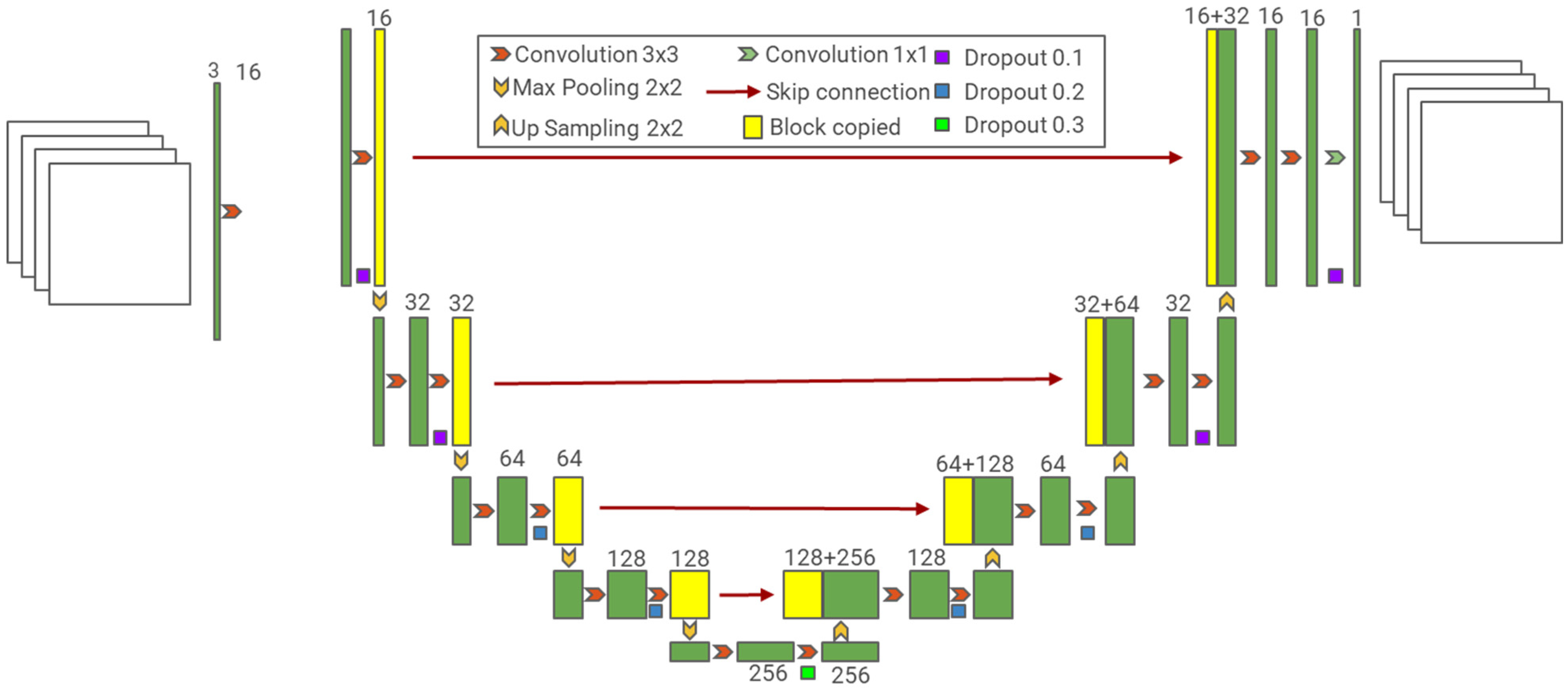
2.1. U-Net Model for Segmentation
2.2. Topographic Reconstruction Model
2.3. Hydrological and Hydrodynamic Model
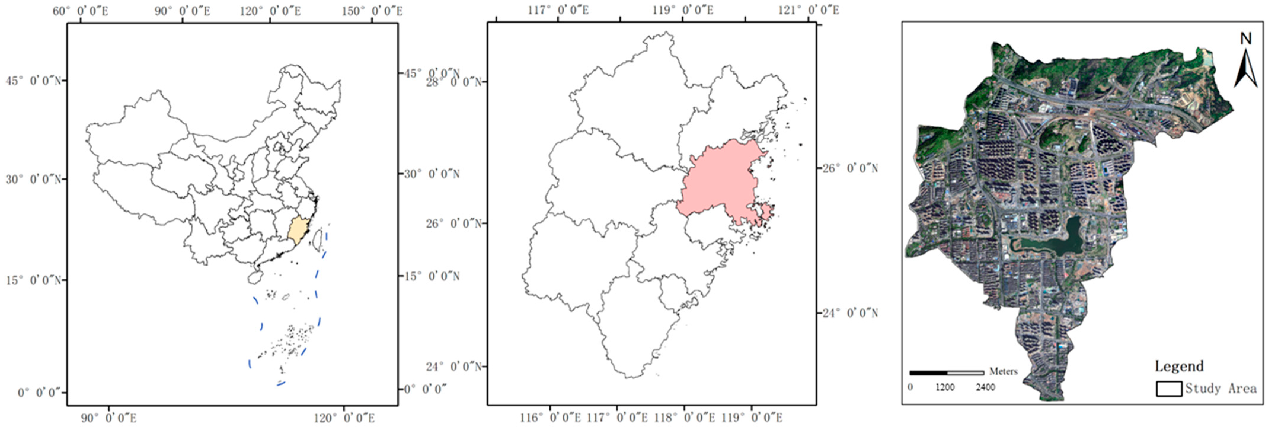
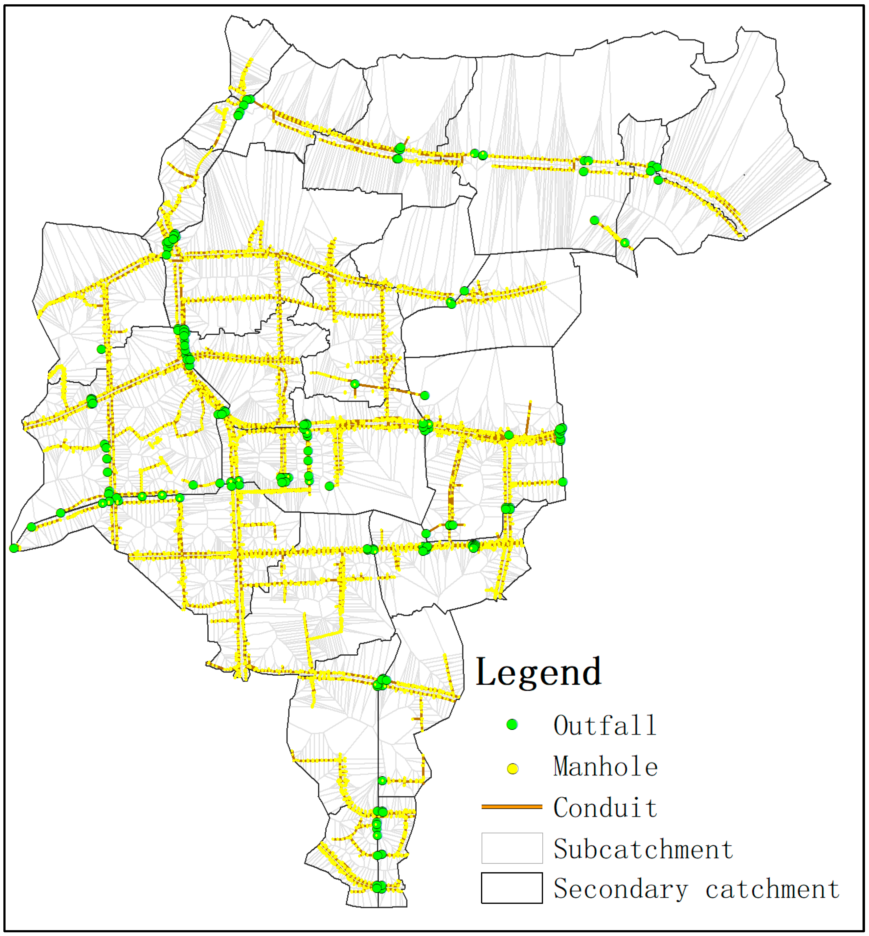
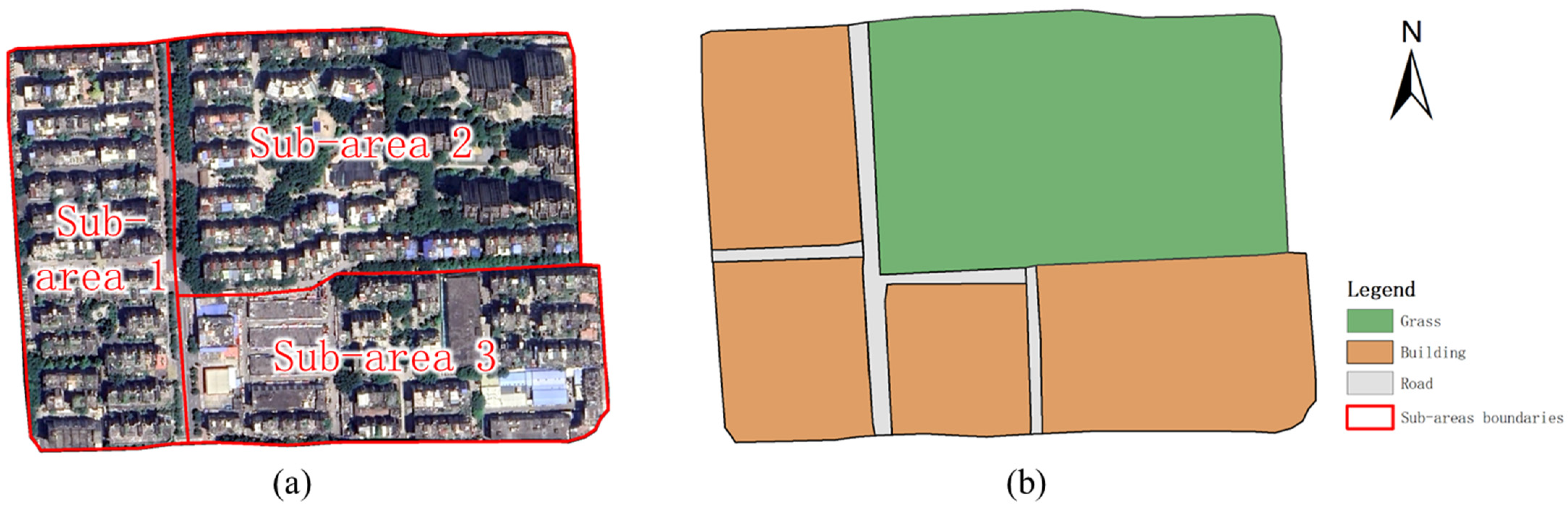
3. Study Area and Data Source
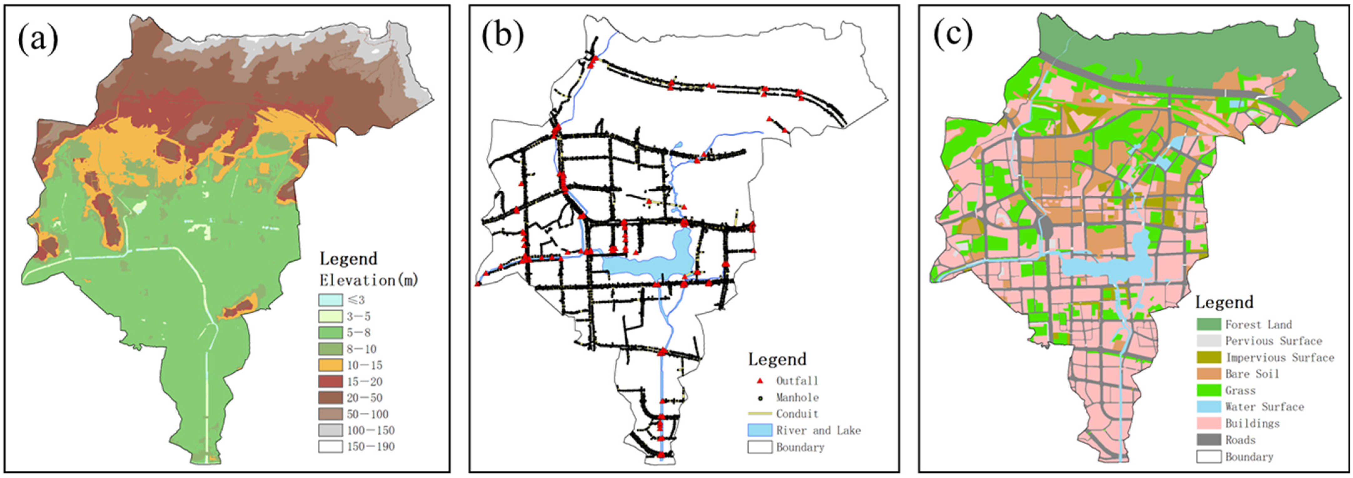
3.1. Data
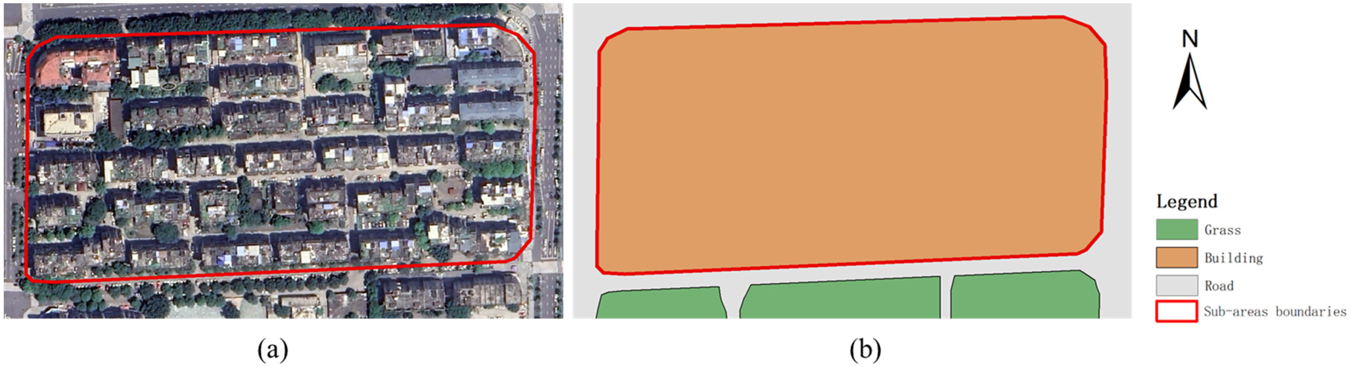
3.2. Building Area Segmentation Using U-Net Model
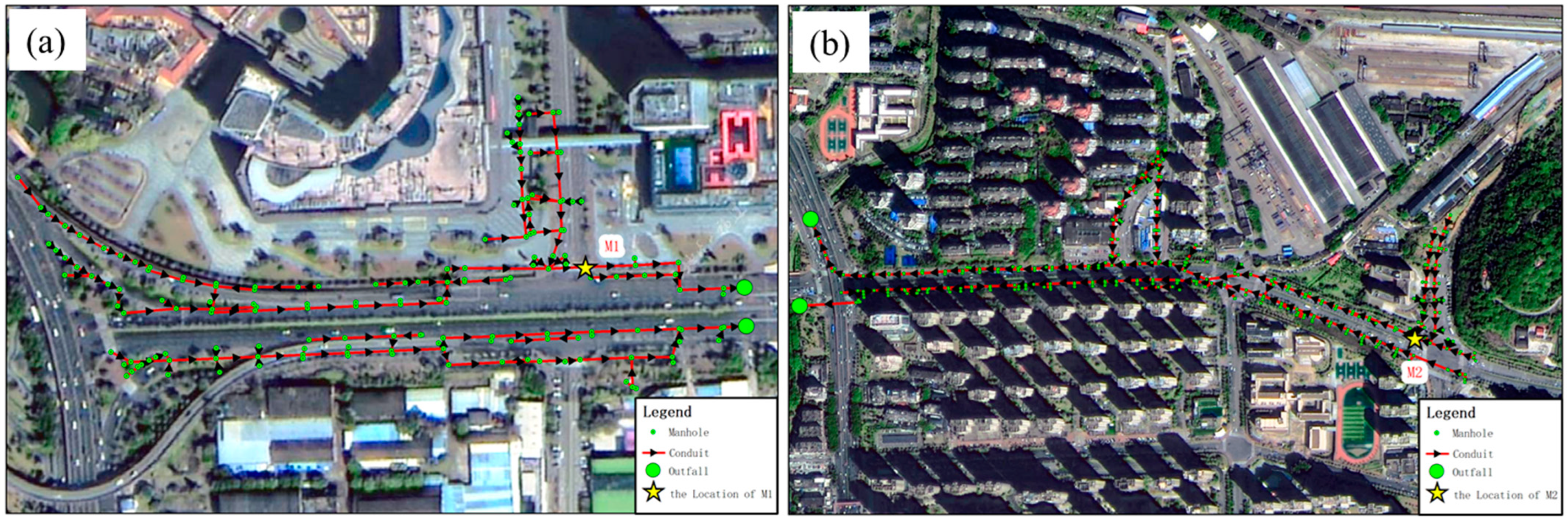
3.3. Model Construction
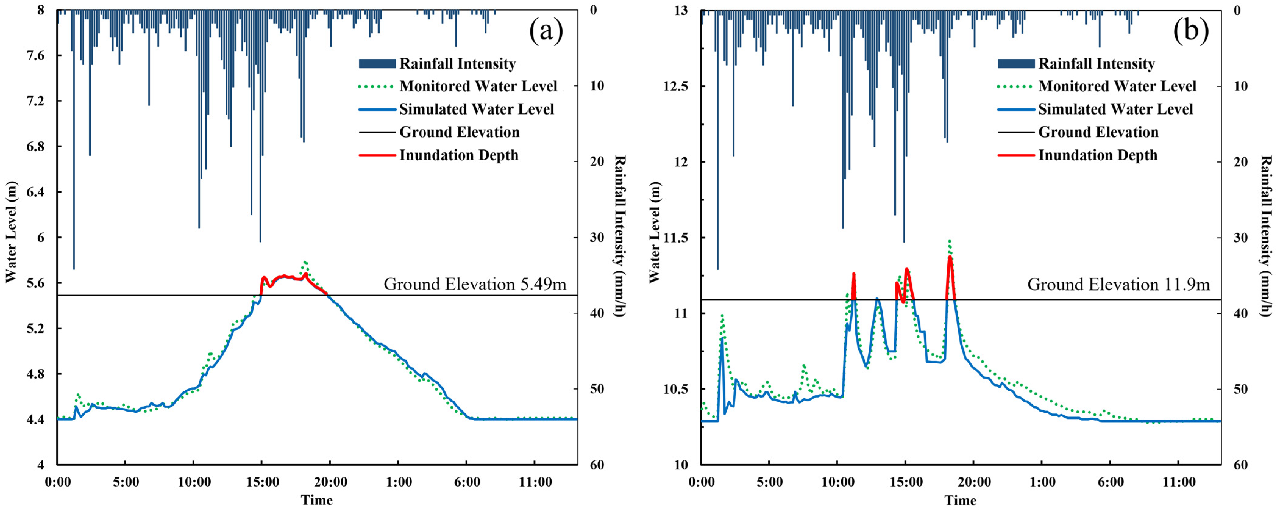
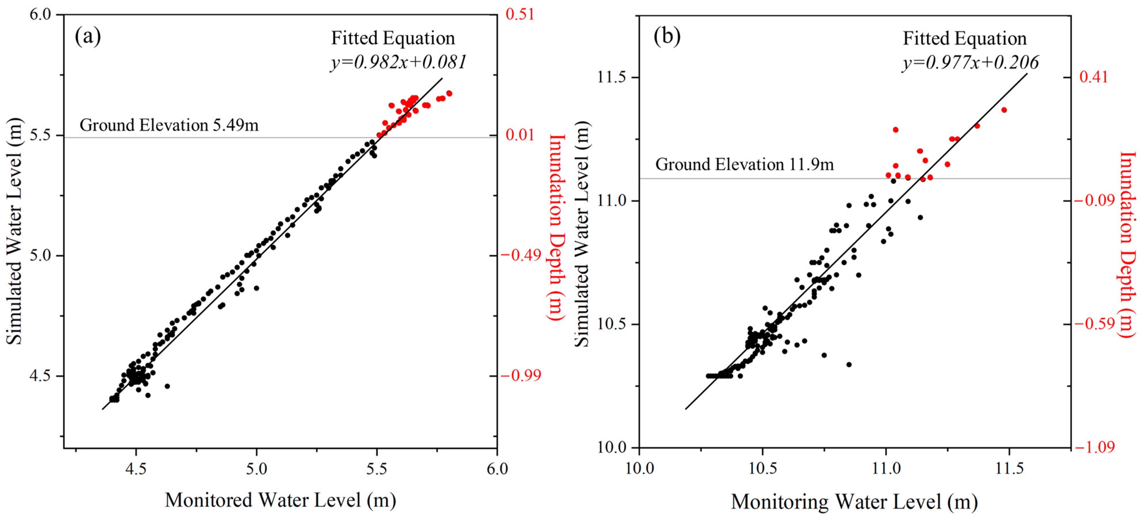
3.4. Model Calibration and Evaluation
4. Results and Discussions
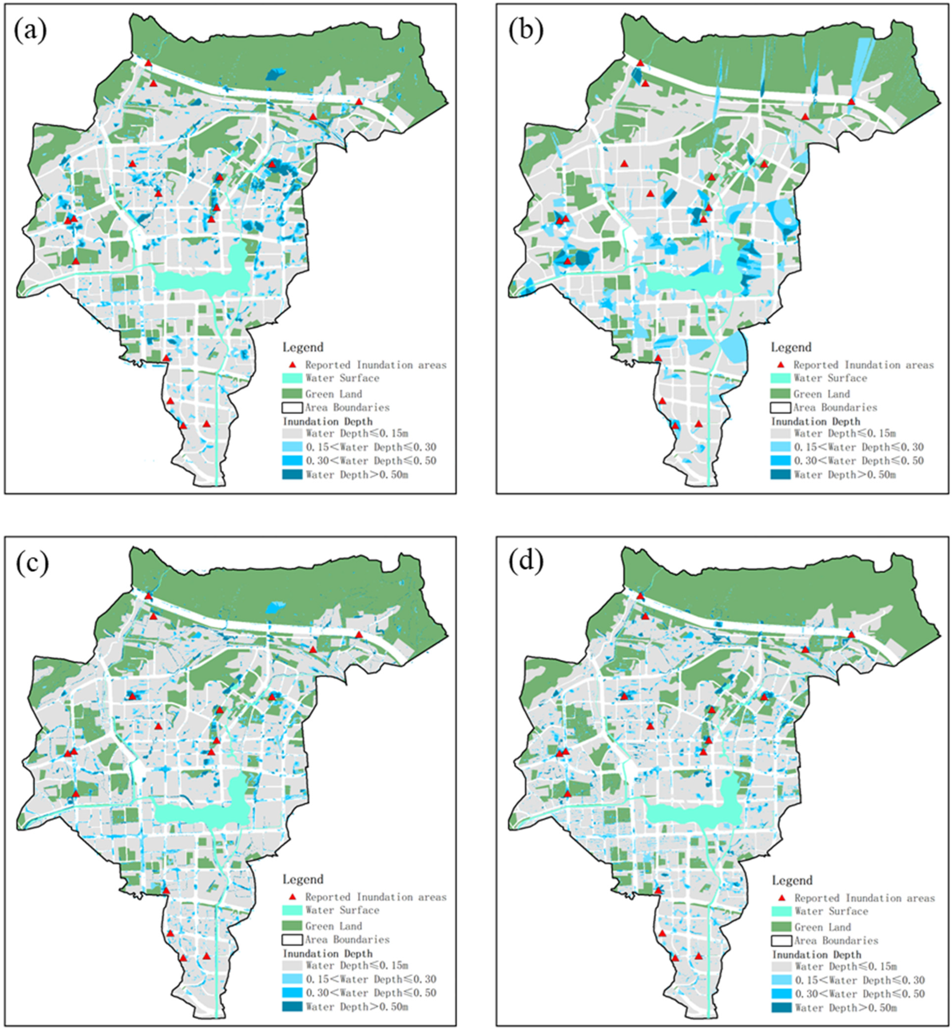
4.1. Overall Inundation Analysis
4.2. Inundated Areas Distribution on Roads
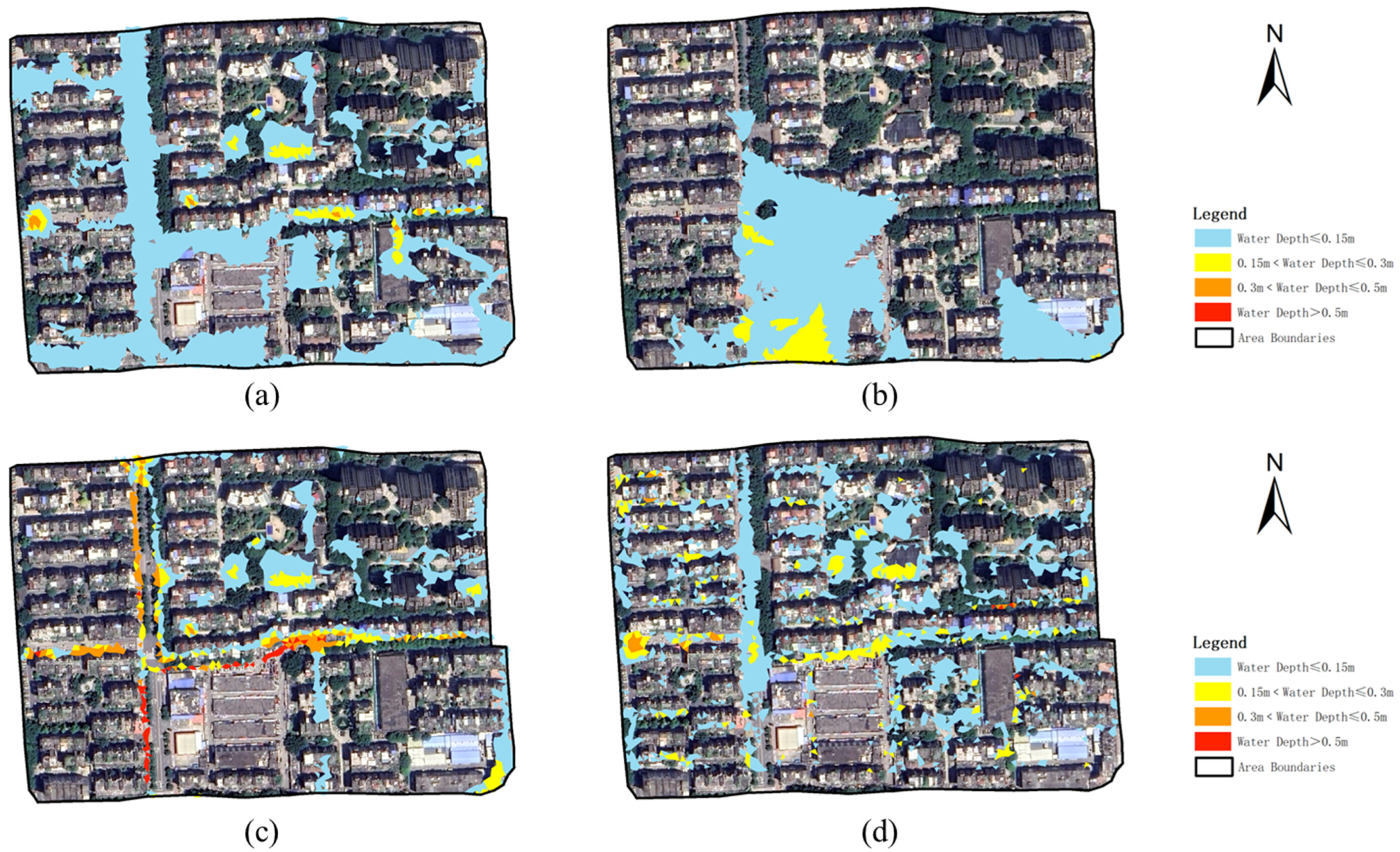
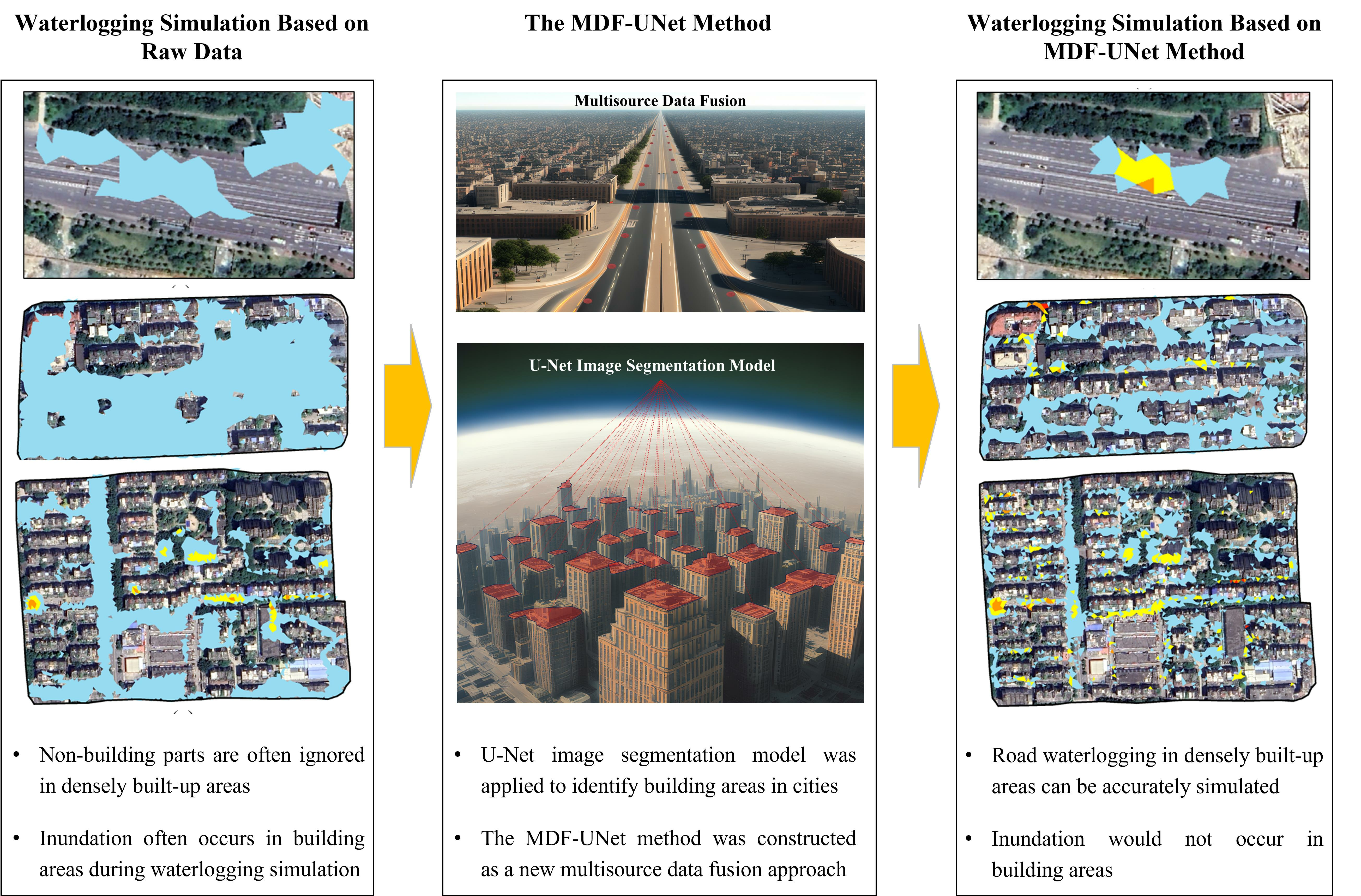
4.3. Inundated Areas Distribution in Densely Built-Up Areas
4.4. Limitations and Recommendations
5. Conclusions
- (1)
- The MDF-UNet method improved the simulation accuracy of urban waterlogging locations compared to the raw DEM data and the data from the IDW and MDF methods. Among the 17 historically recorded waterlogging points in the study area, 10 were simulated, while the number was 15 using the proposed method. The accuracy improved from 58.8% to 88.2%.
- (2)
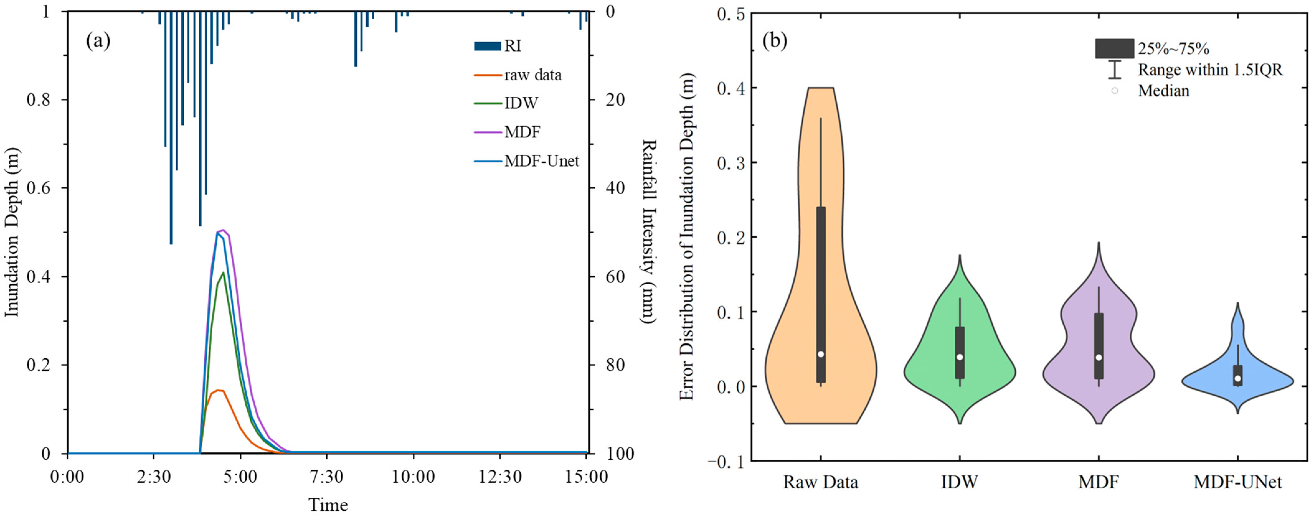
- The difference between the IDW, MDF, and MDF-UNet methods in the road waterlogging range simulation was small, without including the inundated depth. The ranking of maximum inundated depth obtained from different methods was MDF > MDF-UNet > IDW > raw DEM, and the median value errors of the first three methods are within 0.2 m compared with the raw DEM data of 0.4 m. This was due to the fact that the latter was not processed; hence, the accuracy could not meet the high data quality requirements for waterlogging simulation.
- (3)
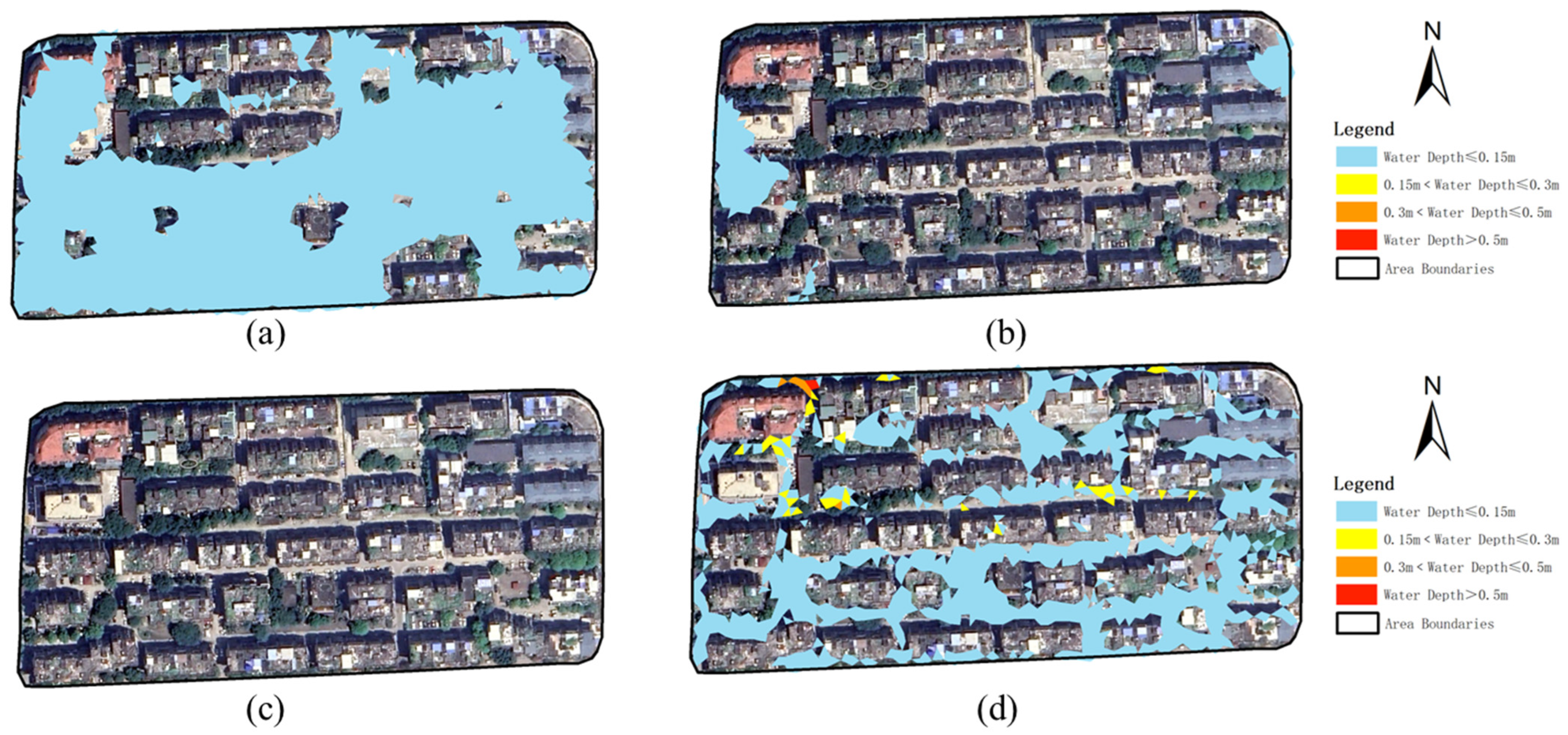
- The waterlogging model based on the MDF-UNet method was more compatible with the actual situation, especially in building locations, both in terms of inundated ranges and depths. The inundation ranges simulated by the raw DEM data, IDW and MDF-UNet methods were 32,722 m2, 3025 m2, and 9562 m2 in densely built-up Area 2, and the maximum inundated depths simulated by the same set of methods were 0.42 m, 0.28 m, 0.83 m, and 0.74 m in Area 3, respectively.
Author Contributions
Funding
Data Availability Statement
Conflicts of Interest
References
- Zhou, Y.; Wu, Z.; Xu, H.; Wang, H. Prediction and early warning method of inundation process at waterlogging points based on Bayesian model average and data-driven. J. Hydrol. Reg. Stud. 2022, 44, 101248. [Google Scholar]
- Jiang, J.; Liu, J.; Cheng, C.; Huang, J.; Xue, A. Automatic Estimation of Urban Waterlogging Depths from Video Images Based on Ubiquitous Reference Objects. Remote Sens. 2019, 11, 587. [Google Scholar] [CrossRef]
- Guo, Y.; Quan, L.; Song, L.; Liang, H. Construction of rapid early warning and comprehensive analysis models for urban waterlogging based on AutoML and comparison of the other three machine learning algorithms. J. Hydrol. 2022, 605, 127367. [Google Scholar]
- Huang, M.; Jin, S. A methodology for simple 2-D inundation analysis in urban area using SWMM and GIS. Nat. Hazards 2019, 97, 15–43. [Google Scholar]
- Chen, Z.; Li, K.; Du, J.; Chen, Y.; Liu, R.; Wang, Y. Three-dimensional simulation of regional urban waterlogging based on high-precision DEM model. Nat. Hazards 2021, 108, 2653–2677. [Google Scholar]
- Chen, Y.; Liu, R.; Barrett, D.; Gao, L.; Zhou, M.; Renzullo, L.; Emelyanova, I. A spatial assessment framework for evaluating flood risk under extreme climates. Sci. Total Environ. 2015, 538, 512–523. [Google Scholar]
- Hawker, L.; Bates, P.; Neal, J.; Rougier, J. Perspectives on Digital Elevation Model (DEM) Simulation for Flood Modeling in the Absence of a High-Accuracy Open Access Global DEM. Front. Earth Sci. 2018, 6, 233. [Google Scholar]
- Zhang, Q.; Wu, Z.; Guo, G.; Zhang, H.; Tarolli, P. Explicit the urban waterlogging spatial variation and its driving factors: The stepwise cluster analysis model and hierarchical partitioning analysis approach. Sci. Total Environ. 2021, 763, 143041. [Google Scholar]
- Omar, H.; Fizazi, H.; Faouzi, B.; Djemoui, C.; Lahcen, W.K. High-resolution DEM building with SAR interferometry and high-resolution. IET Image Process. 2019, 13, 713–721. [Google Scholar]
- Rajakumari, S.; Mahesh, R.; Sarunjith, K.J.; Ramesh, R. Volumetric change analysis of the Cauvery delta topography using radar remote sensing. Egypt. J. Remote Sens. Space Sci. 2022, 25, 687–695. [Google Scholar]
- Muhadi, N.A.; Abdullah, A.F.; Bejo, S.K.; Mahadi, M.R.; Mijic, A. The Use of LiDAR-Derived DEM in Flood Applications: A Review. Remote Sens. 2020, 12, 2308. [Google Scholar]
- Rehman, K.; Fareed, N.; Chu, H. NASA ICESat-2: Space-Borne LiDAR for Geological Education and Field Mapping of Aeolian Sand Dune Environments. Remote Sens. 2023, 15, 2882. [Google Scholar]
- Su, Y.; Guo, Q.; Ma, Q.; Li, W. SRTM DEM Correction in Vegetated Mountain Areas through the Integration of Spaceborne LiDAR, Airborne LiDAR, and Optical Imagery. Remote Sens. 2015, 7, 11202–11225. [Google Scholar]
- Wani, Z.M.; Nagai, M. An approach for the precise DEM generation in urban environments using multi-GNSS. Measurement 2021, 177, 109311. [Google Scholar]
- Zaidi, S.M.; Akbari, A.; Gisen, J.I.; Kazmi, J.H.; Gul, A.; Fhong, N.Z. Utilization of Satellite-based Digital Elevation Model (DEM) for Hydrologic Applications: A Review. J. Geol. Soc. India 2018, 92, 329–336. [Google Scholar]
- Boucher, C.; Noyer, J. A General Framework for 3-D Parameters Estimation of Roads Using GPS, OSM and DEM Data. Sensors 2018, 18, 41. [Google Scholar] [CrossRef]
- Kholia, N.; Kotlia, B.S.; Joshi, N.; Kandregula, R.S.; Kothyari, G.C.; Dumka, R.K. Quantitative analysis of Khajjiar and Rewalsar lakes and their surroundings, Himachal Pradesh (India): Remote sensing and GIS-based approaches. J. Appl. Geophys. 2023, 211, 104976. [Google Scholar]
- Mercer, A. A DEM of the 2010 surface topography of Storglaciären, Sweden. J. Maps. 2016, 12, 1112–1118. [Google Scholar]
- Jawak, S.D.; Luis, A.J. Synergistic use of multitemporal RAMP, ICESat and GPS to construct an accurate DEM of the Larsemann Hills region, Antarctica. Adv. Space Res. 2012, 50, 457–470. [Google Scholar] [CrossRef]
- Ebrahim, P.K.; Ramachandra, S.; Javier, I.; Subhro, G. Digital Modeling of Construction Site Terrain Using Remotely Sensed Data and Geographic Information Systems Analyses. J. Constr. Eng. Manag. 2014, 140, 04013067. [Google Scholar]
- Ahmad, I. Digital elevation model (DEM) coupled with geographic information system (GIS): An approach towards erosion modeling of Gumara watershed, Ethiopia. Environ. Monit. Assess. 2018, 190, 568. [Google Scholar] [CrossRef] [PubMed]
- Saksena, S.; Merwade, V. Incorporating the effect of DEM resolution and accuracy for improved flood inundation mapping. J. Hydrol. 2015, 530, 180–194. [Google Scholar] [CrossRef]
- Wang, Y.; Jiangxia, Y.; Chuan, C.; Zhou, R. Automated geometric precise correction of medium remote sensing images based on ASTER global digital elevation model. Geocarto Int. 2023, 38, 2190624. [Google Scholar] [CrossRef]
- Kaliappan, S.; Venkatraman, V. Determination of parameters for watershed delineation using various satellite derived digital elevation models and its accuracy. Glob. Nest J. 2023, 25, 124–137. [Google Scholar]
- Hojo, A.; Avtar, R.; Nakaji, T.; Tadono, T.; Takagi, K. Modeling forest above-ground biomass using freely available satellite and multisource datasets. Ecol. Inform. 2023, 74, 101973. [Google Scholar] [CrossRef]
- Okolie, C.J.; Smit, J.L. A systematic review and meta-analysis of Digital elevation model (DEM) fusion: Pre-processing, methods and applications. ISPRS J. Photogramm. 2022, 188, 1–29. [Google Scholar] [CrossRef]
- Tran, T.; Nguyen, B.Q.; Vo, N.D.; Le, M.; Nguyen, Q.; Lakshmi, V.; Bolten, J.D. Quantification of global Digital Elevation Model (DEM)—A case study of the newly released NASADEM for a river basin in Central Vietnam. J. Hydrol. Reg. Stud. 2023, 45, 101282. [Google Scholar] [CrossRef]
- Huang, J.; Wei, L.; Chen, T.; Luo, M.; Yang, H.; Sang, Y. Evaluation of DEM Accuracy Improvement Methods Based on Multi-Source Data Fusion in Typical Gully Areas of Loess Plateau. Sensors 2023, 23, 3878. [Google Scholar] [CrossRef]
- Hong Hu, G.Z.J.A. Multi-information PointNet++ fusion method for DEM construction from airborne LiDAR data. Geocarto Int. 2022, 38, 2153929. [Google Scholar]
- Wang, H.; Lei, X.; Wang, C.; Liao, W.; Kang, A.; Huang, H.; Ding, X.; Chen, Y.; Zhang, X. A coordinated drainage and regulation model of urban water systems in China: A case study in Fuzhou city. River 2023, 2, 5–20. [Google Scholar] [CrossRef]
- Patel, A.; Jena, P.P.; Khatun, A.; Chatterjee, C. Improved Cartosat-1 Based DEM for Flood Inundation Modeling in the Delta Region of Mahanadi River Basin, India. J. Indian Soc. Remote 2022, 50, 1227–1241. [Google Scholar] [CrossRef]
- Li, T.; Fan, J.; Liu, Y.; Lu, R.; Hou, Y.; Lu, J. An Improved Independent Parameter Decomposition Method for Gaofen-3 Surveying and Mapping Calibration. Remote Sens. 2022, 14, 3089. [Google Scholar] [CrossRef]
- Chen, H.; Liang, Q.; Liu, Y.; Xie, S. Hydraulic correction method (HCM) to enhance the efficiency of SRTM DEM in flood modeling. J. Hydrol. 2018, 559, 56–70. [Google Scholar] [CrossRef]
- Noh, M.; Howat, I.M. Automatic relative RPC image model bias compensation through hierarchical image matching for improving DEM quality. ISPRS J. Photogramm. 2018, 136, 120–133. [Google Scholar] [CrossRef]
- Schlund, M.; von Poncet, F.; Wessel, B.; Schweisshelm, B.; Kiefl, N. Assessment of TanDEM-X DEM 2020 Data in Temperate and Boreal Forests and Their Application to Canopy Height Change. PFG—J. Photogramm. Remote Sens. Geoinf. Sci. 2023, 91, 107–123. [Google Scholar] [CrossRef]
- Wang, R.; Lv, X.; Chai, H.; Zhang, L. A Three-Dimensional Block Adjustment Method for Spaceborne InSAR Based on the Range-Doppler-Phase Model. Remote Sens. 2023, 15, 1046. [Google Scholar] [CrossRef]
- Arefi, H.; Reinartz, P. Accuracy Enhancement of ASTER Global Digital Elevation Models Using ICESat Data. Remote Sens. 2011, 3, 1323–1343. [Google Scholar] [CrossRef]
- Guan, L.; Hu, J.; Pan, H.; Wu, W.; Sun, Q.; Chen, S.; Fan, H. Fusion of public DEMs based on sparse representation and adaptive regularization variation model. ISPRS J. Photogramm. 2020, 169, 125–134. [Google Scholar] [CrossRef]
- Wang, S.; Ren, Z.; Wu, C.; Lei, Q.; Gong, W.; Ou, Q.; Zhang, H.; Ren, G.; Li, C. DEM generation from Worldview-2 stereo imagery and vertical accuracy assessment for its application in active tectonics. Geomorphology 2019, 336, 107–118. [Google Scholar] [CrossRef]
- Wu, Y.; Zhang, H.; Wang, J.; Wang, R.; Zhao, F.; Wu, Z.; Cai, Y. Stereo-Radargrammetry Assisted InSAR Phase Unwrapping Method for DEM Generation. IEEE Trans. Geosci. Remote 2022, 60, 1–18. [Google Scholar] [CrossRef]
- Liu, J.; Ma, S.; Chen, R. Exploring the Optimal 4D-SfM Photogrammetric Models at Plot Scale. Remote Sens. 2023, 15, 2269. [Google Scholar] [CrossRef]
- Ruan, X.; Cheng, L.; Chu, S.; Yan, Z.; Zhou, X.; Duan, Z.; Li, M. A new digital bathymetric model of the South China Sea based on the subregional fusion of seven global seafloor topography products. Geomorphology 2020, 370, 107403. [Google Scholar] [CrossRef]
- Aati, S.; Avouac, J. Optimization of Optical Image Geometric Modeling, Application to Topography Extraction and Topographic Change Measurements Using PlanetScope and SkySat Imagery. Remote Sens. 2020, 12, 3418. [Google Scholar] [CrossRef]
- Liu, J.; Shao, W.; Xiang, C.; Mei, C.; Li, Z. Uncertainties of urban flood modeling: Influence of parameters for different underlying surfaces. Environ. Res. 2020, 182, 108929. [Google Scholar] [CrossRef] [PubMed]
- Zhang, M.; Xu, M.; Wang, Z.; Lai, C. Assessment of the vulnerability of road networks to urban waterlogging based on a coupled hydrodynamic model. J. Hydrol. 2021, 603, 127105. [Google Scholar] [CrossRef]
- Tang, X.; Shu, Y.; Lian, Y.; Zhao, Y.; Fu, Y. A spatial assessment of urban waterlogging risk based on a Weighted Naïve Bayes classifier. Sci. Total Environ. 2018, 630, 264–274. [Google Scholar] [CrossRef]
- Qi, X.; Zhang, Z. Assessing the urban road waterlogging risk to propose relative mitigation measures. Sci. Total Environ. 2022, 849, 157691. [Google Scholar] [CrossRef]
- Chai, X.; Dong, Y.; Li, Y. Waterlogging Assessment of Chinese Ancient City Sites Considering Microtopography: A Case Study of the PuZhou Ancient City Site, China. Remote Sens. 2022, 14, 4417. [Google Scholar] [CrossRef]
- Marsh, C.B.; Harder, P.; Pomeroy, J.W. Validation of FABDEM, a global bare-earth elevation model, against UAV-lidar derived elevation in a complex forested mountain catchment. Environ. Res. Commun. 2023, 5, 31009. [Google Scholar] [CrossRef]
- Liu, Y.; Bates, P.D.; Neal, J.C. Bare-earth DEM generation from ArcticDEM and its use in flood simulation. Nat. Hazards Earth Syst. 2023, 23, 375–391. [Google Scholar] [CrossRef]
- Xing, Y.; Chen, H.; Liang, Q.; Ma, X. Improving the performance of city-scale hydrodynamic flood modelling through a GIS-based DEM correction method. Nat. Hazards 2022, 112, 2313–2335. [Google Scholar] [CrossRef]
- Liu, Y.; Bates, P.D.; Neal, J.C.; Yamazaki, D. Bare-Earth DEM Generation in Urban Areas for Flood Inundation Simulation Using Global Digital Elevation Models. Water Resour. Res. 2021, 57, e2020WR028516. [Google Scholar] [CrossRef]
- Wang, Y.; Meng, Q.; Qi, Q.; Yang, J.; Liu, Y. Region Merging Considering Within- and Between-Segment Heterogeneity: An Improved Hybrid Remote-Sensing Image Segmentation Method. Remote Sens. 2018, 10, 781. [Google Scholar] [CrossRef]
- Zhu, H.; Xu, Y.; Cheng, Y.; Liu, H.; Zhao, Y. Landform classification based on optimal texture feature extraction from DEM data in Shandong Hilly Area, China. Front. Earth Sci.-PRC. 2019, 13, 641–655. [Google Scholar] [CrossRef]
- Pally, R.J.; Samadi, S. Application of image processing and convolutional neural networks for flood image classification and semantic segmentation. Environ. Modell. Softw. 2022, 148, 105285. [Google Scholar] [CrossRef]
- Lee, J.; Kang, H. Flood fill mean shift: A robust segmentation algorithm. Int. J. Control. Autom. Syst. 2010, 8, 1313–1319. [Google Scholar] [CrossRef]
- Meadows, M.; Wilson, M. A Comparison of Machine Learning Approaches to Improve Free Topography Data for Flood Modelling. Remote Sens. 2021, 13, 275. [Google Scholar] [CrossRef]
- Wu, C.; Jia, W.; Yang, J.; Zhang, T.; Dai, A.; Zhou, H. Economic Fruit Forest Classification Based on Improved U-Net Model in UAV Multispectral Imagery. Remote Sens. 2023, 15, 2500. [Google Scholar] [CrossRef]
- Maurya, A.; Akashdeep; Mittal, P.; Kumar, R. A modified U-net-based architecture for segmentation of satellite images on a novel dataset. Ecol. Inform. 2023, 75, 102078. [Google Scholar] [CrossRef]
- Liang, Y.; Yin, F.; Xie, D.; Liu, L.; Zhang, Y.; Ashraf, T. Inversion and Monitoring of the TP Concentration in Taihu Lake Using the Landsat-8 and Sentinel-2 Images. Remote Sens. 2022, 14, 6284. [Google Scholar] [CrossRef]
- Huang, F.; Liu, D.; Tan, X.; Wang, J.; Chen, Y.; He, B. Explorations of the implementation of a parallel IDW interpolation algorithm in a Linux cluster-based parallel GIS. Comput. Geosci. 2011, 37, 426–434. [Google Scholar] [CrossRef]
- Bemporad, A. Active learning for regression by inverse distance weighting. Inf. Sci. 2023, 626, 275–292. [Google Scholar] [CrossRef]
- Tan, J.; Xie, X.; Zuo, J.; Xing, X.; Liu, B.; Xia, Q.; Zhang, Y. Coupling random forest and inverse distance weighting to generate climate surfaces of precipitation and temperature with Multiple-Covariates. J. Hydrol. 2021, 598, 126270. [Google Scholar] [CrossRef]
- Harman, B.I.; Koseoglu, H.; Yigit, C.O. Performance evaluation of IDW, Kriging and multiquadric interpolation methods in producing noise mapping: A case study at the city of Isparta, Turkey. Appl. Acoust. 2016, 112, 147–157. [Google Scholar] [CrossRef]
- Huang, H.; Liao, W.; Lei, X.; Wang, C.; Cai, Z.; Wang, H. An urban DEM reconstruction method based on multisource data fusion for urban pluvial flooding simulation. J. Hydrol. 2023, 617, 128825. [Google Scholar] [CrossRef]
- Gironás, J.; Roesner, L.A.; Rossman, L.A.; Davis, J. A new applications manual for the Storm Water Management Model (SWMM). Environ. Modell. Softw. 2010, 25, 813–814. [Google Scholar] [CrossRef]
- Wang, L.; Li, Y.; Hou, H.; Chen, Y.; Fan, J.; Wang, P.; Hu, T. Analyzing spatial variance of urban waterlogging disaster at multiple scales based on a hydrological and hydrodynamic model. Nat. Hazards 2022, 114, 1915–1938. [Google Scholar] [CrossRef]
- Li, Z.; Yang, T.; Xu, C.; Shi, P.; Yong, B.; Huang, C.; Wang, C. Evaluating the area and position accuracy of surface water paths obtained by flow direction algorithms. J. Hydrol. 2020, 583, 124619. [Google Scholar] [CrossRef]
- Haag, S.; Shokoufandeh, A. Development of a data model to facilitate rapid watershed delineation. Environ. Model. Softw. 2019, 122, 103973. [Google Scholar] [CrossRef]
- Mabrouk, M.; Haoying, H. Urban resilience assessment: A multicriteria approach for identifying urban flood-exposed risky districts using multiple-criteria decision-making tools (MCDM). Int. J. Disaster Risk Reduct. 2023, 91, 103684. [Google Scholar] [CrossRef]
- Riazi, M.; Khosravi, K.; Shahedi, K.; Ahmad, S.; Jun, C.; Bateni, S.M.; Kazakis, N. Enhancing flood susceptibility modeling using multi-temporal SAR images, CHIRPS data, and hybrid machine learning algorithms. Sci. Total Environ. 2023, 871, 162066. [Google Scholar] [CrossRef] [PubMed]


| Module | Parameter | Value Range | Optimized Value |
|---|---|---|---|
| Subcatchment | N-Imperv | 0.011~0.025 | 0.023 |
| N-Perv | 0.060~0.300 | 0.096 | |
| Dstore-Imperv (mm) | 2.00~4.00 | 2.75 | |
| Dstore-Perv (mm) | 2.50~10.00 | 4.81 | |
| Infiltration | Max. Infil. Rate (mm/h) | 30.00~90.00 | 75.32 |
| Min. Infil. Rate (mm/h) | 0.10~10.00 | 4.53 | |
| Decay Constant | 2.00~7.00 | 4.79 | |
| Drainage | Roughness | 0.010~0.030 | 0.016 |
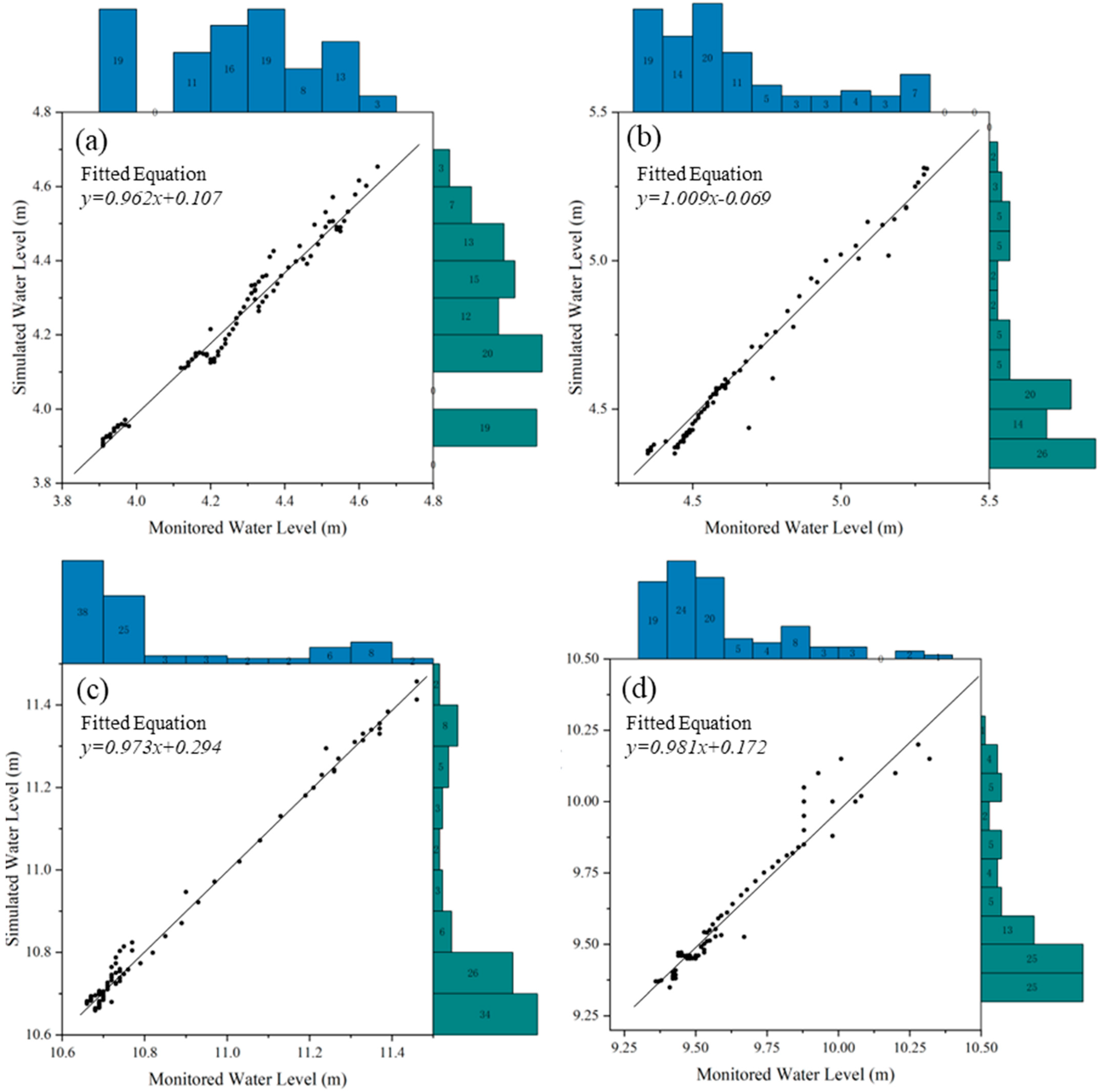
| NO. | WL | PV (m) | TPV | PVE (m) | TPVE (min) | NSE |
|---|---|---|---|---|---|---|
| M1 | MWL | 4.65 | 13:10 | 0.01 | 0 | 0.87 |
| SWL | 4.66 | 13:20 | ||||
| M2 | MWL | 8.28 | 14:00 | 0.05 | 10 | 0.88 |
| SWL | 8.33 | 13:50 | ||||
| M3 | MWL | 11.46 | 13:20 | 0.03 | 10 | 0.91 |
| SWL | 11.43 | 13:10 | ||||
| M4 | MWL | 10.32 | 13:30 | 0.11 | 20 | 0.79 |
| SWL | 10.21 | 13:10 |
| Raw DEM | IDW | MDF-UNet | MDF | |
|---|---|---|---|---|
| Inundated Area (m2) | 32,722 | 3025 | 9562 | / |
| Maximum Inundated Depth (m) | 0.12 | 0.14 | 0.56 | / |
| Raw DEM | IDW | MDF | MDF-UNet | |
|---|---|---|---|---|
| Inundated Area (m2) | 30,589 | 32,518 | 16,527 | 20,126 |
| Maximum Inundated Depth (m) | 0.42 | 0.28 | 0.83 | 0.74 |
Disclaimer/Publisher’s Note: The statements, opinions and data contained in all publications are solely those of the individual author(s) and contributor(s) and not of MDPI and/or the editor(s). MDPI and/or the editor(s) disclaim responsibility for any injury to people or property resulting from any ideas, methods, instructions or products referred to in the content. |
© 2023 by the authors. Licensee MDPI, Basel, Switzerland. This article is an open access article distributed under the terms and conditions of the Creative Commons Attribution (CC BY) license (https://creativecommons.org/licenses/by/4.0/).
Share and Cite
Yang, Q.; Huang, H.; Wang, C.; Lei, X.; Feng, T.; Zuo, X. Improving the Accuracy of Urban Waterlogging Simulation: A Novel Computer Vision-Based Digital Elevation Model Refinement Approach for Roads and Densely Built-Up Areas. Remote Sens. 2023, 15, 4915. https://doi.org/10.3390/rs15204915
Yang Q, Huang H, Wang C, Lei X, Feng T, Zuo X. Improving the Accuracy of Urban Waterlogging Simulation: A Novel Computer Vision-Based Digital Elevation Model Refinement Approach for Roads and Densely Built-Up Areas. Remote Sensing. 2023; 15(20):4915. https://doi.org/10.3390/rs15204915
Chicago/Turabian StyleYang, Qiu, Haocheng Huang, Chao Wang, Xiaohui Lei, Tianyu Feng, and Xiangyang Zuo. 2023. "Improving the Accuracy of Urban Waterlogging Simulation: A Novel Computer Vision-Based Digital Elevation Model Refinement Approach for Roads and Densely Built-Up Areas" Remote Sensing 15, no. 20: 4915. https://doi.org/10.3390/rs15204915
APA StyleYang, Q., Huang, H., Wang, C., Lei, X., Feng, T., & Zuo, X. (2023). Improving the Accuracy of Urban Waterlogging Simulation: A Novel Computer Vision-Based Digital Elevation Model Refinement Approach for Roads and Densely Built-Up Areas. Remote Sensing, 15(20), 4915. https://doi.org/10.3390/rs15204915