Abstract
Radar automatic target recognition based on high-resolution range profile (HRRP) has become a research hotspot in recent years. The current works mainly focus on closed set recognition, where all the test samples are assigned to the training classes. However, radar may capture many unknown targets in practical applications, and most current methods are incapable of identifying the unknown targets as the ’unknown’. Therefore, open set recognition is proposed to solve this kind of recognition task. This paper analyzes the basic classification principle of both recognitions and makes sure that determining the closed classification boundary is the key to addressing open set recognition. To achieve this goal, this paper proposes a novel boundary detection algorithm based on the distribution balance property of k-nearest neighbor objects, which can be used to realize the identification of the known and unknown targets simultaneously by detecting the boundary of the known classes. Finally, extensive experiments based on measured HRRP data have demonstrated that the proposed algorithm is indeed helpful to greatly improve the open set performance by determining the closed classification boundary of the known classes.
1. Introduction
A high-resolution range profile (HRRP) is a one-dimensional distribution of a target’s scattering centers along the radar line of sight, which has abundant geometrical structure information that can be used to identify the target. Thus, radar automatic target recognition (RATR) based on HRRP has attracted much attention in recent years.
The current methods mainly perform closed set recognition (CSR), such as [1,2,3,4,5], where all the test samples are assigned to the training classes. However, radar may encounter many unknown targets in the practical applications of RATR. When the unknown targets are captured, the current CSR models are incapable of identifying these targets as the ‘unknown’. Instead, these models will misjudge them as the known classes, which can be shown in Figure 1a. Obviously, this kind of classification could seriously affect the accuracy of RATR. Therefore, open set recognition (OSR, [6]) is proposed to solve this kind of recognition task that needs to identify the ‘unknown’ targets at the same time as classification.
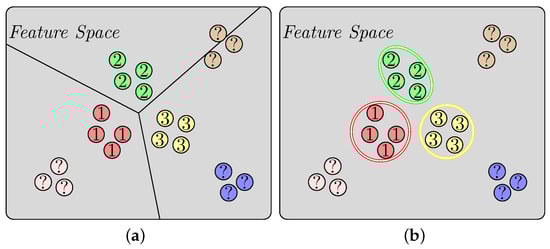
Figure 1.
This figure shows the basic classification principle of CSR and OSR. Obviously, the half-open classification boundary in the CSR model cannot handle the open set problem, and the closed classification boundary is more suitable for OSR. (a) CSR, (b) OSR.
As shown in Figure 1a, it is the half-open classification boundary that causes the classification error in an open set environment. Naturally, if we can determine a closed classification boundary for every known class, as shown in Figure 1b, then the sample inside the boundary will be classified as the corresponding known class, and the sample outside all the boundaries will be identified as an unknown class. Therefore, how to determine the specific closed classification boundary is the key to addressing the OSR problems.
There are some HRRP OSR works. According to the different ways of feature extraction, the existing methods can be mainly classified into two categories, i.e., traditional machine learning methods and deep learning methods.
The first category of methods is mainly based on support vector machine (SVM), support vector data description (SVDD), and random forest method. The authors of Chai et al. [7] proposed multi-kernel SVDD to describe the multi-mode distribution of HRRP; Zhang et al. [8] proposed a multi-classifier combination algorithm based on maximum correlation classifier, SVM, and relevance vector machine; Wang et al. [9] incorporated the extreme value theory into the random forest classifier for HRRP OSR. In addition, there are also some SVM-based methods focusing on public image datasets, such as 1-vs-set machine [6], -SVM [10], one class SVM (OCSVM, [11]), and W-SVM [12] methods. Among them, [13] evaluated the performance of -SVM on HRRP, and [14] evaluated the performance of two other SVM-based methods on MSTAR datasets. Among these methods, only SVDD can determine the closed classification boundary. Apart from the lack of determining the closed classification boundary, using the specific kernel function to extract distinguishable features may also limit the performance of these methods. With the development of deep learning, the methods based on the deep neural network have replaced these traditional machine learning methods.
The second category of methods mainly includes two kinds of models: discriminative models and generative models. The former focuses on proposing novel network architecture [15,16] and discriminative strategies [17,18,19,20,21,22] to extract more distinguishable features. Such as [16], Ma et al. [16] added another full-connection network branch to the end of the discriminator in the generative adversarial network (GAN, [23]), so the network structure has the ability to accomplish both classifying the known and identifying the unknown in synthetic aperture radar OSR. Zhang et al. [17] proposed a novel algorithm for open and imbalanced HRPP recognition tasks by learning from realistic data distribution and optimizing the accuracy over the majority, minority, and open classes.
In addition, there are some prototype learning-based methods that have achieved good performance on public image datasets, such as generalized convolutional prototype learning (GCPL, [24,25]), reciprocal points learning (RPL, [26]), and adversarial reciprocal points learning (ARPL, [27]). In prototype learning-based methods, the compactness of known features is usually improved to obtain more distinguishable features. Moreover, the distance between the sample and the prototype is used to evaluate the probability of belonging to the corresponding category, so this distance can be used to determine the closed classification boundary.
Different from discriminative models, new samples are generated in the training phase of generative models, and these samples are usually added into the training phase for better performance. Generally, the reconstruction error of the test sample is an important principle to identify the unknown classes in generative models, whose idea is similar to auto-encoder (AE, [28]). There are some representatives of generative models, such as [29,30,31,32]. In general, except for prototype learning-based methods, these deep learning methods almost ignore the importance of the closed classification boundary, which may limit their performance.
To fill the gap of the current methods, this paper proposes a novel boundary detection algorithm based on the distribution balance property of k-nearest neighbor objects (k-NNs). According to the theory of pattern recognition, a well-trained network can distinguish the known classes well and form stable clusters with clear boundaries in the feature space. Generally, the center points of these clusters are more densely distributed, while the boundary points are more sparsely distributed. Therefore, the k-NNs of a central point are more evenly distributed than that of a boundary point, which can be used to determine whether a point is a center point or a boundary point. Specifically, the proposed method calculates the distribution equilibrium coefficient and distance correction coefficient of a point based on its k-NNs to judge where it belongs, which are used to address the OSR problem in this paper. Finally, extensive experiments based on measured HRRP data are performed to evaluate the OSR performance of the proposed method, and the results verify the effectiveness of the proposed method.
The rest of this paper is organized as follows. Section 2 gives the general definition of OSR. In Section 3, the proposed method is described in detail. The experimental results based on measured data, as well as the comparison to some other methods, are discussed in Section 4. Finally, Section 5 concludes this paper.
2. Materials
To help our readers to further understand the OSR problems, this section gives the general definition of OSR.
Given a training set , the label of training sample belongs to . As for the test set , it contains two parts: the known classes and the unknown class . Specifically, the sample of and training set have the same category . All samples in belong to category, which represents ‘unknown’. All raw samples come from m-dimensional full space , so OSR aims to determine a mapping function based on , which can be expressed as
where represents the known samples of class j. As introduced in Section 1, OSR needs to not only classify the known classes, but also identify the unknown classes, which correspond to the 1st and 2nd line of Equation (1), respectively.
3. Methods
The flow diagram of the proposed method for HRRP OSR is shown in Figure 2. First, all raw HRRP samples need to be preprocessed to obtain the standardized training and test set. In the training phase, the preprocessed training data are used to train the network, which is a CSR training process. The trained network extracts the high-dimensional features from all training data, which are also called the known features or training features. After the training phase, this paper detects the closed classification boundary of these known features, which is the core of the proposed method. In the test phase, the specific category of the test features will be identified according to the closed classification boundary detected by the proposed method. Additionally, this paper hardly restricts the specific form of the loss function. In other words, the proposed method can be used in combination with a variety of CSR or OSR loss functions, which demonstrates the wide applicability of the proposed method.
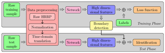
Figure 2.
The flow diagram of the proposed method for HRRP OSR.
3.1. Data Preprocessing
The way the radar acquires the HRRP data of the target determines the intensity sensitivity and translation sensitivity of the HRRP data. Therefore, the data preprocessing mainly aims at extinguishing both sensitivities.
3.1.1. Intensity Sensitivity
According to the working process of the radar, radar transmit power, target distance, radar antenna gain, radar receiver gain, and some other factors can affect the intensity of HRRP data, which indicates that the intensity may vary from target to target. Therefore, to avoid the recognition model taking the intensity information as the basis for judging the category of the target, normalization is usually used to eliminate the intensity sensitivity of the HRRP data. Specifically, normalization is used to process the raw HRRP data , which can be expressed as
where represents the norm of the raw data .
3.1.2. Translation Sensitivity
HRRP data are obtained from the echo signal intercepted by the sliding range window. The sliding of this distance window will affect the support area of HRRP data. Therefore, to avoid the influence of the sliding support area on the recognition result, it is necessary to carry out the corresponding translation operation on HRRP to obtain the standardized data. Specifically, this paper chooses the center of gravity self-alignment to eliminate translation sensitivity. The center of gravity of HRRP data can be expressed as
After several cyclic shifts, the center of gravity of HRRP can be moved to the center position . As shown in Figure 3, the support area of HRRP moves to the center position after preprocessing.
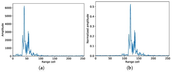
Figure 3.
Schematic diagram of the raw HRRP sample and preprocessed HRRP sample. After data preprocessing, the intensity sensitivity and translation sensitivity of HRRP data have been eliminated. (a) Raw HRRP, (b) Preprocessed HRRP.
3.2. Boundary Detection Algorithm
The boundary detection algorithm is the core of the proposed method, and this section gives a detailed introduction.
As shown in Figure 4a, the center of a cluster tends to have a denser distribution of points than the boundary of a cluster. In other words, the distribution of the center point’s k-NNs is more symmetric and balanced than that of the boundary point. Thus, a novel indicator, boundary detection coefficient (BDC), is proposed to describe the k-NNs’ distribution difference between the center point and the boundary point, which can be used to detect the boundary point of a cluster. Figure 4a visually shows the boundary detection results of the proposed method, whose distance distribution and BDC distribution can be seen in Figure 4b,c, respectively. Among them, a point with a larger BDC value is a boundary point.
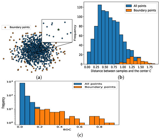
Figure 4.
The center point of a cluster, such as the ‘Star’ point in (a), its k-NNs are approximately uniformly distributed around it. In contrast, the k-NNs of the boundary point tend to be distributed on one side. In (a), the ‘Boundary points’ are the detection results from the proposed method. (b) shows the distance distribution in (a), and the center C is obtained by averaging all points. (c) shows the BDC distribution of all points in (c).
Given a set of points , the k-NNs of are denoted as
where is the j-th k-NNs of . In this paper, the balance of k-NN distribution is described by the distribution equilibrium coefficient () of , which can be expressed as the following formula:
where represents norm operation, and the tanh function is used to compress the range of into . Obviously, the better the balance of k-NN distribution, the smaller .
In fact, it is insufficient to use alone to distinguish the center and boundary point since it is possible that the k-NNs of a boundary point are distributed evenly. Nevertheless, the point distribution density of the center and boundary regions are still different, which can be used to further distinguish the center and boundary points. Specifically, this paper chooses the distance between k-NNs and the test point to describe this kind of density difference. Thus, a distance correction coefficient () is proposed to improve , which can be expressed as
where represents norm operation. Likewise, the better the balance of k-NNs distribution, the smaller .
In this paper, both and are used to describe the distribution balance of k-NNs, which can be expressed as
where is the proposed BDC. Obviously, the largest terms in are the boundary points of the cluster.
Next, we explain how to use BDC to detect the boundary points in the proposed OSR problem. Assuming that there are n samples in the training set , the training features can be denoted as
where is the embedding function of the trained network, and is the i-th training sample of the training set . Then, should be calculated to detect the boundary points of S, and the corresponding algorithm is shown in Algorithm 1. The calculation complexity of every procedure is also provided in Algorithm 1. It shows that the calculation complexity mainly depends on the detection procedure of the k-NNs, whose complexity is . Apart from the hyper-parameter k, there is another hyper-parameter that will affect the boundary detection results of the algorithm. This parameter determines the ratio of boundary points to all points, so its value is usually low, such as or . After all, there are only a few boundary points in the cluster.
| Algorithm 1 Boundary detection algorithm. |
|
3.3. Identification Procedure
This section discusses how to use the proposed boundary detection algorithm to identify the unknown classes.
After the training phase, the training features form N clusters with definite boundaries in the feature space, and the boundary points have been detected by the proposed method. At this time, for any test sample , what we need to do is to investigate the relationship between its embedding feature and the detected boundary in the feature space. Obviously, if the feature is outside the detected boundary, then should be classified as the unknown class. Conversely, if the feature is within the detected boundary, then should be recognized as a known class. As for how to judge whether feature is inside or outside the detected boundary, it is accomplished by the value of BDC of the proposed method. Specifically, if the BDC of feature , is greater than the BDC of the detected boundary, it is judged to be outside the boundary. The specific algorithm is shown in Algorithm 2.
| Algorithm 2 Identification algorithm. |
|
As shown in Algorithm 2, it gives all calculation processes of OSR with the proposed method and establishes a complete mapping function f from the raw data to the predicted label. In fact, the proposed method mainly focuses on how to identify the unknown classes while classifying the known classes requires additional operations. Specifically, when the test sample is identified as the known class, the 1st line of Equation (9) gives the specific predicted known class of , which is in . Although the core of the proposed method is based on the k-NN classification algorithm, the proposed method does not use the k-NNs of the test sample to determine its specific category. Instead, the proposed method determines the category of the sample feature by its distance from the feature center of the known cluster , which can be expressed as
where represents the center of the i-th known cluster, represents the number of i-th classes training samples, and represents the j-th training sample of i-th classes. It is believed that using the feature information of the whole category is more beneficial for classification than using the local k-NNs information.
4. Results and Discussion
4.1. Experimental Settings
4.1.1. Data
This paper conducts the OSR experiments on 13 kinds of measured airplane HRRP data, which are transmitted vertically and received vertically in linear polarization mode. Among them, An-26, Cessna, and Yak-42 are selected as the known classes, whose flight path and preprocessed HRRP are shown in Figure 5. The 1st column of Figure 5 shows the flight path of the known classes, which are cut into several segments. Specifically, the 5th and 6th segments of An-26, 6th and 7th segments of Cessna, and 2nd and 5th segments of Yak-42 are selected as the training samples, while the remaining segments are used as test samples. The reasons for such data division are as follows: first, the selected path can cover a relatively comprehensive flight attitude, which is conducive to avoiding the impact of target attitude on the recognition task; Second, the training data and the test data are not completely consistent, which is conducive to testing the generalization ability of the model. The 2nd column of Figure 5 shows that the support area width of three aircraft HRRP is different, which also reflects the size of the aircraft size from one side. Table 1 shows the number information on these three known classes. In addition, the remaining 10 kinds of aircraft each have 3000 samples, and they are used as the unknown classes for open set evaluating, whose specific category information can be seen in Section 4.4.
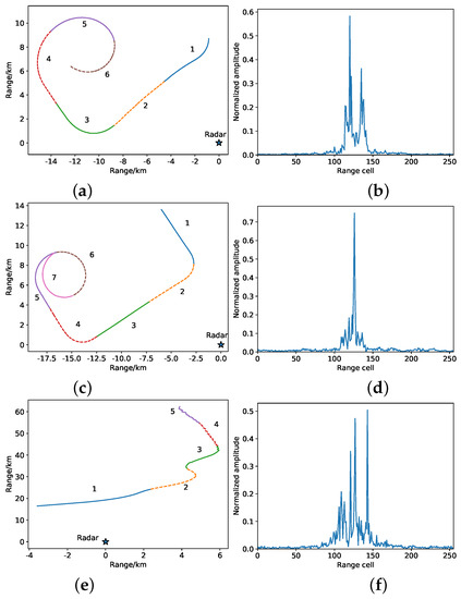
Figure 5.
This figure shows the flight path and preprocessed HRRP of three airplanes. (a) An−26; (b) An−26; (c) Cessna; (d) Cessna; (e) Yak−42; (f) Yak−42.

Table 1.
HRRP data of known classes overview.
4.1.2. Implementation Settings
This paper uses a simple one-dimensional convolutional neural network as the classifier, which has three convolutional layers and two fully-connected layers. In addition, the stochastic gradient descent-momentum optimizer is used to train the classifier for 100 epochs. The learning rate is set to and drops to one-tenth of the original after 30 epochs. The training batch size is set to 128.
4.2. Identification Evaluation
This experiment focuses on the ability of the model to identify the unknown classes. Thus, the area under the receiver operating characteristic curve (AUROC) is used to evaluate different methods. The specific experimental settings are shown in Section 4.1, and the results are shown in Table 2.
Table 2.
This table shows the experimental AUROC(%) results of various methods. Specifically, the 3rd, 4th, and 5th columns of this table are the experimental results of the proposed method combined with the corresponding loss function under parameter k. The best experimental results are shown in bold.
Obviously, when the proposed method is combined with different loss functions, the identification performance is greatly improved. In fact, the proposed method and other methods use the same feature extraction network. Thus, the performance improvement is entirely due to the boundary detection function of the proposed method, which strongly verifies the effectiveness of the proposed method. Moreover, the effect of parameter k on the performance of the proposed method is also investigated in this experiment. As shown in Table 2, except for SoftMax, the performance of the proposed method combined with other methods has slightly changed with the increases in parameter k. We speculate that this result may be related to the compactness of the feature clusters because all other methods have the ability to improve the compactness of the inter-class features. Moreover, receiver operating characteristic (ROC) curves of the proposed method combined with several loss functions are also presented, as shown in Figure 6, such as boundary detection SoftMax (BD_SoftMax), BD_ARPL, and BD_Ring. Finally, it is not certain which loss function combined with the proposed method will obtain the best performance, which is a limitation of the proposed method.
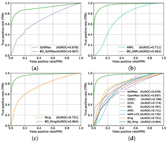
Figure 6.
This figure shows the ROC curve of some experimental results in Table 2. Among them, (a–c) intuitively demonstrate the performance improvement effect of the proposed method combined with the specific method, and (d) shows a comparison of the proposed method BD_Ring with the remaining methods. Moreover, parameter k in this figure is set to 5. (a) SoftMax; (b) ARPL; (c) Ring; (d) All methods.
4.3. Category Ablation Experiment
This experiment intends to investigate the performance change in the proposed method as the number in the unknown class increases gradually. Thus, 10 unknown classes are successively added to the test set for the category ablation experiment. In this experiment, macro average F1-score (F1) is used to evaluate the comprehensive performance of different methods, including the ability to classify the known classes and identify the unknown classes. Its expression is as follows:
where and represent the Precision and Recall of i-th category, respectively. The experimental results are shown in Figure 7. The horizontal axis of Figure 7 is openness [6], which can be expressed as
where is the number of known classes, is the number of test classes that includes the known and unknown classes, and is the number of known classes that need to be correctly recognized during testing. Obviously, the difficulty of OSR increases with increasing , so Figure 7 shows the performance of all methods decreases with increasing . Nevertheless, the proposed method still achieves the best performance when combined with the Ring loss function, as shown in Figure 7d. Moreover, the performance degradation rate of the proposed method is much lower than that of other methods, which further demonstrates that the proposed boundary detection method can effectively improve the OSR performance. Finally, this experiment shows that the proposed method can still obtain performance advantages in application scenarios with many unknown classes, which also verifies the effectiveness of the proposed method.
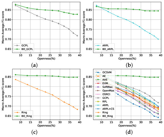
Figure 7.
(a–c) show the greatly improved performance of the proposed method in combination with the selected loss function under different , and (d) shows the performance comparison results between the various methods under different ; (a) GCPL; (b) ARPL; (c) Ring; (d) All methods.
4.4. Threshold Discussion
As is known, radar target detection need to set a specific detection threshold to judge whether there is a target in the echo. Specifically, when the echo intensity is higher than the threshold, it is considered that there is a target in the range window. When the echo intensity of the target is lower than the threshold, the radar will miss this target. Therefore, the setting of the detection threshold directly affects the results of target detection, which is very important in real applications. Similarly, the setting of thresholds also plays a significant role in OSR problems, which needs to determine a specific threshold for recognizing a test sample as a specific category in practical applications. Therefore, this section discusses how threshold affects the performance of the proposed method (Section 4.2 does not discuss the threshold because the evaluation of the metric AUROC is independent of the threshold in the proposed method).
Section 3.2 has introduced that represents the ratio of boundary points to all points. In other words, the identification process of the proposed method considers that only samples in the center ratio of known classes can be identified as ‘known’. Thus, it can be speculated that as increases, the ability of the model to recognize known classes increases. Nevertheless, when the value of is too low, the boundary range may be so large that it reduces the ability of the model to identify the unknown samples. Therefore, there may be an equilibrium point for the value of , which makes the comprehensive performance of the model reach its best. This phenomenon is the same as in radar target detection. If the detection threshold is set too high, fewer targets are detected and the higher the missed detection rate is. If the detection threshold is set too low, more targets are detected and the higher the false alarm rate will be. Therefore, there is an optimal detection threshold that can balance the missed detection rate and false alarm rate.
To explore the best threshold, this experiment examines the performance of different methods as a function of . Apart from the experimental settings in Section 4.1, parameter k is set to 5, and the experimental results are shown in Figure 8. As shown in Figure 8a–c, when the proposed method is combined with SoftMax and Ring, such as BD_SoftMax, BD_GCPL, and BD_Ring, the performance is greatly improved, which verifies the effectiveness of the proposed method. As expected, the performance of the model increases first and then decreases with the increase in the threshold . In addition, when the threshold increases to a certain extent, the performance of the proposed method suddenly decreases significantly, indicating that the threshold is close to the boundary of the feature cluster. Figure 8d shows that the proposed method BD_Ring achieves astonished performance among many methods.
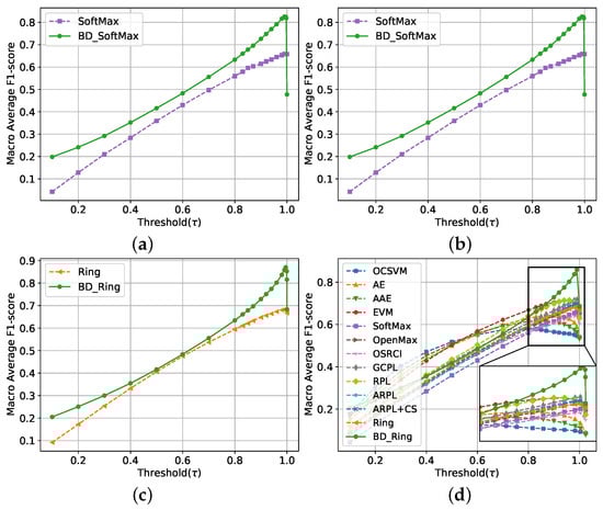
Figure 8.
This figure shows that the performance of the proposed method varies with the threshold . (a) SoftMax; (b) GCPL; (c) Ring; (d) All methods.
Moreover, Figure 9 shows several confusion matrices of BD_Ring with different thresholds . Obviously, with the increase in , fewer boundary points are detected by the proposed method, and the recognition ability of the proposed method for known classes is becoming stronger and stronger. At the same time, the ability of the proposed method to identify the unknown classes is slightly decreased with increasing threshold . Nevertheless, the proposed method can still effectively identify the unknown classes. Although the threshold is close to 1, there is still a gap between the recognition probability of the model for the known classes and 1, which is caused by the fact that the samples of the test set and the training set are incapable of completely meeting the same distribution. Taking ‘Cessna’ as an example, as shown in Figure 5c, the flight path data of the 6th and 7th segments are selected as the training set because it is believed that the circular flight path is considered to cover enough flight attitude. However, the attitude of the target is also related to the pitch angle of the target captured by the radar. Therefore, the target attitude of the flight path’s 6th and 7th segments is incapable of representing the target attitude of the other five flight paths, which results in the low classification rate of known classes in Figure 9. Additionally, these confusion matrices also show us that some unknown targets are easier to identify than others. Such as the class ‘CRJ-900’, even though the threshold has been selected as , the proposed model can still identify it with probability. By contrast, class ‘A320’ is more likely to be misjudged as ‘Yak-42’, which may result from the nature of the targets themselves.
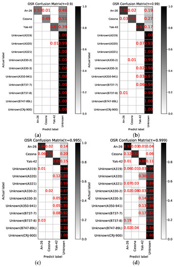
Figure 9.
This figure shows several confusion matrices when the proposed method is combined with the Ring loss function (BD_Ring). (a) = 0.9; (b) = 0.99; (c) = 0.995; (d) = 0.999.
4.5. Feature Visualization Analysis
This section gives more feature visualization results to better demonstrate the application of the proposed method in HRRP OSR.
The proposed method can identify not only the boundary points of two-dimensional clusters, as shown in Figure 4a, but also the boundary points of high-dimensional clusters. In our experiments, the features extracted from the network structure are all 128 dimensional features, which are difficult to be visualized directly. Therefore, this section visualizes the high-dimensional feature distribution by using the t-SNE [36] method to reduce the dimension. As shown in Figure 10a, the three known classes features can be well distinguished, while most of the unknown features can be distinguished except that a few of them overlap with the known features. In fact, the shape of known clusters can be extremely complex, especially when the dimension of the feature space is very high. Under this circumstance, it is naive and inappropriate to use the distance from the sample feature to the cluster center or to the prototype to determine the boundary points of a known cluster, which is why those prototype-based methods have poor performance, such as GCPL, RPL, and ARPL. For example, as shown in Figure 10b–d, although the proposed method can detect the boundary points of the known clusters, it is obviously difficult to identify the unknown samples based on the distance between the features of these boundary samples and the center of known clusters. In contrast, as shown in Figure 10e, the proposed method is much more reliable in identifying the unknown samples based on the BDC of the sample features. Compared with the known samples, the BDC distribution of the unknown samples is significantly higher. Therefore, it is easy to determine a BDC boundary to better distinguish between the known and unknown samples.
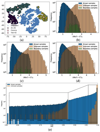
Figure 10.
This figure shows the feature distribution, distance distribution, and BDC distribution under the BD_Ring model of the proposed method. Among them, (a) shows the feature distribution after dimension reduction visualization by t-SNE, and the legends show the feature center of three known classes; (b–d) show the distance distribution from the sample features of three kinds of known targets and unknown features to the feature center; (e) shows the BDC distribution of the known and unknown features; (a) Feature distribution; (b) An−26; (c) Cessna; (d) Yak−42; (e) BDC distribution.
4.6. Computational Complexity
This section only discusses the computational complexity of the different methods in the test phase because the training phase of the model is not involved in practical applications. As for the training phase, Algorithm 1 has given more details.
First, the computational complexity of a deep learning algorithm is highly related to the network structure it uses. The larger and more complex the neural network structure is, the higher the computational complexity is. Therefore, this section does not discuss the computational complexity of using the network structure to extract the features, which corresponds to the 1st step in Algorithm 2. In fact, the proposed method in this step is the same as the other methods.
After extracting the test features, the decision stage involving f function will be directly entered for many OSR methods, such as SoftMax, GCPL, and RPL. Obviously, the computational complexity of this decision stage is (where q is the number of test samples). Therefore, most methods have a computational complexity of in the test phase if the computational amount of feature extraction is not taken into account. In terms of the proposed method, it is easy to find out that the computational complexity of the 2nd, 3rd, and 4th steps in Algorithm 2 are , , and , respectively. Therefore, the computational complexity of the proposed method in the test phase is . Specifically, when the number of training samples n is much larger than the number of test samples q, the computational complexity of the proposed method will be much larger than that of other methods. When n and q are roughly equivalent, the computational complexity of the proposed method is on the same order of magnitude as other methods.
5. Conclusions
This paper aims to solve the OSR problems on radar HRRP data. First, in view of the shortcomings of current OSR works on HRRP, this paper proposes that the key of OSR is to determine the closed classification boundary of the known clusters in the feature space. Then, this paper proposes a novel boundary detection algorithm for OSR, which is based on the distribution balance property of k-NNs. Generally, the k-NN distribution of the center points is more balanced and symmetrical than that of the boundary points. Thus, the proposed method designs the BDC of a sample according to the k-NNs of this sample, which can be used to evaluate whether this sample is more likely to be a center point or a boundary point. Finally, the proposed boundary detection algorithm is applied to HRRP OSR in this paper, and extensive experiments based on measured HRRP data are performed to verify the effectiveness of the proposed method.
In fact, the proposed method also has some limitations, such as high computational complexity in the boundary detection stage. Moreover, the proposed method is incapable of limiting the specific form of the loss function used to train the neural network. On the one hand, it shows that the proposed method has wide applicability. However, on the other hand, it also shows that it is difficult to determine which loss function can be used to achieve better performance in the proposed method. Empirically, loss functions that make inter-class features more compact seem to improve the performance of the proposed method. Therefore, future work will focus on loss function, which can further improve the compactness of the inter-class features.
Author Contributions
Z.X. designed the experiment and wrote the manuscript. P.W. edited the manuscript. H.L. and P.W. helped to improve the manuscript. All authors have read and agreed to the published version of the manuscript.
Funding
This research was funded by National Natural Science Foundation of China (No. 61701379 and 62192714), the Stabilization Support of National Radar Signal Processing Laboratory (No. KGJ202204), the Fundamental Research Funds for the Central Universities (No. QTZX22160), the Shanghai Aerospace Science and Technology Innovation Fund (No. SAST2021-011), and Open Fund Shaanxi Key Laboratory of Antenna and Control Technology.
Data Availability Statement
Not applicable.
Acknowledgments
The authors thank the reviewers for their beneficial comments and suggestions.
Conflicts of Interest
The authors declare no conflict of interest.
Abbreviations
The following abbreviations are used in this manuscript:
| HRRP | High-resolution range profile |
| RATR | Radar automatic target recognition |
| CSR | Closed set recognition |
| OSR | Open set recognition |
| SVM | Support vector machine |
| SVDD | Support vector data description |
| OCSVM | One class support vector machine |
| GAN | Generative adversarial network |
| GCPL | Generalized convolutional prototype learning |
| RPL | Reciprocal points learning |
| ARPL | Adversarial reciprocal points learning |
| AE | Auto-encoder |
| k-NNs | k-nearest neighbor objects |
| BDC | Boundary detection coefficient |
| Distribution equilibrium coefficient | |
| Distance correction coefficient | |
| AUROC | Area under the receiver operating characteristic |
| ROC | receiver operating characteristic |
| BD_SoftMax | Boundary detection SoftMax |
| BD_ARPL | Boundary detection adversarial reciprocal points learning |
| BD_Ring | Boundary detection Ring |
| BD_GCPL | Boundary detection generalized convolutional prototype learning |
References
- Liu, X.; Wang, L.; Bai, X. End-to-End Radar HRRP Target Recognition Based on Integrated Denoising and Recognition Network. Remote Sens. 2022, 14, 5254. [Google Scholar] [CrossRef]
- Lin, C.-L.; Chen, T.-P.; Fan, K.-C.; Cheng, H.-Y.; Chuang, C.-H. Radar High-Resolution Range Profile Ship Recognition Using Two-Channel Convolutional Neural Networks Concatenated with Bidirectional Long Short-Term Memory. Remote Sens. 2021, 13, 1259. [Google Scholar] [CrossRef]
- Pan, M.; Liu, A.; Yu, Y.; Wang, P.; Li, J.; Liu, Y.; Lv, S.; Zhu, H. Radar hrrp target recognition model based on a stacked cnn–bi-rnn with attention mechanism. IEEE Trans. Geosci. Remote Sens. 2022, 60, 1–14. [Google Scholar] [CrossRef]
- Chen, W.; Chen, B.; Peng, X.; Liu, J.; Yang, Y.; Zhang, H.; Liu, H. Tensor rnn with bayesian nonparametric mixture for radar hrrp modeling and target recognition. IEEE Trans. Signal Process. 2021, 69, 1995–2009. [Google Scholar] [CrossRef]
- Guo, D.; Chen, B.; Chen, W.; Wang, C.; Liu, H.; Zhou, M. Variational temporal deep generative model for radar hrrp target recognition. IEEE Trans. Signal Process. 2020, 68, 5795–5809. [Google Scholar] [CrossRef]
- Scheirer, W.; Rocha, A.; Sapkota, A.; Boult, T. Toward open set recognition. IEEE Trans. Pattern Anal. Mach. Intell. 2013, 35, 1757–1772. [Google Scholar] [CrossRef] [PubMed]
- Chai, J.; Liu, H.; Bao, Z. New kernel learning method to improve radar hrrp target recognition and rejection performance. J. Xidian Univ. 2009, 36, 5–8. [Google Scholar]
- Zhang, X.; Wang, P.; Feng, B.; Du, L.; Liu, H. A new method to improve radar hrrp recognition and outlier rejection performances based on classifier combination. Acta Autom. Sin. 2014, 40, 348–356. [Google Scholar]
- Wang, Y.; Chen, W.; Song, J.; Li, Y.; Yang, X. Open set radar hrrp recognition based on random forest and extreme value theory. In Proceedings of the International Conference on Radar, Nanjing, China, 17–19 October 2018. [Google Scholar]
- Jain, L.P.; Scheirer, W.J.; Boult, T.E. Multi-class open set recognition using probability of inclusion. In Proceedings of the European Conference on Computer Vision, Zurich, Switzerland, 6–12 September 2014. [Google Scholar]
- Schlkopf, B.; Williamson, R.C.; Smola, A.J.; Shawe-Taylor, J.; Platt, J.C. Support vector method for novelty detection. In Proceedings of the Advances in Neural Information Processing Systems, Denver, CO, USA, 29 November–4 December 1999. [Google Scholar]
- Scheirer, W.J.; Jain, L.P.; Boult, T.E. Probability models for open set recognition. IEEE Trans. Pattern Anal. Mach. Intell. 2014, 36, 2317–2324. [Google Scholar] [CrossRef] [PubMed]
- Roos, J.D.; Shaw, A.K. Probabilistic svm for open set automatic target recognition on high range resolution radar data. In Proceedings of the SPIE Defense + Security, Baltimore, MD, USA, 17–21 April 2016. [Google Scholar]
- Scherreik, M.; Rigling, B. Multi-class open set recognition for sar imagery. In Proceedings of the SPIE Defense + Security, Baltimore, MD, USA, 17–21 April 2016. [Google Scholar]
- Tian, L.; Chen, B.; Guo, Z.; Du, C.; Peng, Y.; Liu, H. Open set hrrp recognition with few samples based on multi-modality prototypical networks. Signal Process. 2022, 193, 108391. [Google Scholar] [CrossRef]
- Ma, X.; Ji, K.; Zhang, L.; Feng, S.; Xiong, B.; Kuang, G. An open set recognition method for sar targets based on multitask learning. IEEE Geosci. Remote Sens. Lett. 2021, 19, 1–5. [Google Scholar] [CrossRef]
- Zhang, X.; Wang, W.; Zheng, X.; Wei, Y. A novel radar target recognition method for open and imbalanced high-resolution range profile. Digit. Signal Process. 2021, 118, 103212. [Google Scholar] [CrossRef]
- Dang, S.; Cao, Z.; Cui, Z.; Pi, Y. Open set sar target recognition using class boundary extracting. In Proceedings of the 2019 6th Asia-Pacific Conference on Synthetic Aperture Radar, Xiamen, China, 26–29 November 2019. [Google Scholar]
- Chen, W.; Wang, Y.; Song, J.; Li, Y. Open set hrrp recognition based on convolutional neural network. J. Eng. 2019, 21, 7701–7704. [Google Scholar] [CrossRef]
- Giusti, E.; Ghio, S.; Oveis, A.H.; Martorella, M. Open set recognition in synthetic aperture radar using the openmax classifier. In Proceedings of the IEEE Radar Conference, New York City, NY, USA, 21–25 March 2022. [Google Scholar]
- Bendale, A.; Boult, T.E. Towards open set deep networks. In Proceedings of the IEEE Conference on Computer Vision and Pattern Recognition, Los Alamitos, CA, USA, 26 June–1 July 2016. [Google Scholar]
- Neal, L.; Olson, M.; Fern, X.; Wong, W.; Li, F. Open set learning with counterfactual images. In Proceedings of the European Conference on Computer Vision, Munich, Germany, 8–14 September 2018. [Google Scholar]
- Goodfellow, I.; Pouget-Abadie, J.; Mirza, M.; Xu, B.; Warde-Farley, D.; Ozair, S.; Courville, A.; Bengio, Y. Generative adversarial nets. In Proceedings of the Advances in Neural Information Processing Systems, Montreal, Canada, 8–13 December 2014. [Google Scholar]
- Yang, H.M.; Zhang, X.Y.; Yin, F.; Liu, C.L. Robust classification with convolutional prototype learning. In Proceedings of the IEEE Conference on Computer Vision and Pattern Recognition, Salt Lake City, UT, USA, 18–22 June 2018. [Google Scholar]
- Yang, H.M.; Zhang, X.Y.; Yin, F.; Yang, Q.; Liu, C.L. Convolutional prototype network for open set recognition. IEEE Trans. Pattern Anal. Mach. Intell. 2022, 44, 2358–2370. [Google Scholar] [CrossRef]
- Chen, G.; Qiao, L.; Shi, Y.; Peng, P.; Li, J.; Huang, T.; Pu, S.; Tian, Y. Learning open set network with discriminative reciprocal points. In Proceedings of the European Conference on Computer Vision, Glasgow, UK, 23–28 August 2020. [Google Scholar]
- Chen, G.; Peng, P.; Wang, X.; Tian, Y. Adversarial reciprocal points learning for open set recognition. IEEE Trans. Pattern Anal. Mach. Intell. 2022, 44, 8065–8081. [Google Scholar] [CrossRef]
- Masci, J.; Meier, U.; Ciresan, D.; Schmidhuber, J. Stacked convolutional auto-encoders for hierarchical feature extraction. In Proceedings of the Artificial Neural Networks and Machine Learning—ICANN 2011, Espoo, Finland, 14–17 June 2011. [Google Scholar]
- Wan, J.; Bo, C.; Xu, B.; Liu, H.; Lin, J. Convolutional neural networks for radar hrrp target recognition and rejection. EURASIP J. Adv. Signal Process. 2019, 5. [Google Scholar] [CrossRef]
- Oza, P.; Patel, V.M. C2ae: Class conditioned auto-encoder for open-set recognition. In Proceedings of the IEEE Conference on Computer Vision and Pattern Recognition, Long Beach, CA, USA, 16–20 June 2019. [Google Scholar]
- Sun, X.; Yang, Z.; Zhang, C.; Peng, G.; Ling, K.V. Conditional gaussian distribution learning for open set recognition. In Proceedings of the IEEE Conference on Computer Vision and Pattern Recognition, Seattle, WA, USA, 14–19 June 2020. [Google Scholar]
- Ge, Z.; Demyanov, S.; Chen, Z.; Garnavi, R. Generative openmax for multi-class open set classification. CoRR 2017, abs/1707.07418. [Google Scholar]
- Makhzani, A.; Shlens, J.; Jaitly, N.; Goodfellow, I. Adversarial autoencoders. Proceedings of International Conference on Learning Representations, San Juan, Puerto Rico, 2–4 May 2016. [Google Scholar]
- Rudd, E.M.; Jain, L.P.; Scheirer, W.J.; Boult, T.E. The extreme value machine. IEEE Trans. Pattern Anal. Mach. Intell. 2018, 40, 762–768. [Google Scholar] [CrossRef] [PubMed]
- Zheng, Y.; Pal, D.K.; Savvides, M. Ring loss: Convex feature normalization for face recognition. In Proceedings of the IEEE Conference on Computer Vision and Pattern Recognition, Salt Lake City, UT, USA, 18–22 June 2018. [Google Scholar]
- Maaten, L.; Hinton, G. Visualizing non-metric similarities in multiple maps. Mach. Learn. 2012, 87, 33–55. [Google Scholar] [CrossRef]
Disclaimer/Publisher’s Note: The statements, opinions and data contained in all publications are solely those of the individual author(s) and contributor(s) and not of MDPI and/or the editor(s). MDPI and/or the editor(s) disclaim responsibility for any injury to people or property resulting from any ideas, methods, instructions or products referred to in the content. |
© 2023 by the authors. Licensee MDPI, Basel, Switzerland. This article is an open access article distributed under the terms and conditions of the Creative Commons Attribution (CC BY) license (https://creativecommons.org/licenses/by/4.0/).