Inclinometer and Improved SBAS Methods with a Random Forest for Monitoring Landslides and Anchor Degradation in Otoyo Town, Japan

Abstract

Kochi Prefecture is located in an active zone of Japan that is frequently subjected to landslides due to heavy precipitation in typhoon seasons. Slow-moving landslides have been reported by both the local prefectural authorities and the National Government of Japan. We observed landslide movements in Otoyo Town by using ground- and satellite-based tools. Despite the high cost of establishing a borehole inclinometer survey to obtain accurate ground-based measurements, no previous InSAR study has been conducted in Otoyo Town, and the capacity for regional discrimination between active and inactive slow-moving landslides when using these tools remains unclear. We found that the horizontal velocity component was dominant at a rate of 21.4 mm/year across the whole of Otoyo Town. Satellite-based monitoring of ground-anchor efficiency may be possible in combination with ground-based inclinometer surveys. Three types of land cover are present in the study area—urban, field, and forests—and we selected a random forest (RF) model to extract low-coherence pixels by using optical and radar satellite sensors to identify important features and precisely remove pixels causing decorrelation. Long-term monitoring results from ground-based surveys, including inclinometer (boreholes) and anchor tension distribution data, were compared with the results of synthetic radar by using coherence-based small baseline subset (CB-SBAS) measurements. Generally, landslide occurrence was investigated across the whole of Otoyo Town, and we specifically evaluated the reliability of InSAR measurements in the Kawai landslide as a study site scale. The activity of the Kawai landslide channel was evaluated with borehole inclinometer displacement measurements (15.46 mm) and an anchor pressure survey (736 kN) from 2016 to 2019, as well as the steady state of the area (1.7 mm for the borehole inclinometer and 175 kN for the anchor pressure measurements), although a high cumulative precipitation of 3520 mm was reached during 2020 due to the ground anchor efficiency, which showed a consistent tendency with respect to the InSAR displacement measurements (14 mm during 2018 and 2019 and 0.7 mm during 2020). This comparison showed a consistent time-series displacement correlation, which was strengthened after introducing the RF mask into the analysis procedure, as the RF model correction reduced the standard deviation from the line-of-sight (LoS) average velocity estimation by 1.9 mm/year. Our research will help mitigate landslide impacts in Otoyo Town and its surroundings.

1. Introduction

Slow-moving landslides are a major and frequent problem in Otoyo Town, which is located in Kochi Prefecture, Shikoku Island, Japan (Figure 1); they are mainly associated with extreme precipitation. The severity of this issue peaked in July 2018, when a landslide destroyed homes and infrastructures. No human casualties occurred due to the correct decision to evacuate the area, but frequent landslides commonly cause infrastructural damage that costs the Japanese Government billions of dollars to repair [1]. One threat is the formation of landslide dams, as has occurred in some areas along rivers; therefore, the study area may face further threats in upcoming years due to global climate change and the associated increase in precipitation rates. In many case studies, in situ ground measurements have been used to monitor subsurface displacements or define subsurface structures, and these have included measurements using inclinometers, piezometers, extensometers, ground-penetrating radar (GPR), and electrical resistivity tomography (ERT) [2,3,4,5]. The inclinometer is one of the most effective and accurate technologies for measuring slope instability, as an inclinometer survey can estimate the exact depth, tilting angle, and displacement of a subsurface sliding surface. Although it has high cost and time requirements, this technique provides reliable information about the volume and activity of a landslide [6,7]. Since 1957, ground anchors have been used to stabilize steep slopes in Japan, and the stability of the performance of the installed ground anchors must be regularly checked [8]. Over recent decades, the Interferometric Synthetic Aperture Radar (InSAR) instrument of the C-band radar satellite Sentinel-1 has provided a powerful tool for monitoring landslides, surface damage, and urban subsidence [9,10,11,12,13]. To interpret the complexity of landslide motions, we considered the monitoring of landslide movements along various aspects and slope angles, observation of these movements through the integration of the InSAR and inclinometer methods, and the limitations of such measurements. Previous studies discussed borehole inclinometer and InSAR investigations for monitoring slow-moving landslides in an urbanized area by using a persistent scatterer interferometry (PSI) approach [14]; aside from using Sentinel-1 (C-band) satellite data, other studies introduced X-band satellite images, such as COSMO-SkyMed imagery, and with InSAR measurements, they proved that seven out of fifteen slow-moving landslides were active [15], while other studies used the TerraSAR-X dataset and advanced differential SAR interferometry, where the landslides were found in an urban valley, pastures, and forests [2]. However, our study focuses on monitoring landslide activity in Otoyo Town, as well as examining the anchor steady state during the Kawai landslide (as a site scale) (Figure 2). A previous study investigated sudden decreases in the normalized difference vegetation index (NDVI) and interferometric coherence values 5 months prior to the occurrence of a catastrophic landslide. Other studies noted the creeping movements of landslides in forest and field areas that could decrease NDVI values [16,17], whereas our study focused specifically on a slow-moving landslide in Otoyo Town that caused damage to homes and infrastructures without a sudden failure. Moreover, many researchers have discussed the inversely linear regressive relationship between the NDVI and interferometric coherence, as well as the decorrelation of interferometric coherence values according to stem height, volume vegetation, gaps in the canopy, interaction of vegetation with the ground, and decay of coherence due to differing look angles [18]. On the other hand, the location of the study area is challenging, as it is surrounded by crops, forests, and urban areas. Integrating ground-based and space-borne satellite data is the focus of this study; the calibration of the InSAR results by using a ground-based inclinometer may ensure the performance of InSAR monitoring. The suitability of the InSAR coherence with Sentinel-1 (S-1) for land-cover classification and vegetation mapping was previously demonstrated [19], so, in addition to monitoring the complex movements of landslides, we also aimed to select a suitable low-coherence mask to exclude pixels related to vegetation changes. For this purpose, we used optical data from various spectral bands of Sentinel-2 and the Moderate-resolution Imaging Spectroradiometer (MODIS), along with S-1 coherence radar images. The random forest (RF), which is a supervised machine learning (ML) algorithm, is a powerful method that has been generally applied in many scientific fields and especially in landslide susceptibility model classification [20]. We implemented an RF model to evaluate each pixel (40 × 40 m) through three important features: InSAR interferometric coherence, Sentinel-2 mean NDVI, and the negative correlation between the MODIS NDVI and S-1 interferometric coherence time series. We selected the Kawai area, where landslide motions have been monitored with inclinometers, as a study site scale, applied reliable pixel masks based on three features to classify each pixel for masking, and then trained our data by using the RF model to construct a suitable low-coherence mask.

The objective of this study was to consider the triggering factor of cumulative precipitation and assess landslide motions related to anchor displacement. All information about the sliding surface movement was obtained from borehole inclinometers, an anchor tension distribution map, and InSAR downslope displacement measurements.

2. Materials and Methods

2.1. General and Local Site Description

Landslide monitoring in Otoyo Town is conducted by the local authorities of Kochi Prefecture and supported by the National Japanese Government [1]. Historical records from the study area note that it was affected by the Nankai Earthquake in 1946. The study site is located near the tip of the Muroto Peninsula, where the ground has an uplift rate of 1.4 mm/year [21]. Otoyo Town is 7 kilometers from Tajikawa River Basin, which experienced a huge landslide during a typhoon in July 2018. Three meteorological stations in which the rainfall rates are continually measured are located near Otoyo Town, namely, the Kajigamori, Toyonaga, and Nishimine stations. Most landslides in Otoyo Town are characterized by their occurrence in weathered young coastal traces of Quaternary colluvial deposits that are covered with Precambrian Schist (Figure 3 and Figure 4), and they are generally triggered by rainfall. The precise geomorphological parameters of Otoyo Town were calculated by using a high-resolution 10 m digital elevation map and released by the Geospatial Information Authority of Japan (GSI). The directions of the terrain aspects are northeast and southwest, with moderate to steep slopes, and the geomorphological setting plays an important role in assigning regions of low and high sensitivity to the satellite line of sight (LoS) [22]. We focused on the evaluation of landslides in the Kawai area on the southeast- and southwest-facing slopes, as such locations showed slow movement after the July 2018 precipitation event. We also investigated areas that had been reinforced by using anchors and continued to experience slow-moving landslides. The complex Kawai landslide exhibited motions along various slope directions, even after ground-anchor installation (Figure 3). As the Kawai area was fully monitored through a long-term ground-based inclinometer survey from 2015 until 2021, we also aimed to incorporate geological and geomorphological factors and inclinometer records into our InSAR data analysis to reliably assess the Kawai landslide at the site scale (Figure 5).

2.2. Borehole Inclinometer Data and Ground-Anchor Installation

Otoyo Town has experienced numerous slow-moving landslides, which become more frequent during the summer monsoon season. The increase in rainfall is not a direct reason for the occurrence of slow landslide movements, and other parameters must be considered, such as cumulative precipitation or the failure of installed anchors when the surface load exceeds its resistance capacity. The seasonal movements of landslides and the status of ground anchors are monitored four times annually—including before and after the rainy season—in January, May, July, and November. In addition, in situ inclinometer measurements fully covered most active regions, as shown in Figure 5 and Figure 6 (black hashed polygons). Drilling of the inclinometer boreholes was conducted at locations that were previously identified by using tilt meters. One mechanism for controlling motion along the slope and stopping the continuous movement of landslides is the construction of ground anchors, as the tendons of ground anchors can be installed in a solid stable subsurface lithological layer, such as the pelitic schist layer in our study area. The heads of ground anchors are frequently examined to observe any lifting or jumping caused by erosion, rupture, or increased tensile stress along the tendon-free length [23]. After anchor construction, testing is conducted to calculate the tensile load, as increased tensile force along the anchor may result in displacement. For this reason, measurement of the residual tensile load is a mandatory step in the maintenance of ground anchors [8]. This displacement was estimated from the inclinometer measurements in our InSAR processing method for the purposes of comparison and to improve the final InSAR displacement data output (Figure 3). Although borehole inclinometer observations are expensive, they can be used to detect the tilting angle, displacements caused by buried sliding surfaces, the subsurface lithology, and the depth of the groundwater level. Borehole inclinometer surveys were conducted across all areas of Otoyo Town in which slow-moving landslide activity was delineated (hashed polygons, as shown in Figure 6).

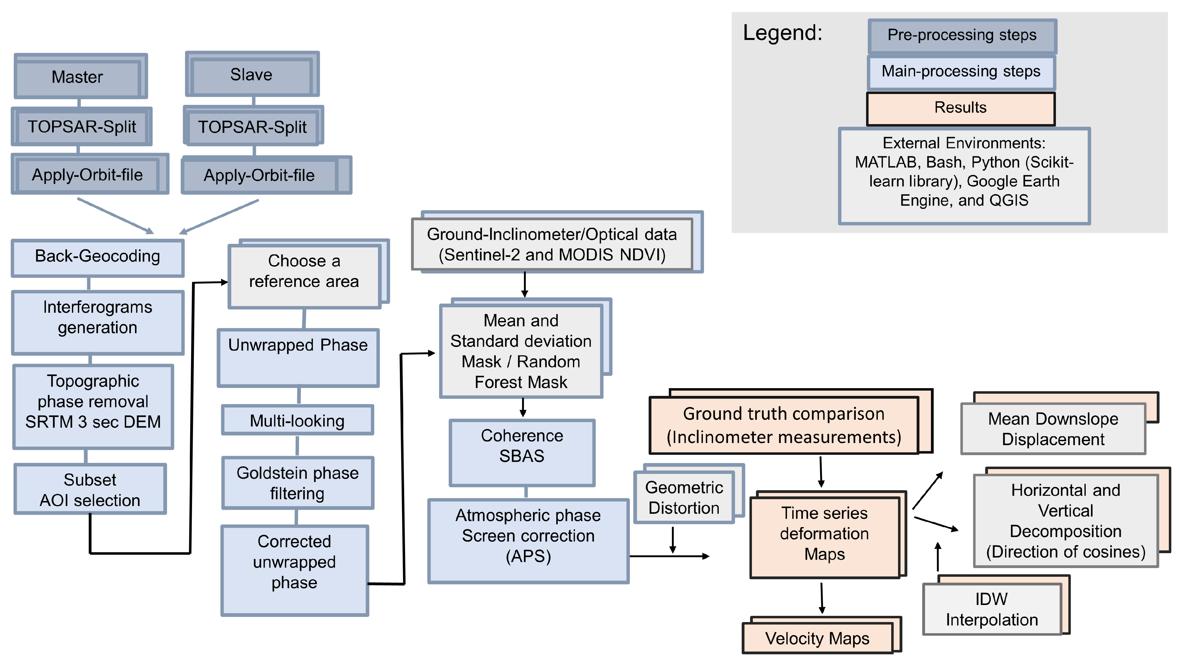
2.3. InSAR Dataset and Methods

Recently, multi-temporal InSAR (MT-InSAR) methods have been applied more widely than the classical differential InSAR (DInSAR) technique for the detection of slow-moving long-term displacement [24,25]. MT-InSAR analysis was conducted by using a satellite radar sensor from Sentinel-1 (S-1) (C-band wavelength, 5.6 cm), with a high spatial resolution of $5\times 20$ and 12-day revisit time over Japan, which was operated by the European Space Agency (ESA) and acquired wide-swath interferometric terrain observations with the Progressive Scan synthetic aperture radar mode. Single-look complex (SLC) images of 138 scenes along the ascending track and 140 scenes along the descending track were used. The phase was unwrapped by using the minimum-cost flow function (SNAPHU; [26]). Before initiating the small baseline subset (SBAS) approach [27], a stack of multi-look interferograms (with 8 looks in range and 2 looks in azimuth) was prepared with the consideration of the temporal period of the baseline analysis (from May 2016 to July 2021) by using the open-source GMTSAR software [28]; 417 and 422 interferograms were created with the same master dates for the ascending and descending tracks, respectively, which had a maximum baseline of 45 days and perpendicular baseline of less than 130 m. Ascending and descending measurements were referenced to the same pattern belonging to stable, low-relief morphology and low-vegetation-activity pixels [29]. In addition, tropospheric phase-delay effects were mitigated through the adoption of the common point stacking method [30]. One essential step in this process is the removal of low-coherence pixels [31] prior to the coherence-based CB-SBAS approach and during phase unwrapping (Figure 7); therefore, we examined two methods for removing such pixels from our InSAR analysis. The conventional method is based on calculating the means and standard deviations of coherence maps, and then masking out a random threshold coherence value that is similar or equal to the mean of this coherence value. Meanwhile, the proposed method uses a type of supervised machine learning, an RF model, to delineate the exact low-coherence pixels to be masked out. These steps can be used to assess the ground displacement related to distributed targets on the ground with moderate to high coherence, as illustrated in Figure 7.

2.4. Auxiliary Remote Sensing Data

Optical images can be combined with the outputs of InSAR to provide more information about the dynamics of landslides, in addition to capturing damage through a comparison of the surroundings before and after a landslide’s occurrence and examining the source of the received radar signal to determine whether it is a deformation signal or a false alarm caused by vegetation [32,33]. We used two types of optical images with different temporal and spatial resolutions: those of Sentinel-2, with a 10 m spatial resolution and 5-day temporal resolution, and those of MODIS, which provides daily imaging by using a bidirectional reflectance distribution function (BRDF) with a spatial resolution of 500 m. The NDVI is a parameter used to measure healthy green vegetation signals.

$$NDVI=\frac{NIR-RED}{NIR+RED},$$

(1)

RED is the red visible channel of the electromagnetic spectrum, and NIR is the near-infrared light channel. The procedures for selecting cloud cover and deriving the NDVI from optical images were implemented in the Google Earth Engine, and we collected MODIS time-series data for more than 6000 points over Otoyo Town to clearly capture the inverse linear relation between the NDVI and interferometric coherence. To perform this analysis, we developed Matlab and bash scripts, which began by removing the outliers from the MODIS NDVI data, followed by down-sampling of the MODIS NDVI time series to match the temporal resolution of the interferometric coherence time series (12 days), and then we observed the linear correlation ratio between the two independent curves (Figure 7).

2.5. Application of Supervised Machine Learning to Mitigate Decorrelation

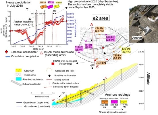
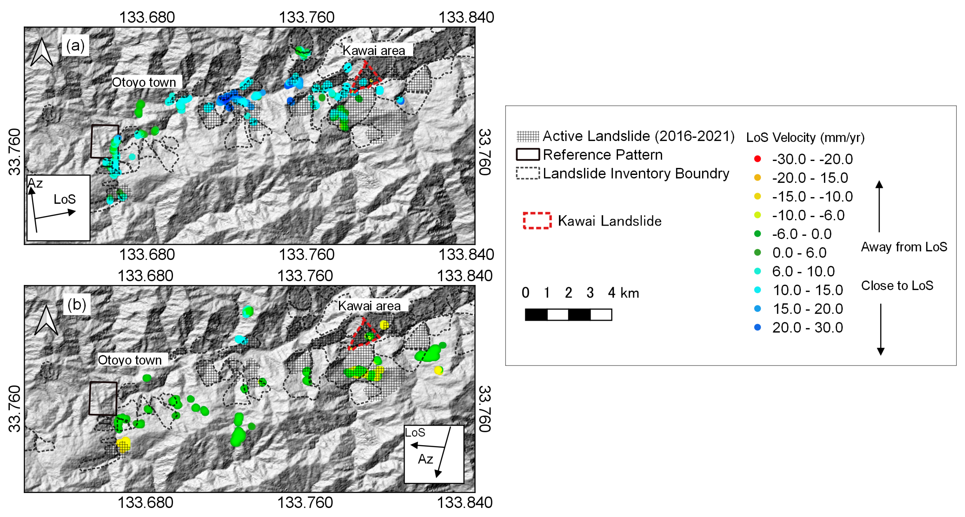
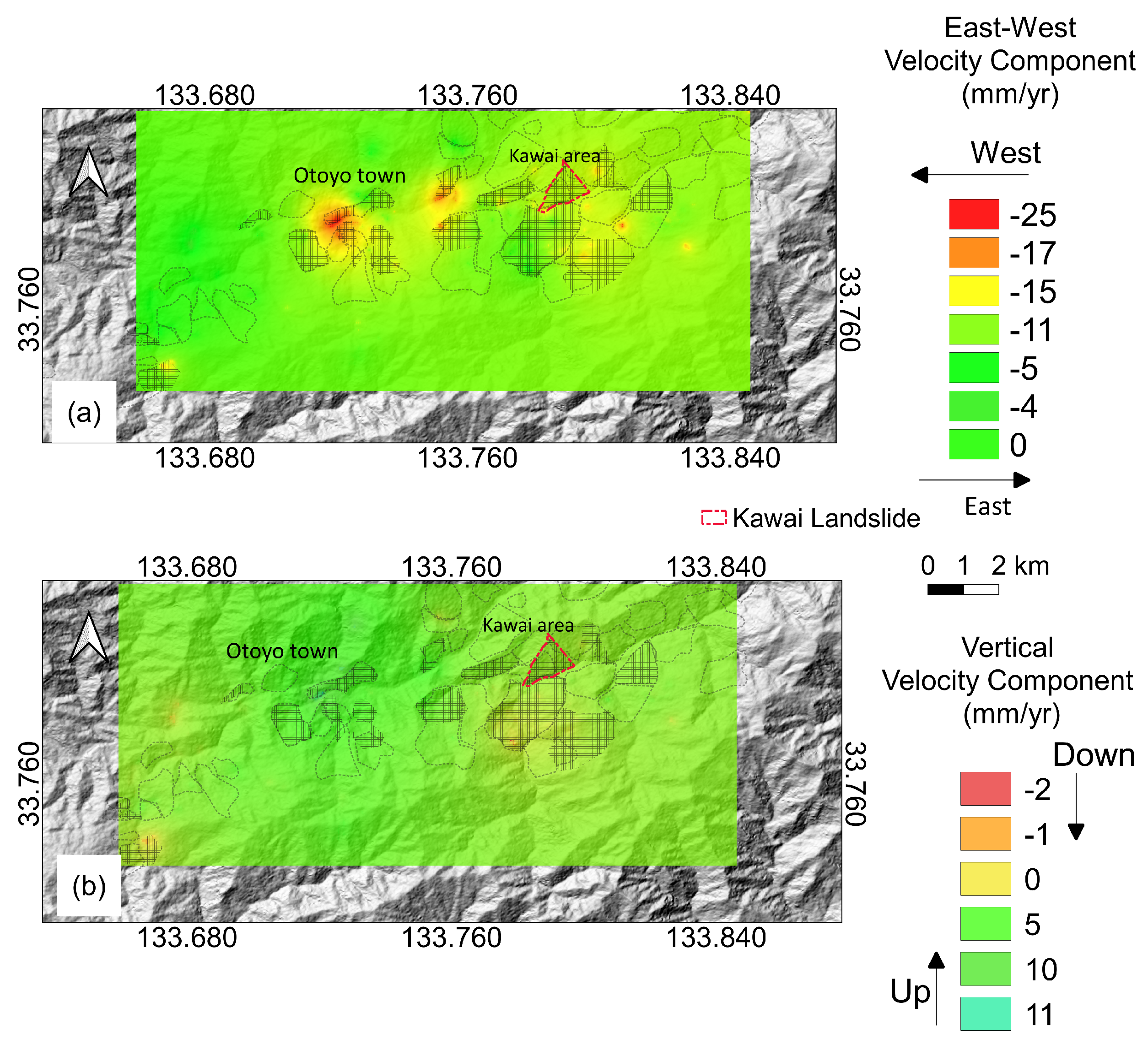
One key processing step in the selection of a suitable interferometric coherence threshold is obtaining the correct value for masking the low-coherence pixels related to water, high fractional canopy cover, and dense forests. This step can be challenging in regions covered with moderate-density or high-density vegetation, and applying the coherence mask to a large volume of data without removing any informative pixels related to slow-moving landslides is a further challenge. The landslide area includes three types of land cover: urban, field, and forest. Therefore, the discrimination of decorrelated pixels from noise across a large amount of data is challenging. Generally, supervised machine learning and, specifically, RF can classify and identify important features despite large volumes of data [34], and thus, we trained 345 points according to the inclinometer measurements, interferometric coherence, Sentinel-2, and MODIS NDVI data by using the RF model. The Sentinel-1 radar signal is readily scattered by dense vegetation, resulting in signal decorrelation; for this reason, we used the Sentinel-2 NDVI with a threshold value of 0.5 to avoid including decorrelated pixels related to dense forest locations [35]. The mean interferometric coherence threshold was set to 0.1 and was later discriminated by using the Sentinel-2 NDVI feature [36]. We began by training our model on three features—optical data, radar remote sensing data, and ground-truth data—followed by the implementation of the RF model across the whole scene covering Otoyo Town (6000 points) to predict reliable pixels and create a suitable low-coherence mask.

3. Results

3.1. Coherence-Based SBAS Measurement Results

R-index maps of the ascending and descending tracks were provided to precisely provide the low-sensitivity (due to geometric distortion) and high-sensitivity regions [9,22] for further consideration in the InSAR analysis. After applying the CB-SBAS approach, we noted that some pixels had high-velocity values (moving away from or toward the LoS). Few pixels were assessed due to the presence of low-coherence pixels in many locations—particularly fields and forests—and, therefore, we interpolated the LoS velocity results by using the inverse-distance-weighted (IDW) method (with a power of 1, the condition of selecting a minimum of three points, and a 100 m radius) [37,38]. Thereafter, the combination of interpolated ascending and descending LoS velocities was used to calculate the 2D deformation field to derive the E–W and vertical velocity components. The directions of the cosines (N, E, and H) of the ascending (Asc) and descending (Des) LoS vectors were estimated from the azimuth and incidence angles. The estimated values of the LoS directional cosines $E_{Asc}$, $E_{Des}$, $H_{Asc}$, and $H_{Des}$ were 0.6, 0.5, 0.7, and 0.8, respectively. However, the north component was negligible due to the lower sensitivity of the displacement along the north–south direction [37]. The horizontal and vertical components determined the dominant direction of movement, which was observed to be almost fully along the slope, with no vertical motion. The horizontal component (translational component) was estimated in some regions of Otoyo Town, which showed a dominant movement towards the west at a rate of approximately −21.4 mm/year. The InSAR pattern elucidated some active regions that intersected with active landslides that had already been observed in the ground-based inclinometer survey, which are annotated as black hashed polygons in Figure 5, while inactive areas were registered in the locations highlighted with black dotted polygons (historical landslides). Moreover, the LoS velocity was estimated with a mean of 13.19 mm/year and a standard deviation of 6.82 mm/year. The limited number of pixels distributed over the Kawai area prevented the application of 2D decomposition analysis and IDW interpolation (Figure 6). We also aimed to identify other active landslides that had not been detected through ground-based measurements due to the difficulty of access to these places or unintentional oversight, as local investigation is difficult and costly. Some locations had high movement rates in the ground-truth data that could not be detected via InSAR analysis, and vice versa; the reasons and limitations underlying this finding are discussed in Section 2.2 and Section 3. Ultimately, the integration of ground-based and remote-sensing techniques provides more detailed information about the nonlinear movements of landslides.

3.2. Comparison of the Ground-Anchor Tension Force, Inclinometer, and InSAR Time Series

We monitored the time-series displacement over 5 years, from 2016 to 2021, as well as the factors triggering landslides (primarily cumulative precipitation). Days with high precipitation were identified from on-site meteorological station measurements (located in the Kawai area at approximately 3.5 km from the time-series InSAR and inclinometer measurements). During this period, a trend in landslide motion was determined in the e2 region, the location of which is delineated in Figure 8; according to the two implemented tools, we observed the landslide displacement, and the only causes of deformation identified were cumulative precipitation and anchor instability. Ground-anchor tension surveys were performed three times in 2014, 2019, and 2020. Each tendon length of the three anchor heads was enumerated according to the back-calculation of the gradient-load-displacement curve for anchor elongation in 2014 [39]; as a consequence, the anchor lengths were designated as 14, 11, and 16 m rather than the original lengths of 34, 23, and 21 m, respectively. The conditions in the e2 area were stable until heavy precipitation events occurred in 2018 and 2019, when the residual tensile force dramatically increased to 736 kN. This tensile force was received from the plate and was restrained by the slip surface during the lift-off test in 2019 [40]. Therefore, the efficiency of the installed anchor was diminished, and it induced continued landslide movement. Based on the tension confirmation for all anchors, the theoretical elastic displacement was re-calculated, and the tendon lengths were adjusted for a second time in 2020 according to the lengths of 11, 10, and 12 m. After anchor maintenance, the landslide motion in the e2 region was terminated. Since 2020, the e2 region has shown stable behavior, with a clear but gradual decrease in the residual tensile force from a range of 593–481 to only 175 kN (Figure 3).

Although we could not assume any quantitative comparisons between the InSAR and inclinometer measurements [14], such a comparison may provide some beneficial information about the complex behavior of the slow-moving Kawai landslide to evaluate the accuracy of the InSAR results. For the inclinometer measurements, after the precipitation events in July 2018, the bearing capacities of the ground anchors in some locations exceeded their limits [23], and the inclinometer survey measured horizontal movement along the maximum slope in the direction of east to southeast. On the other hand, the tilting of the slide continued due to the increased load at the top of the slide caused by precipitation, leading to unequal stress and increased relative displacement (17.03 mm from 2016 to November 2019) on the surface of the anchor. After the ground anchors had been fixed through anchor elongation and increased bearing capacity, stable behavior was observed in the e2 area from the date of November 2020 to November 2021 ($\mathsf{\Delta }$t3 = 1.7 mm), as shown in Figure 9a. As we aimed to compare the LoS displacement with the ground-truth data, an accurate estimate of the true landslide motion along the downslope was needed, which was determined [41,42] as follows:

$${\mathit{D}}_{downslope}=\frac{D_{LoS}}{sin(\alpha -\beta )sin\left({\theta }_{inc}\right)sin\left({\theta }_{slp}\right)+cos\left({\theta }_{inc}\right)sin\left({\theta }_{slp}\right)},$$

(2)

where $\alpha$ is the heading direction or the S-1 azimuth flight direction, with positive values counterclockwise from the north; ${\theta }_{inc}$ is the S-1 incidence angle. The other parameters are related to the morphology of the landslide; $\beta$ is the azimuth or mean downslope direction of the landslide and ${\theta }_{slp}$ is the mean slope of the landslide. The InSAR and inclinometer measurement points found in the e2 area were separated by distances of 21.8, 40.5, and 78 m. Therefore, the displacement behavior described above was determined by using the InSAR time series from the ascending orbit moving toward the LoS. The high precipitation rate in July 2018 and anchor movement in May 2019 caused the mean downslope displacement to increase by $\mathsf{\Delta }$t1 = 11.8 mm and $\mathsf{\Delta }$t2 = 11.4 mm, respectively, while the anchor’s capacity was reached in 2020 and 2021 at $\mathsf{\Delta }$t3 = 1.1 mm, as shown in Figure 9a and

Table 1. Time increments related to the cumulative precipitation, borehole inclinometer, ground-anchor inefficiency, ground-anchor steady state, and InSAR mean downslope displacement data from June 2018 to September 2020 in the western channel of the Kawai landslide (e2 area).

$\mathsf{\Delta }$t1 (e2)	$\mathsf{\Delta }$t2 (e2)	$\mathsf{\Delta }$t3 (e2)
Heavy precipitation occurred in July 2018 (June–September)	Precipitation and anchor instability in June 2019 (April–July)	Precipitation in 2020 (May–September). The anchor has been completely stable since 2020

. Figure 4 illustrates the left loop of the Kawai landslide in the TC-1 area. The surface layer of this zone was saturated with groundwater, and landslide motion occurred in 2020 and 2021 (

Table 2. Time increments related to cumulative precipitation, borehole inclinometer, and InSAR mean downslope displacement data from June 2018 to August 2021 in the eastern channel of the Kawai landslide (TC-1 area).

$\mathsf{\Delta }$t1 (TC-1)	$\mathsf{\Delta }$t2 (TC-1)	$\mathsf{\Delta }$t3 and $\mathsf{\Delta }$t4 (TC-1)
Heavy precipitation in July 2018 (June–September)	Precipitation in June 2019 (April–July), inhabitants reported cracks	Precipitation from May to September 2020. From August 2020 to August 2021, the area was unstable

). There were also some fluctuations related to the seasonal behavior of the landslide due to the wet and slight drought of the soil [9]. For the landslide in the TC-1 area, inclinometer observations recorded a sudden increase in displacement beginning in December 2020 ($\mathsf{\Delta }$t1 = 3.54 mm/70 days), followed by another sharp increase of $\mathsf{\Delta }$t2 = 32.50 mm/ 10 months (as shown in Figure 9b). The distances between the InSAR displacement points and inclinometer boreholes in the TC-1 area were 28, 48, and 52 m, respectively.

The InSAR downslope time series exhibited high displacement values compared to those in the ground-truth data, especially in the e2 region, which is surrounded by forest. These downslope displacement values were obtained by using a conventional MSD mask (Figure 9a) to mask out low-coherence pixels (

Table 3. Borehole inclinometer and InSAR time series with the time increments from the cumulative precipitation comparison, together with the results obtained by using the conventional MSD mask and RF masks for comparison.

Time Increment of the e2 Area	$\mathsf{\Delta }$t1	$\mathsf{\Delta }$t2	$\mathsf{\Delta }$t3
Cumulative precipitation (mm)	2630	1070	3520
InSAR displacement [MSD mask] (mm)	11.8	11.4	1.1
InSAR displacement [RF mask] (mm)	3.5	10.5	0.7
Inclinometer Measurements	November 2016–June 2019		October 2019–November 2020
Displacement (mm)	15.46		1.7

); on the other hand, the InSAR downslope values approached the inclinometer values after the introduction of an RF mask to the CB-SBAS approach, as shown in Figure 9c and Table 3 and discussed in Section 2.3.

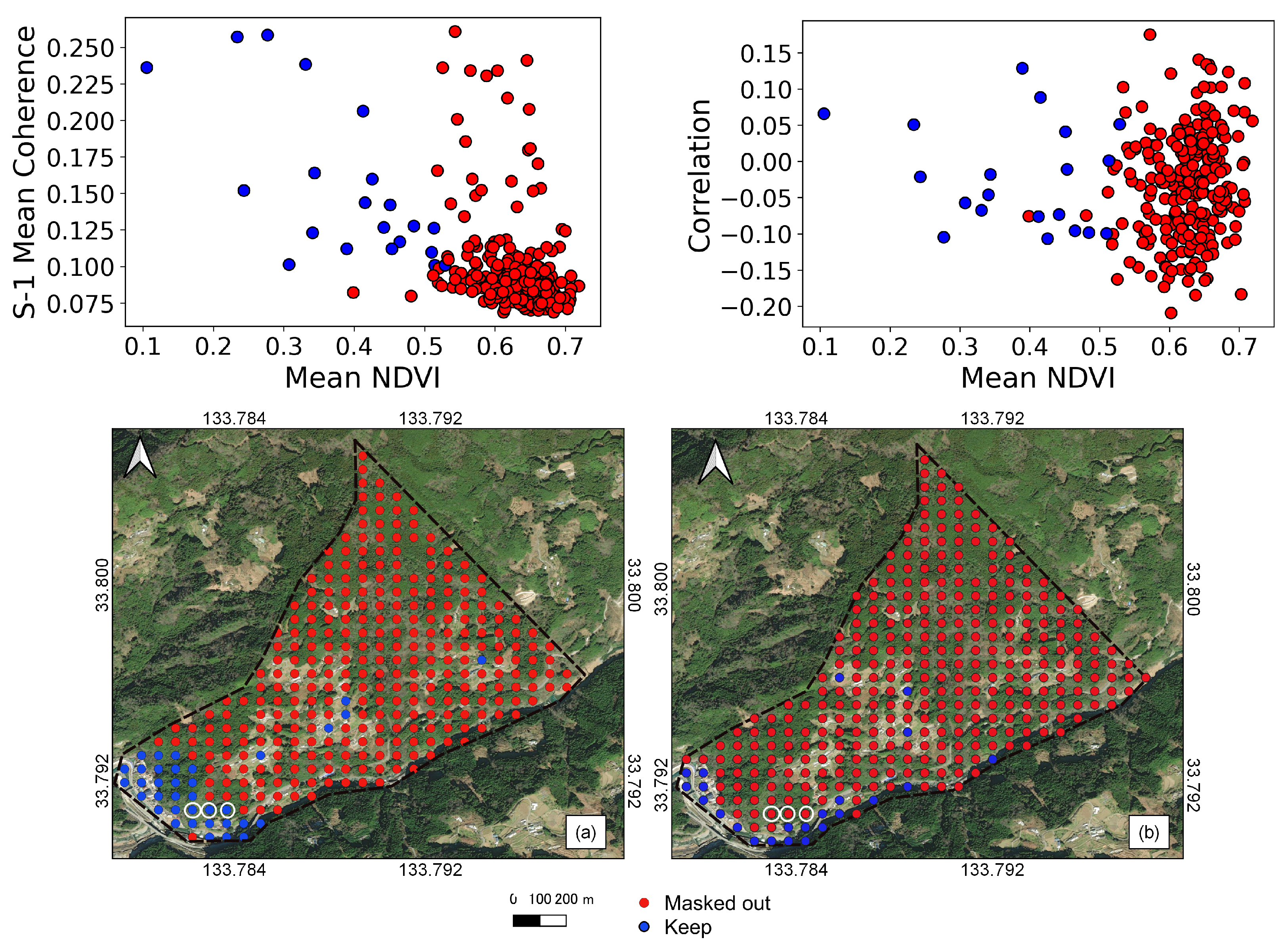
3.3. Random Forest Mask

The main objective of using an RF classification mask was to combine several features of pixel decorrelation indicators related to vegetation activity, including the mean values of the Sentinel-2 NDVI and MODIS NDVI and the correlation between the MODIS NDVI and S-1 interferometric coherence time series [17,43]. Although the MODIS NDVI and interferometric coherence time series had differences in spatial resolution, a good negative seasonal correlation was observed between them [16,17]. After calculating the exact values of the correlation between the NDVI from MODIS and the interferometric coherence over Otoyo Town (6948 points) ranging between −0.2 and 0.15, we observed that some pixels had a clear decrease in their coherence values with an increase in the NDVI during the summer season from June to October (the rainy season in Japan), whereas the interferometric values were high from November to April [16]. However, some deviations occurred in this relation, indicating displacement due to cumulative precipitation or ground-anchor movement. In these cases, an abrupt change in interferometric coherence values occurred that was unrelated to the behavior of the seasonal vegetation activity, representing damage (Figure 10a). This abrupt change led to inversely negative correlation values; such pixels may be included in further analyses or excluded with the low-coherence mask (expressed with blue dots). In contrast, pixels with high mean S-2 NDVI values and low S-1 mean coherence, which also showed strong negative correlations between the MODIS NDVI and S-1 interferometric coherence (lower than −0.1), were masked out, as shown in Figure 10b,c, and they are highlighted with red dots.

The RF was implemented by using the Python scikit-learn package [44]. The configuration parameters for RF classification for training were set to 80% of the low-coherence mask for the Kawai landslide, as these configuration parameters were considered the most important and reliable features of the model. The classification options had to be selected carefully, as they could affect the accuracy of the model; (1) the split criteria for the model were based on the minimization of the mean absolute error, (2) the number of estimators that comprised a forest was set to 100, (3) the function selected to assess the quality of the split was Gini, and (4) the random state responsible for input sample randomness was 10 [43,45]. Validation of the classification results could be conducted by extracting matrices with a confusion matrix [34], and our RF had an overall accuracy of 0.94. The training data were used to predict all data outside the test cells surrounding Otoyo Town, which included 6948 cells. Figure 11 shows the pixels that may have suffered decorrelation as a result of vegetation growth, with the forest pixels highlighted in white. Although this region was previously confirmed as stable based on ground observations, the RF included the white-highlighted pixels in the mask. Moreover, after the application of RF and the subsequent unwrapping process and CB-SBAS analysis (Figure 7), a lower-weighted RMS value with an average of 0.68 mm was observed from the uncertainty of the CB-SBAS linear regression (Figure 12), which provided a more accurate estimate of the downslope displacement from 58 to 23 mm (Figure 9a,c). In addition, the standard deviation from the estimation of the InSAR deformation rate across the whole of Otoyo Town after applying the RF model (4.9 mm/year) was generally lower than that obtained with the conventional method (6.8 mm/year).

4. Discussion

Landslide behavior cannot be monitored by using only LoS displacement due to the morphology of hill slopes, as a landslide’s displacement may be greater than a satellite’s spatial resolution. Consequently, in situ monitoring technologies, such as inclinometer surveys, are used to confirm and evaluate trends of landslide movement detected in satellite-based data. The accuracy of InSAR results related to landslide displacement depends on the location of the landslide along the LoS, the aspect and slope angle, and the vegetation cover. Inclinometer observations provide actual horizontal movement data along the slope direction and can be used to assess the limitations of the S-1 LoS by capturing motion in its blind zones. However, the InSAR velocity components across the whole of Otoyo Town successfully detected ten active landslides out of fifteen landslides. Focusing on the Kawai landslide, we found that only the Sentinel-1 descending track captured the slow downslope landslide movement in the TC-1 region, while the ascending track did not, as the TC-1 landslide motion was sub-parallel (N140${}^{\circ }$: 140${}^{\circ }$ measured clockwise from the north) to the azimuth of the S-1 ascending track [14]. We must also consider the limitation of the InSAR displacement results, which can measure only one component of displacement along the LoS, whereas an inclinometer measures the actual displacement along the maximum slope direction (as presented in Table 3 after applying the RF mask) [6,14]. In addition, a borehole inclinometer registers displacement after referring to a stable surface under a sliding surface, while the InSAR method measures displacement according to the LoS direction by referring to a stable pattern located at the surface [2]. We propose two reasons for this landslide movement—cumulative precipitation and ground anchors exceeding their capacity—which increased shear stress, leading to increased displacement. These landslide motions and the associated steady-state conditions were confirmed by using borehole inclinometer data, which clearly emphasized the accuracy of the space-borne SAR observations. Our research clearly shows the displacement and steady states of the Kawai landslide before and after the elongation of the ground-anchor tendons. The mean downslope displacement indicating the slow-moving landslide was captured and evaluated by using the CB-SBAS approach, and no discrepancy was found between the displacement measurements derived from the ground-based inclinometer and the tensile force obtained from anchor readings. This displacement calculation was improved by the application of the RF mask in order to remove low-coherence pixels related to canopy activity.

5. Conclusions

According to our analysis, the slow ground movement of landslides in Otoyo Town could be observed by using ground borehole inclinometers and the S-1 C-band radar satellite sensor. Consistent correlations among time-series measurements from ground inclinometers, ground-anchor pressures, cumulative precipitation, and S-1 downslope displacement were presented. The ground-anchor instability and steady state could be evaluated by using the CB-SBAS approach. Finally, RF, a supervised machine learning tool, could be applied as a low-coherence mask to mitigate the decorrelation effect associated with vegetation activity. In the future, we will combine the two integrated methods by converting the InSAR data to check for continuous analysis, and we will assess the reliability through a comparison of the InSAR outputs with borehole inclinometer records. This method can reduce the expenses involved in drilling new boreholes and minimize false peaks or outliers in the time-series displacement data obtained with each technique [7]. Moreover, installing corner reflectors in landslide regions covered with a high active canopy and lacking strong reflectors (such as buildings) will allow more stable InSAR phases to be reached, thus facilitating comparisons of ground- and satellite-based displacement information [9,46]. In addition, multi-sensor analysis can be conducted by using L-band satellite sensors, such as ALOS-4 or NISAR, and the new satellite sensors that will be launched in the near future have improved performance and functionality, thus supporting more accurate and precise observations of slow landslide movements, especially in vegetated areas.

References

1. Sasahara, K.; Ikeda, T.; Iwai, Y.; Kakuta, K.; Kanazawa, A.; Gonda, Y.; Saitou, Y.; Shuin, Y.; Tagata, S.; Fujita, M.; et al. Sediment disasters in Shikoku region in July, 2018. Int. J. Eros. Control Eng. 2019, 71, 43–53. [Google Scholar]
2. Bru, G.; Escayo, J.; Fernández, J.; Mallorqui, J.J.; Iglesias, R.; Sansosti, E.; Abajo, T.; Morales, A. Suitability Assessment of X-Band Satellite SAR Data for Geotechnical Monitoring of Site Scale Slow Moving Landslides. Remote Sens. 2018, 10, 936. [Google Scholar] [CrossRef] [Green Version]
3. Cook, M.E.; Brook, M.S.; Hamling, I.J.; Cave, M.; Tunnicliffe, J.F.; Holley, R.; Alama, D.J. Engineering geomorphological and InSAR investigation of an urban landslide, Gisborne, New Zealand. Landslides 2022, 19, 2423–2437. [Google Scholar] [CrossRef]
4. Campbell, K.E.J.; Ruffell, A.; Pringle, J.; Hughes, D.; Taylor, S.; Devlin, B. Bridge Foundation River Scour and Infill Characterisation Using Water-Penetrating Radar. Remote Sens. 2021, 13, 2542. [Google Scholar] [CrossRef]
5. Medhat, N.I.; Atya, M.; Ragab, E.A.; El-Kenawy, A.A.; Zaher, M.A.; Pringle, J.K. Geophysical site assessment of an active urban development site, southeastern suburb of Cairo, Egypt. Q. J. Eng. Geol. Hydrogeol. 2021, 54, qjegh2018-151. [Google Scholar] [CrossRef]
6. Tofani, V.; Raspini, F.; Catani, F.; Casagli, N. Persistent scatterer interferometry (psi) technique for landslide characterization and monitoring. Remote Sens. 2013, 5, 1045–1065. [Google Scholar] [CrossRef] [Green Version]
7. Bordoni, M.; Vivaldi, V.; Bonì, R.; Spanò, S.; Tararbra, M.; Lanteri, L.; Parnigoni, M.; Grossi, A.; Figini, S.; Meisina, C. A methodology for the analysis of continuous time-series of automatic inclinometers for slow-moving landslides monitoring in Piemonte region, northern Italy. Nat. Hazards 2022. [Google Scholar] [CrossRef]
8. Fujiwara, Y.; Sakai, T. A Study of a Lift-Off Test Method for Ground Anchors. J. JSCE 2016, 4, 106–117. [Google Scholar] [CrossRef]
9. Kelevitz, K.; Novellino, A.; Watlet, A.; Boyd, J.; Whiteley, J.; Chambers, J.; Jordan, C.; Wright, T.; Hooper, A.; Biggs, J. Ground and Satellite-Based Methods of Measuring Deformation at a UK Landslide Observatory: Comparison and Integration. Remote Sens. 2022, 14, 2836. [Google Scholar] [CrossRef]
10. Ao, M.; Zhang, L.; Dong, Y.; Su, L.; Shi, X.; Balz, T.; Liao, M. Characterizing the evolution life cycle of the Sunkoshi landslide in Nepal with multi-source SAR data. Sci. Rep. 2020, 10, 1–12. [Google Scholar] [CrossRef]
11. Hamama, I.; Yamamoto, M.-Y.; ElGabry, M.N.; Medhat, N.I.; Elbehiri, H.S.; Othman, A.S.; Abdelazim, M.; Lethy, A.; El-hady, S.M.; Hussein, H. Investigation of near-surface chemical explosions effects using seismo-acoustic and synthetic aperture radar analyses. J. Acoust. Soc. Am. 2022, 151, 1575–1592. [Google Scholar] [CrossRef] [PubMed]
12. Zhang, T.; Shen, W.B.; Wu, W.; Zhang, B.; Pan, Y. Recent surface deformation in the Tianjin area revealed by Sentinel-1A data. Remote Sens. 2019, 11, 130. [Google Scholar] [CrossRef] [Green Version]
13. Darwish, N.; Kaiser, M.; Koch, M.; Gaber, A. Assessing the accuracy of alos/palsar-2 and sentinel-1 radar images in estimating the land subsidence of coastal areas: A case study in alexandria city, egypt. Remote Sens. 2021, 13, 1838. [Google Scholar] [CrossRef]
14. Wasowski, J.; Pisano, L. Long-term InSAR, borehole inclinometer, and rainfall records provide insight into the mechanism and activity patterns of an extremely slow urbanized landslide. Landslides 2020, 17, 445–457. [Google Scholar] [CrossRef]
15. Novellino, A.; Cesarano, M.; Cappelletti, P.; Di Martire, D.; Di Napoli, M.; Ramondini, M.; Sowter, A.; Calcaterra, D. Slow-moving landslide risk assessment combining Machine Learning and InSAR techniques. Catena 2021, 203, 105317. [Google Scholar] [CrossRef]
16. Xia, Z.; Motagh, M.; Li, T.; Roessner, S. The June 2020 Aniangzhai landslide in Sichuan Province, Southwest China: Slope instability analysis from radar and optical satellite remote sensing data. Landslides 2022, 19, 313–329. [Google Scholar] [CrossRef]
17. Jacquemart, M.; Tiampo, K. Leveraging time series analysis of radar coherence and normalized difference vegetation index ratios to characterize pre-failure activity of the Mud Creek landslide, California. Nat. Hazards Earth Syst. Sci. 2021, 21, 629–642. [Google Scholar] [CrossRef]
18. Bai, Z.; Fang, S.; Gao, J.; Zhang, Y.; Jin, G.; Wang, S.; Zhu, Y.; Xu, J. Could Vegetation Index be Derive from Synthetic Aperture Radar?—The Linear Relationship between Interferometric Coherence and NDVI. Sci. Rep. 2020, 10, 6749. [Google Scholar] [CrossRef] [Green Version]
19. Jacob, A.W.; Notarnicola, C.; Suresh, G.; Antropov, O.; Ge, S.; Praks, J.; Ban, Y.; Pottier, E.; Mallorqui Franquet, J.J.; Duro, J.; et al. Sentinel-1 InSAR Coherence for Land Cover Mapping: A Comparison of Multiple Feature-Based Classifiers. IEEE J. Sel. Top. Appl. Earth Obs. Remote Sens. 2020, 13, 535–552. [Google Scholar] [CrossRef] [Green Version]
20. Confuorto, P.; Medici, C.; Bianchini, S.; Del Soldato, M.; Rosi, A.; Segoni, S.; Casagli, N. Machine Learning for Defining the Probability of Sentinel-1 Based Deformation Trend Changes Occurrence. Remote Sens. 2022, 14, 1748. [Google Scholar] [CrossRef]
21. Sato, G.; Ozaki, T.; Yokoyama, O.; Wakai, A.; Hayashi, K.; Yamasaki, T.; Tosa, S.; Mayumi, T.; Kimura, T. New approach for the extraction method of landslide-prone slopes using geomorphological analysis: Feasibility study in the Shikoku mountains, Japan. J. Disaster Res. 2021, 16, 618–625. [Google Scholar] [CrossRef]
22. Notti, D.; Herrera, G.; Bianchini, S.; Meisina, C.; García-Davalillo, J.C.; Zucca, F. A methodology for improving landslide PSI data analysis. Int. J. Remote Sens. 2014, 35, 2186–2214. [Google Scholar] [CrossRef]
23. Fang, G.W.; Zhu, Y.P.; Ye, S.H.; Huang, A.P. Analysis of force and displacement of anchor systems under the non-limit active state. Sci. Rep. 2022, 12, 1306. [Google Scholar] [CrossRef]
24. Medhat, N.I.; Yamamoto, M.-Y.; Tolomei, C.; Harbi, A.; Maouche, S. Multi-temporal InSAR analysis to monitor landslides using the small baseline subset (SBAS) approach in the Mila Basin, Algeria. Terra Nova 2022, 34, 407–423. [Google Scholar] [CrossRef]
25. Pawluszek-Filipiak, K.; Borkowski, A. Integration of DInSAR and SBAS techniques to determine mining-related deformations using Sentinel-1 data: The case study of rydultowy mine in Poland. Remote Sens. 2020, 12, 242. [Google Scholar] [CrossRef] [Green Version]
26. Chen, C.; Zebker, H. Phase unwrapping for large SAR interferograms: Statistical segmentation and generalized network models. IEEE Trans. Geosci. Remote Sens. 2002, 40, 1709–1719. [Google Scholar] [CrossRef] [Green Version]
27. Berardino, P.; Fornaro, G.; Lanari, R.; Sansosti, E. A new algorithm for surface deformation monitoring based on small baseline differential SAR interferograms. IEEE Trans. Geosci. Remote Sens. 2002, 40, 2375–2383. [Google Scholar] [CrossRef] [Green Version]
28. Sandwell, D.; Mellors, R.; Tong, X.; Wei, M.; Wessel, P. Open radar interferometry software for mapping surface Deformation. Eos Trans. Am. Geophys. Union 2011, 92, 234. [Google Scholar] [CrossRef] [Green Version]
29. Cianflone, G.; Tolomei, C.; Brunori, C.A.; Monna, S.; Dominici, R. Landslides and subsidence assessment in the Crati Valley (Southern Italy) using insar data. Geosciences 2018, 8, 67. [Google Scholar] [CrossRef] [Green Version]
30. Tymofyeyeva, E.; Fialko, Y. Mitigation of atmospheric phase delays in InSAR data, with application to the eastern California shear zone. J. Geophys. Res. Solid Earth 2015, 120, 5952–5963. [Google Scholar] [CrossRef]
31. Tong, X.; Schmidt, D. Active movement of the Cascade landslide complex in Washington from a coherence-based InSAR time series method. Remote Sens. Environ. 2016, 186, 405–415. [Google Scholar] [CrossRef]
32. Liang, J.; Dong, J.; Zhang, S.; Zhao, C.; Liu, B.; Yang, L.; Yan, S.; Ma, X. Discussion on InSAR Identification Effectivity of Potential Landslides and Factors That Influence the Effectivity. Remote Sens. 2022, 14, 1952. [Google Scholar] [CrossRef]
33. Morishita, Y. Nationwide urban ground deformation monitoring in Japan using Sentinel-1 LiCSAR products and LiCSBAS. Prog. Earth Planet. Sci. 2021, 8, 6. [Google Scholar] [CrossRef]
34. Mirmazloumi, S.M.; Gambin, A.F.; Palam, R.; Crosetto, M. Supervised Machine Learning Algorithms for Ground Motion Time Series Supervised Machine Learning Algorithms for Ground Motion Time Series Classification from InSAR Data. Remote Sens. 2022, 14, 3821. [Google Scholar] [CrossRef]
35. Karlsen, S.R.; Stendardi, L.; Tømmervik, H.; Nilsen, L.; Arntzen, I.; Cooper, E.J. Time-series of cloud-free sentinel-2 ndvi data used in mapping the onset of growth of central spitsbergen, svalbard. Remote Sens. 2021, 13, 3031. [Google Scholar] [CrossRef]
36. Karimzadeh, S.; Matsuoka, M.; Miyajima, M.; Adriano, B.; Fallahi, A.; Karashi, J. Sequential SAR coherence method for the monitoring of buildings in Sarpole-Zahab, Iran. Remote Sens. 2018, 10, 1255. [Google Scholar] [CrossRef] [Green Version]
37. Béjar-Pizarro, M.; Notti, D.; Mateos, R.M.; Ezquerro, P.; Centolanza, G.; Herrera, G.; Bru, G.; Sanabria, M.; Solari, L.; Duro, J.; et al. Mapping Vulnerable Urban Areas Affected by Slow-Moving Landslides Using Sentinel-1 InSAR Data. Remote Sens. 2017, 9, 876. [Google Scholar] [CrossRef] [Green Version]
38. Bayramov, E.; Buchroithner, M.; Kada, M.; Zhuniskenov, Y. Quantitative assessment of vertical and horizontal deformations derived by 3d and 2d decompositions of insar line-of-sight measurements to supplement industry surveillance programs in the tengiz oilfield (Kazakhstan). Remote Sens. 2021, 13, 2579. [Google Scholar] [CrossRef]
39. Japan Anchor Association. Inspection and Maintenance Manual for Ground Anchors; Japan Anchor Association: Tokyo, Japan, 2015. [Google Scholar]
40. Hamasaki, T.; Kasama, K.; Maeda, Y. Deterioration model of ground anchor for slope stability assessment. Jpn. Geotech. Soc. Spec. Publ. 2015, 2, 2461–2464. [Google Scholar] [CrossRef] [Green Version]
41. Liu, L.; Millar, C.I.; Westfall, R.D.; Zebker, H.A. Surface motion of active rock glaciers in the Sierra Nevada, California, USA: Inventory and a case study using InSAR. Cryosphere 2013, 7, 1109–1119. [Google Scholar] [CrossRef] [Green Version]
42. Handwerger, A.L.; Fielding, E.J.; Sangha, S.S.; Bekaert, D.P. Landslide Sensitivity and Response to Precipitation Changes in Wet and Dry Climates. Geophys. Res. Lett. 2022, 49, e2022GL099499. [Google Scholar] [CrossRef] [PubMed]
43. Burrows, K.; Milledge, D.; Walters, R.; Bellugi, D. Improved rapid landslide detection from integration of empirical models and satellite radar. Nat. Hazards Earth Syst. Sci. 2021, 765, 1–34. [Google Scholar]
44. Pedregosa, F.; Varoquaux, G.; Gramfort, A.; Michel, V.; Thirion, B.; Grisel, O.; Blondel, M.; Prettenhofer, P.; Weiss, R.; Dubourg, V.; et al. Scikit-learn: Machine Learning in Python. J. Mach. Learn. Res. 2011, 12, 2825–2830. [Google Scholar]
45. Ziegler, A.; König, I.R. Mining data with random forests: Current options for real-world applications. WIREs Data Min. Knowl. Discov. 2014, 4, 55–63. [Google Scholar] [CrossRef]
46. Bovenga, F.; Pasquariello, G.; Pellicani, R.; Refice, A.; Spilotro, G. Landslide monitoring for risk mitigation by using corner reflector and satellite SAR interferometry: The large landslide of Carlantino (Italy). Catena 2017, 151, 49–62. [Google Scholar] [CrossRef]
Figure 1. Map of Kochi Prefecture in Japan, including the study area (a), the location of Otoyo Town (b). The yellow and red rectangles represent the ascending and descending frames from Sentinel-1, respectively.
Remotesensing 15 00441 g001
Figure 2. Map of the active landslide in Otoyo Town (a), the Kawai landslide (b), and the channels of the Kawai landslide; e2 area (c) and TC-1 (d). The two channels of the Kawai landslide were monitored by using anchor pressure and borehole inclinometer surveys (presented in Figure 3 and Figure 4).
Remotesensing 15 00441 g002
Figure 3. Anchor tension distribution map and the locations of anchors in Otoyo Town associated with the Kawai landslide and e2 area. The cross-section A–A’ shows the geological and geomorphological setting, borehole inclinometer locations, and subsurface tendons of the anchors. The shear stress gradually decreased after anchor maintenance in 2020, and anchors are indicated by in pink and yellow colors.
Remotesensing 15 00441 g003
Figure 4. Diagram showing landslide movement in the TC-1 area corresponding to the surface damage caused to homes and infrastructure (a,b), ground truth observations (c,d), as well as water springs, with a geological cross-section B–B’ indicating the locations of the inclinometer boreholes that provided data on depth to the sliding surface and water springs.
Remotesensing 15 00441 g004
Figure 5. Sentinel-1 LoS velocity maps in Otoyo Town. The results of the LoS velocity analysis of the S-1 ascending track: (a) Blue regions indicate movement toward the LoS. The LoS velocity analysis results for the S-1 descending track: (b) Red regions represent movement away from the LoS. All LoS points are referenced against a stable, unvegetated, and low-relief pattern annotated with a black rectangle. The hashed regions represent active landslides, which were assessed by using inclinometer measurements from 2016 to 2021.
Remotesensing 15 00441 g005
Figure 6. Horizontal and vertical components after inverted distance-weighted interpolation and decomposition of both the ascending and descending LoS velocity values. Horizontal component: (a) active landslide locations moving towards the west along the slope direction; vertical component: (b) minor vertical movement in the downward direction.
Remotesensing 15 00441 g006
Figure 7. Flowchart of the processing steps implemented in this study.
Remotesensing 15 00441 g007
Figure 8. Detailed layout of the Kawai area showing the InSAR and ground inclinometer measurements. The diamond symbols are ground inclinometer readings, whereby the horizontal movement and tilting of the sliding surface during the Kawai landslide were measured along the direction of the slope. The colored triangular symbols indicate the velocities obtained from the S-1 ascending track (positive values captured motion toward the LoS), while the S-1 velocity values of the descending track (negative values indicate the same movement away from the LoS) are shown as squares.
Remotesensing 15 00441 g008
Figure 9. Trend comparison of the time series of the mean downslope displacement and horizontal inclinometer measurements along the maximum slope (e2 and TC-1). (a) This comparison defines the InSAR mean downslope displacement of the S-1 ascending track and inclinometer displacement increments in the e2 region over three periods: Δ t 1 , Δ t 2 , and Δ t 3 . The first two increments, Δ t 1 and Δ t 2 , show ground deformation in the presence of ground anchors, while Δ t 3 represents stable readings of the InSAR and borehole inclinometer time series due to anchor elongation, despite the large increments in cumulative precipitation. (b) Comparison between the InSAR mean downslope movement based on the S-1 descending track and the inclinometer observations in the TC-1 area in four periods: Δ t 1 , Δ t 2 , Δ t 3 , and Δ t 4 , with the fourth period representing high mean downslope displacement increments driven by high cumulative precipitation in 2020 and 2021, when groundwater springs were observed on the surface. The inclinometer locations in the e2 and TC-1 areas are illustrated in Figure 3, Figure 4 and Figure 8. (c) Mean downslope time-series displacement after the application of the RF mask in the e2 region; there is a correlation between the cumulative displacement from the ground inclinometer and the InSAR mean downslope time series that is stronger than the correlations presented in (a).
Remotesensing 15 00441 g009
Figure 10. The inversely linear correlation relation between the S-1 interferometric coherence and MODIS NDVI time series. (a) An example of a pixel to be excluded from an RF mask, as it may be related to ground motion (S-1 interferometric coherence values decrease with the decline in the MODIS NDVI curve). (b,c) Example of pixels to be masked out.
Remotesensing 15 00441 g010
Figure 11. New samples classified according to the split of the RF model; blue points refer to pixels included in the analysis, while red points are masked out. The features were the mean NDVI and S-1 mean coherence (a), and the mean NDVI and the correlation between the S1 coherence and the NDVI time series (b). Georeferencing of pixels took place before and after the application of the RF mask, where white-highlighted pixels represent forest regions; these pixels were excluded from the CB-SBAS analysis and show no sign of displacement in the ground survey observations.
Remotesensing 15 00441 g011
Figure 12. Comparison of the root mean square (RMS) before (a) and after the application of the RF mask (b) derived from the uncertainty estimate for the SBAS velocity from a linear regression. (c) The majority of the RMS values at active landslide boundaries (yellow hashed polygons) decreased by 0.3 mm in Otoyo Town (yellow dots), while a few points located in the stable zones (red dots) had increased RMS values after the application of the RF mask.
Remotesensing 15 00441 g012