Article

A New Method for the Rapid Determination of Fire Disturbance Events Using GEE and the VCT Algorithm—A Case Study in Southwestern and Northeastern China

1
Co-Innovation Center for Sustainable Forestry in Southern China, Nanjing Forestry University, Nanjing 210037, China
2
College of Forestry, Nanjing Forestry University, Nanjing 210037, China
*
Author to whom correspondence should be addressed.
Remote Sens. 2023, 15(2), 413; https://doi.org/10.3390/rs15020413
Submission received: 9 November 2022 / Revised: 5 January 2023 / Accepted: 9 January 2023 / Published: 10 January 2023

Abstract

:
Forest fires are major disturbances in forest ecosystems. The rapid detection of the spatial and temporal characteristics of fires is essential for formulating targeted post-fire vegetation restoration measures and assessing fire-induced carbon emissions. We propose an accurate and efficient framework for extracting the spatiotemporal characteristics of fires using vegetation change tracker (VCT) products and the Google Earth Engine (GEE) platform. The VCT was used to extract areas of persistent forest and forest disturbance patches from Landsat images of Xichang and Muli, Liangshan prefecture, Sichuan province in southwestern China and Huma, Heilongjiang province, in northeastern China. All available Landsat images in the GEE platform in a year were normalized using the VCT-derived persisting forest mask to derive three standardized vegetation indices (normalized burn ratio (NBRr), normalized difference moisture index (NDMIr), and normalized difference vegetation index (NDVIr)). Historical forest disturbance events in Xichang were used to train two decision trees using the C4.5 data mining tool. The differenced NBRr, NDMIr, and NDVIr (dNBRr, dNDMIr, and dNDVIr) were obtained by calculating the difference in the index values between two temporally adjacent images. The occurrence time of disturbance events were extracted using the thresholds identified by decision tree 1. The use of all available images in GEE narrowed the disturbance occurrence time down to 16 days. This period was extended if images were not available or had cloud cover. Fire disturbances were distinguished from other disturbances by comparing the dNBRr, dNDMIr, and dNDVIr values with the thresholds identified by decision tree 2. The results showed that the proposed framework performed well in three study areas. The temporal accuracy for detecting disturbances in the three areas was 94.33%, 90.33%, and 89.67%, the classification accuracy of fire and non-fire disturbances was 85.33%, 89.67%, and 83.67%, and the Kappa coefficients were 0.71, 0.74, and 0.67, respectively. The proposed framework enables the efficient and rapid extraction of the spatiotemporal characteristics of forest fire disturbances using frequent Landsat time-series data, GEE, and VCT products. The results can be used in forest fire disturbance databases and to implement targeted post-disturbance vegetation restoration practices.

1. Introduction

Forests provide more than 80% of the global above-ground biomass and are critical for terrestrial ecosystem carbon cycling [1,2]. They are subject to various disturbances [3,4,5], such as fire, logging, pests, and diseases [6]. The frequency and intensity of disturbances influence the forest ecosystems’ integrity and resilience. Forest fires are a frequent disturbance type and can cause extensive damage to forest ecosystems, in turn affecting people [7,8]. Therefore, monitoring and managing forest fires are required to ensure forest ecosystem health and the safety of forest-dependent people.
Traditional forest disturbance monitoring methods cannot meet today’s demand for high accuracy and timeliness of forest disturbance monitoring due to their high costs, high risk, long cycle time, and limited spatial accessibility [9]. Due to advances in remote sensing technology and computerized image processing and analysis algorithms, analyzing multi-temporal satellite remote sensing images provides a more convenient and timely method for forest change monitoring research [10,11,12]. In the early stage, disturbance identification methods using remote sensing data were generally based on the comparison of bi-temporal images or multitemporal images with relatively long time intervals [13]. Some low-intensity disturbance events could not be identified during the time interval. An increasing number of studies have used dense time series of remote sensing images to analyze forest changes [14,15] due to the greater availability and diversity of remote sensing data, such as Landsat and Sentinel [16] and automated analytical algorithms. Landsat images have a medium spatial resolution of 30 m, a temporal resolution of 16 days, and multispectral information, which is highly suitable for landscape-level forest disturbance analysis [17]. Several automated and reputable time-series analysis algorithms have been developed for forest disturbance monitoring using Landsat long time-series data, including the vegetation change tracker (VCT) [6], LandTrendr [18], continuous change detection and classification (CCDC) [19], and breaks for additive seasonal and trend (BFAST) [20]. The VCT algorithm has high efficiency, easy implementation, and high accuracy for identifying high-intensity disturbances, such as clearcuts and fire events. However, it is difficult to identify low-intensity disturbances and disturbances that recover quickly [6,14]. Additionally, the VCT does not provide attributes for the mapped disturbance events. Zhao et al. [21] performed attribution analysis of VCT-mapped disturbance events using a support vector machine (SVM) classifier; however, this method requires extensive ground-truth data of different disturbance events for classifier training and validation, and some parameters require substantial tuning [21]. Thus, a more efficient and easily implemented method is needed to overcome these deficiencies, especially for distinguishing fire-induced disturbance events from other disturbances.
The VCT algorithm is typically used with a Landsat time-series stack with intervals of 1 or 2 years. Disturbances occurring within this interval may have started to recover naturally or by anthropogenic influence [22,23], creating difficulties in forest disturbance type identification. If Landsat images with shorter time intervals are used to distinguish forest disturbance types, many remote sensing images are required, increasing the likelihood of images with high cloud cover. The images must be pre-processed to remove cloud contamination to enable the accurate identification of the disturbance type and disturbance time. The Google Earth Engine (GEE) platform has provided a convenient environment for forest fire identification and monitoring in recent years due to its massive remote sensing image datasets and powerful computing power. For example, GEE provides all available Landsat images for the last 40 years with a nominal time interval of 16 days, including TM, ETM+, and OLI. If two Landsat satellites are available, such as Landsat 7 and Landsat 8 or Landsat 8 and Landsat 9, the revisit cycle is shortened to 8 days. The GEE platform also provides surface reflectance (SR) images and a convenient tool for cloud masking [14], substantially reducing the pre-processing complexity and workload for a large number of remotely sensed images. Several studies related to forest disturbances have been conducted using the GEE platform. Bar et al. identified fire patches in India using supervised classification methods, such as classification and regression tree (CART), random forest (RF), and SVM on the GEE platform [24]. Li et al. extracted multiple forest disturbances, such as fire and deforestation, using the LandTrendr algorithm on the GEE platform [25]. Hua et al. used all available Landsat time-series image data in GEE to map forest disturbance and restoration events [14]. However, most of these studies that classified forest disturbance types required training samples in each scene to classify each image separately, substantially reducing the efficiency and preventing the ability to apply the method to other regions.
The selection of appropriate node characteristics is crucial in constructing decision tree rules with high generalization ability. Vegetation indices derived from satellite images are commonly used to identify forest disturbance and classify disturbance types [14,26,27]. This goal is typically achieved by obtaining the difference in SR of different wavelengths between images acquired before and after a forest disturbance [27,28]. Commonly used vegetation indices for forest disturbance analyses include the normalized burn ratio (NBR), normalized difference moisture index (NDMI), normalized difference vegetation index (NDVI), and tasseled cap transformation [18,29,30]. Among them, NBR is often used to extracting fire disturbance [22,31,32,33], NDMI can reflect the surface moisture content and is good for detecting forest harvesting [34], NDVI is widely used in vegetation-related studies [35]. However, the images may not be spectrally consistent due to different acquisition times, lowering the identification accuracy of disturbance events [36,37]. This inconsistency is one reason the decision rules obtained from samples of one image do not apply well to another image. Several studies have shown that the influence of image variability on the identification results can be mitigated by standardizing the vegetation indices [15,38,39]. Therefore, normalizing different vegetation indices created from images acquired at different times using different methods should improve the generalization ability of decision tree rules.
In China, the occurrence of forest disturbances is closely linked to human factors, local cultural customs, and production characteristics in different regions [25,40,41]. Different forest disturbances require different forest management and restoration measures to recover. The ability to distinguish different forest disturbance types rapidly and effectively enables the implementation of targeted preventive and management measures in a timely manner. The Liangshan Yi Autonomous Prefecture in Sichuan Province, China, is rich in forest resources, and the Daxinganling region in northeastern China experiences frequent fire events. Thus, these locations are suitable for validating our proposed framework for forest fire information extraction. The study of forest disturbance monitoring and identification can help forest managers improve their fire management practices and apply targeted post-fire vegetation recovery measures. Thus, the main objective of this study was to establish a reliable and efficient framework to determine the occurrence time and type of forest disturbance events based on the results of the VCT algorithm.

2. Study Area and Data

2.1. Study Area

Two study areas are located in southwest China in Xichang city and Muli county in the Liangshan Yi Autonomous Prefecture, Sichuan Province, China (Figure 1). Another study area is located in the Daxinganling region in Huma county, Heilongjiang province, in Northeastern China (Figure 1). The Landsat WRR-2 Path/Row tiles of the three study areas are 130/041, 131/041, and 122/024, respectively. The study area in the Muli area only includes the extent covered by the 131/041 tile. The study site in the Huma area only includes the extent covered by the 122/024 tile. Xichang city is located in the north-central part of Liangshan Prefecture (101°46′~102°25′ E and 27°32′~28°10′ N). Its altitude ranges from 1500 m to 2500 m, and the area is 3000 square kilometers. The study area is located in the tropical highland monsoon climate zone, with warm winters and cool summers, abundant rainfall, sufficient sunshine, and large diurnal temperature differences. Muli is located in the northwest corner of Liangshan Prefecture (100°03′~101°40′ E and 27°40′~29°10′ N). The average elevation is 3100 m, and the area is about 13,000 square kilometers. The topography is complex, with mountain plains in the north and deep-cut mountain landscapes in the southeast and southwest. The climate is characterized by alternating hot and cold seasons. Huma county is located in the Daxinganling region of Heilongjiang Province (25°03′~127°01′ E and 50°49′~52°53′ N). It covers an area of 83,000 square kilometers and has a cold-temperate monsoon climate. The region is rich in forest resources and has several forest farms and nature reserves. Figure 1 shows the map of the study areas and the historical forest disturbance events obtained from the local agencies in the three areas.

2.2. Data and Preprocessing

2.2.1. Landsat Images and Preprocessing

The Landsat 5 TM images and Landsat 8 OLI images used for the VCT analysis included three WRS-2 path/row tiles: 130/041 for Xichang, 131/041 for Muli, and 122/024 for Huma. The image acquisition dates corresponded to the peak growing season (middle of May through middle of October) (Table 1) to minimize phenological influences and cloud contamination. We used the images listed in Table 1 for forest change analysis. All Landsat 5 SR images were generated using the Landsat Ecosystem Disturbance Adaptive Processing System (LEDAPS) algorithm, and all Landsat 8 images were radiometrically calibrated and atmospherically corrected by the USGS EROS Data Center using the Surface Reflectance Code (LaSRC) algorithm [42,43]. The SR images were topographically corrected using a C correction model to minimize errors caused by terrain relief [44,45]. Finally, the VCT algorithm was implemented in the GEE platform on the Landsat SR images, the 30 m resolution STRM DEM data, and the modified GlobeLand30 land cover type data. The number of available Landsat 5 and Landsat 8 images (due to the strip noise, Landsat 7 ETM+ images were excluded from the analysis) for each year in the GEE platform are listed in Table 2. We did not find high-quality images for Muli in the growth period in 2017. Therefore, only the changes between 2016 and 2018 were analyzed during the VCT run for this study area.

2.2.2. Forest Disturbance Patch Data

We obtained data on 25 historical disturbance patches from local agencies (Figure 1 and Table 3). In the Xichang region (path/row number 130/041), we obtained three disturbance patches (one fire patch and two non-fire patches). In the Muli region (path/row number 131/041), there were twelve disturbance patches (eight fire patches and four non-fire patches). The Huma region (path/row number 122/024) had ten disturbance patches (five fire patches and five non-fire patches). The details of the disturbance patches are shown in Figure 1 and Table 3. Some disturbance events included several patches, such as the fire disturbance event that occurred on 29 March 2020 in Muli. Random pixels were collected in these disturbance patches to train and validate the decision tree models.

3. Method

3.1. Mapping Forest Disturbance Events with the VCT Algorithm

The VCT is an automated, easily implemented, efficient, and highly accurate algorithm developed by Huang et al. (2010) at the University of Maryland for detecting forest disturbance events [6]. Its reliability and accuracy for mapping forest disturbances have been widely validated in many regions worldwide [21,46,47,48,49]. The algorithm’s principle, implementation, and technical details have been summarized by Huang et al. (2010). We implemented this algorithm in the GEE platform to create the forest disturbance products for Xichang, Muli, and Huma (the code to run the VCT algorithm was obtained from (https://developers.google.com) accessed on 1 September 2022). We used pre-processed Landsat 5 and 8 SR data, a 30 m DEM, and the GlobeLand30 land cover data and generated the annual forest disturbance maps, followed by the extraction of the persisting forest areas for subsequent normalization.

3.2. Vegetation Index Calculation and Normalization

3.2.1. Vegetation Index Calculations

Changes in the spectral characteristics of the ground before and after the occurrence of a disturbance can be used to identify forest disturbance patches [31]. Existing studies show that the vegetation index calculated based on band ratio can reduce the influence of topographic factors to a certain extent [22]. Currently, the NBR is one of the most commonly used vegetation indices in studies about extracting fire disturbance and accessing fire intensity [22,31,32,33], and the NBR is able to highlight the change of the surface reflectance in the near-infrared band and short-wave infrared band after the occurrence of disturbance and thus extracting disturbance forest pixels and no disturbance pixels [50]. The NDMI reflects the surface moisture content [51], it is able to detect changes in surface vegetation biomass and changes in vegetation water stress, and is good for detecting forest harvesting [34]. The NDVI is a commonly used vegetation index to quantify vegetation greenness, cover, and vigor [52], The calculation of NDVI uses reflectance in the red and near-infrared bands, which can well represent changes in surface vegetation, and thus NDVI is widely used in surface vegetation-related studies [53]. Therefore, we chose three vegetation indices (NBR, NDMI, and NDVI) to distinguish fire disturbance and non-fire disturbance events. The range of the indices’ values was expanded from 0 and 2000 for ease of mapping. Their calculation formulas based on Landsat 8 OLI images are as follows:
NBR = ρ 5   ρ 7 ρ 5 + ρ 7
NDMI = ρ 5   ρ 6 ρ 5 + ρ 6
NDVI = ρ 5   ρ 4 ρ 5 + ρ 4
where ρ 5 is the near-infrared band reflectance, with the central wavelength at 0.86 μm and corresponding to band 4 in Landsat 5 data; ρ 7 is the short-wave infrared 2 reflectance, with the central wavelength at 2.20 μm and corresponding to band 7 in Landsat 5 data; ρ 6 is the shortwave infrared 1 reflectance, with the central wavelength at 1.61 μm and corresponding to band 5 in Landsat 5 data; ρ 4 is the red band reflectance with the central wavelength at 0.66 μm and corresponding to band 3 in Landsat 5 data.

3.2.2. Vegetation Index Standardization

All available Landsat 5 and 8 OLI images in the disturbance year were used in GEE platform. Due to different atmospheric conditions and sun-object-sensor geometries during the acquisition times of different images, the spectral data of the images are not consistent. Therefore, the values of the three indices were normalized using the persisting forest masks [15,37,38]. The normalization method is expressed in Equation (4).
I r =   I i   I f
where I r is the normalized pixel value, I f is the mean value of the vegetation index of the persisting forest pixels in that image, and I i is the pixel value before normalization. The normalized vegetation indices are referred to as NBRr, NDMIr, and NDVIr.

3.3. Detection of the Disturbance Time and Type

3.3.1. Calculation of Differenced Vegetation Indices

We calculated the differenced vegetation indices by obtaining the difference in the NBRr, NDMIr, and NDVIr between 2 temporally adjacent images using Equation (5):
dI   =   I latter   I former
where dI is the difference image, I former is the former image of two adjacent images, and I latter is the latter image of two adjacent images. If a pixel was covered by clouds, the time point of cloud coverage was marked, and the dI value was calculated using the next cloud-free image. The differenced vegetation indices are referred to as dNBRr, dNDMIr, and dNDVIr.

3.3.2. Decision Tree Construction

The earliest decision tree classification method is the ID3 algorithm developed in the 1970s. The C4.5 algorithm is its improvement. It has been widely used for diverse classification applications [54]. Unlike the ID3 algorithm, the C4.5 algorithm uses the information gain rate as the criterion to select the branch attribute. The C4.5 algorithm is superior to the ID3 algorithm because it considers attributes with many values when selecting the information gain attribute, performs discretization of the continuous attribute, and can deal with missing data [54]. We used the C4.5 method to automatically construct and optimize two decision trees using the sample pixels of Xichang (Table 4). One decision tree was used to detect disturbance events, and the other was used to distinguish between fire-induced and non-fire-induced disturbance events. We used the sample data from Xichang to create the decision trees and validated the model using the sample data from Xichang, Muli, and Huma to assess the spatiotemporal transferability of the decision rules.

3.3.3. Disturbance Occurrence Time Determination and Type Classification

We iteratively compared the dI images using the first set of decision rules. The occurrence of the forest disturbance was narrowed to the acquisition period of the image pair (former image and latter image) if the dI values exceeded the threshold identified by decision tree 1. Thus, the occurrence time period was narrowed down to 16 days because we used Landsat 5 and 8 time-series images with a revisit cycle of 16 days. For the Landsat 8 and Landsat 9 images after 2021, the occurrence period was narrowed down to 8 days. Similarly, the 2nd set of decision rules was used to distinguish between fire-induced and non-fire-induced disturbances following the same decision steps.

3.4. Accuracy Verification

3.4.1. Accuracy Verification of the Disturbance Occurrence Time

After determining the disturbance time in a year, the temporal accuracy (TA) was evaluated by comparing the disturbance time obtained from decision tree 1 and the actual disturbance time of the historical disturbance patches in the two study areas. For each study area. We randomly selected 300 pixels from the disturbance patches in each study area (we did not consider the areas outside the disturbance patches because there is no need to consider the time and space information for non-disturbance areas). The temporally matched pixels were summed and denoted as n, and the total number of disturbance pixels was denoted as N. The TA was calculated as follows:
TA   = n N     100 %

3.4.2. Classification Accuracy of Disturbance Type

We generated random points in the actual fire-disturbed patches and non-fire-disturbed patches and compared the results with the extracted results. The matching pixels of the disturbance type were totaled and denoted by n, and the mismatched pixels were totaled and denoted by m. The overall accuracy ( P A ) was calculated by Equation (7), and the Kappa coefficient was calculated by Equations (8) and (9).
P A = n n   +   m
P e = n fm     n fr   +   n nm     n nr n   +   m     n   +   m
Kappa = P A   P e 1   P e
where n is the number of matching pixels of the disturbance type; m is the number of mismatched pixels of the disturbance type. n fm is the number of pixels identified as fire disturbance pixels by the models; n fr is the number of actual fire disturbance pixels; n nm is the number of pixels identified as non-fire disturbance pixels by the models; n nr is the number of actual non-fire disturbance pixels.

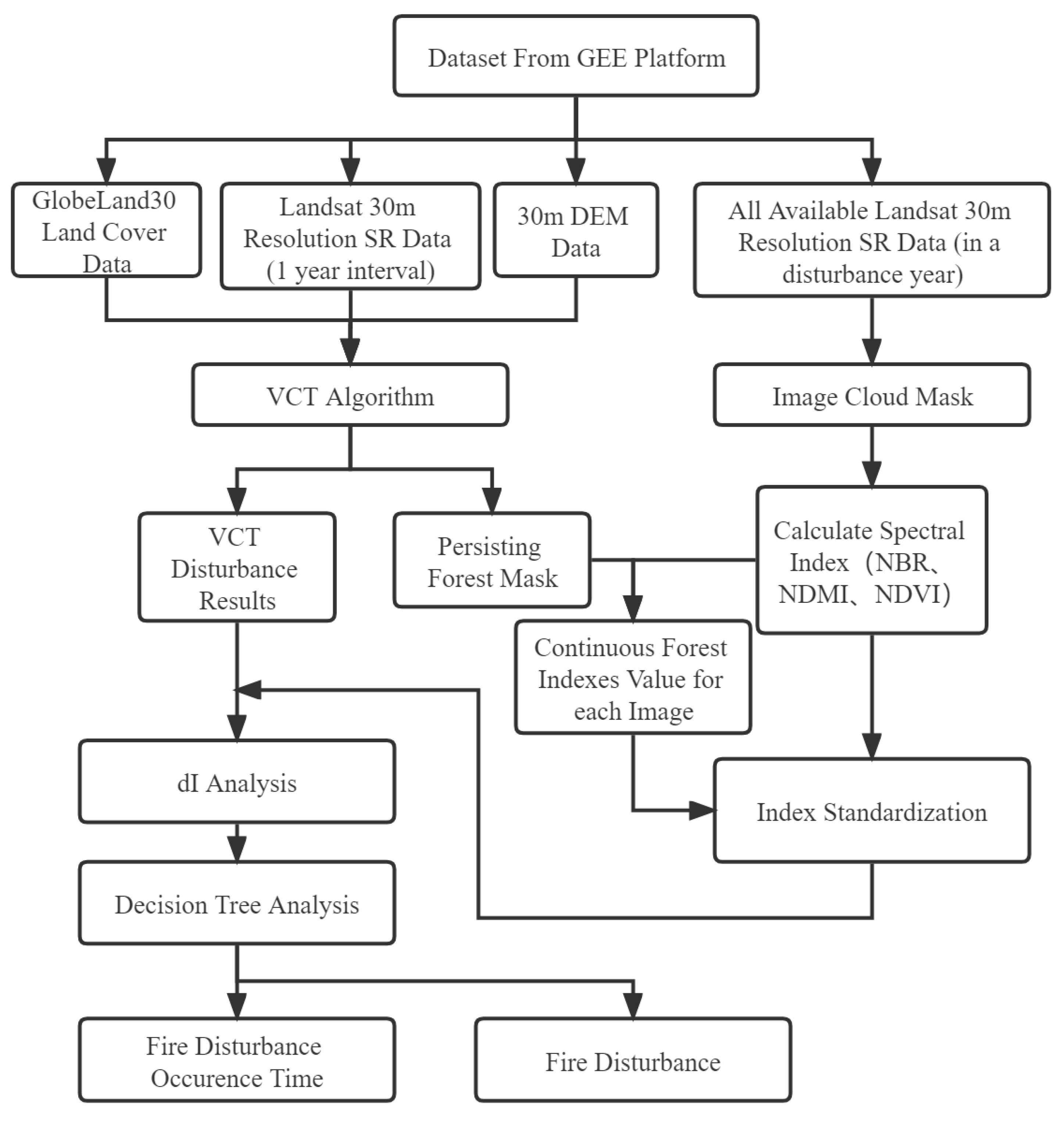
3.5. Flowchart

Figure 2 shows the flowchart of the analysis.

4. Results

4.1. VCT-Mapped Forest Disturbance Events

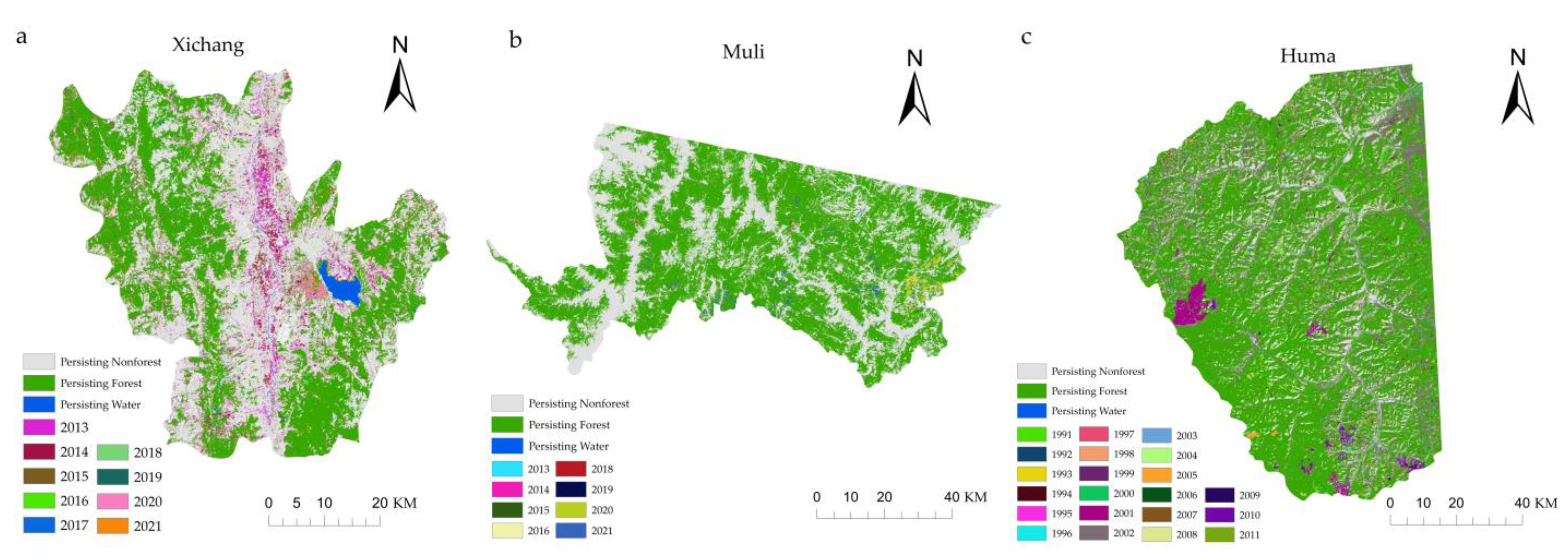
Since the VCT algorithm has been widely used and validated in many regions worldwide [21,42,43,44,45], we used its results in the subsequent analysis without validating them, i.e., we used the persisting forest mask derived from the VCT algorithm in the annual forest disturbance maps. Figure 3 shows the annual disturbance events derived from the VCT in the Xichang, Muli, and Huma regions. The green areas represent persisting forest pixels during the observation period. The gray areas (non-forest) and blue areas (water) were excluded, and the other colors show the forest disturbance events occurring in different years. Due to low image contrast in the first year of the Landsat time-series stacks, none of the disturbance events mapped in the first year (in 2013 in Xichang and Muli and in 1991 in Huma) were included [6].

4.2. Vegetation Index Standardization

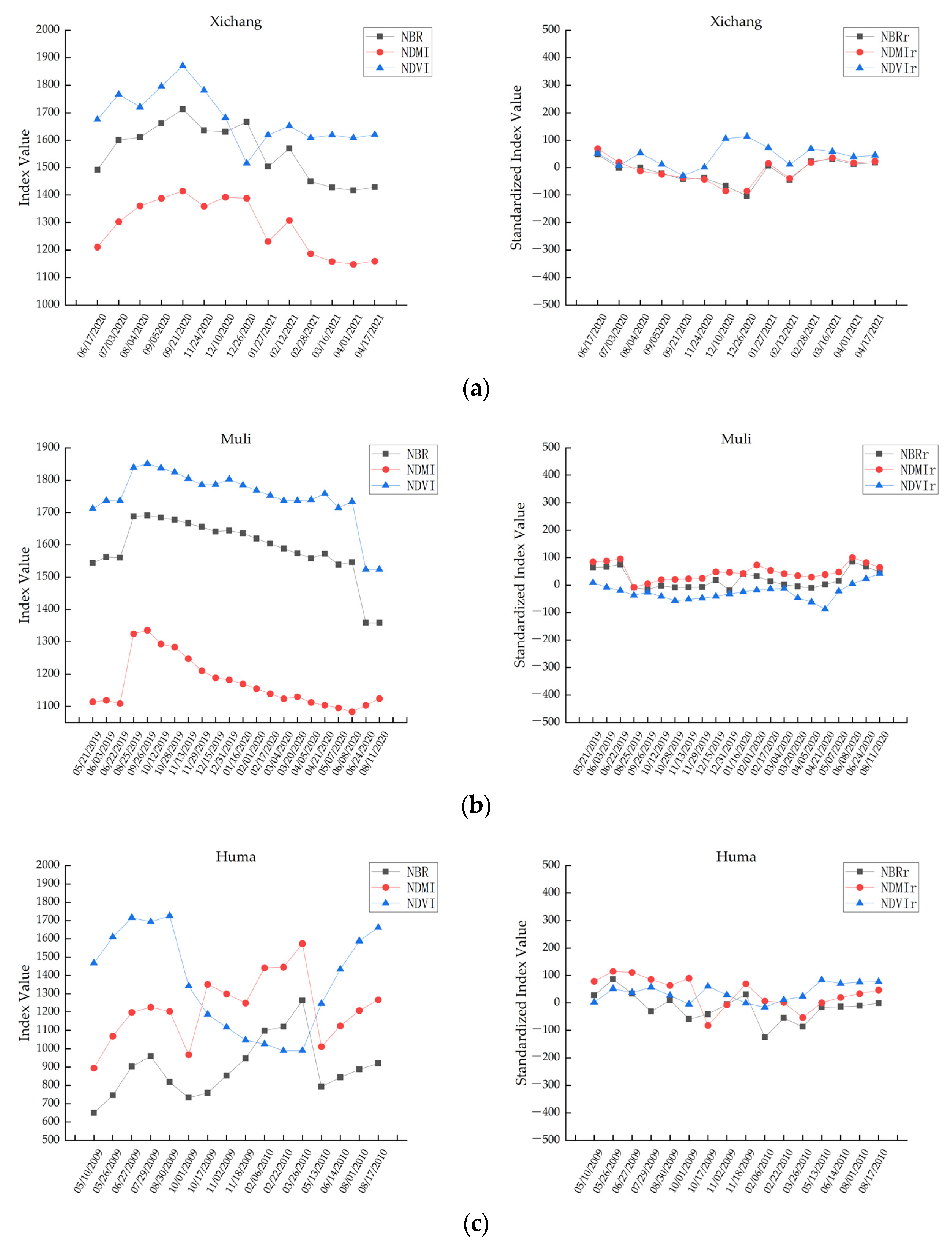
After normalizing the NBR, NDMI, and NDVI values using the persisting forest pixels, the three vegetation indices were less affected by seasonal changes and exhibited higher stability. Figure 4 shows the comparative patterns of the NBR, NDMI, and NDVI for forest pixels in the three regions before and after standardization in a year. The values of the three vegetation indices showed higher variability before normalization but tended to fluctuate from −100 to 100 after normalization, with a mean of about 0.

4.3. Identification of Forest Disturbance Events and Accuracy Assessment

Figure 5 shows that all three indices (dNBRr, dNDMIr, and dNDVIr) remained relatively stable when no forest disturbances occurred, and the values fluctuated around zero with small deviations in Southwestern China. However, the deviations were larger in Northeastern China (Figure 5, Huma), which might be attributed to the presence of snow in the images. When a forest disturbance occurred, the value of the three indices increased abruptly. Thus, it was concluded that the dNBRr, dNDMIr, and dNDVIr could accurately capture forest disturbances (when the value exceeded 190, which was automatically detected by C4.5). The dNBRr showed the highest sensitivity to forest disturbances in Southwestern China because it always had the largest change in the index value when a forest disturbance occurred. In Northeastern China, the dNDMIr exhibited the highest sensitivity to forest disturbances, followed by the dNBRr, and the value of the dNBRr was much larger than the automatically identified threshold of 190. Thus, to maintain the consistency and extensibility of the algorithm, we used the dNBRr threshold of 190 to determine the forest disturbance event to maintain the consistency and extensibility of the algorithm.
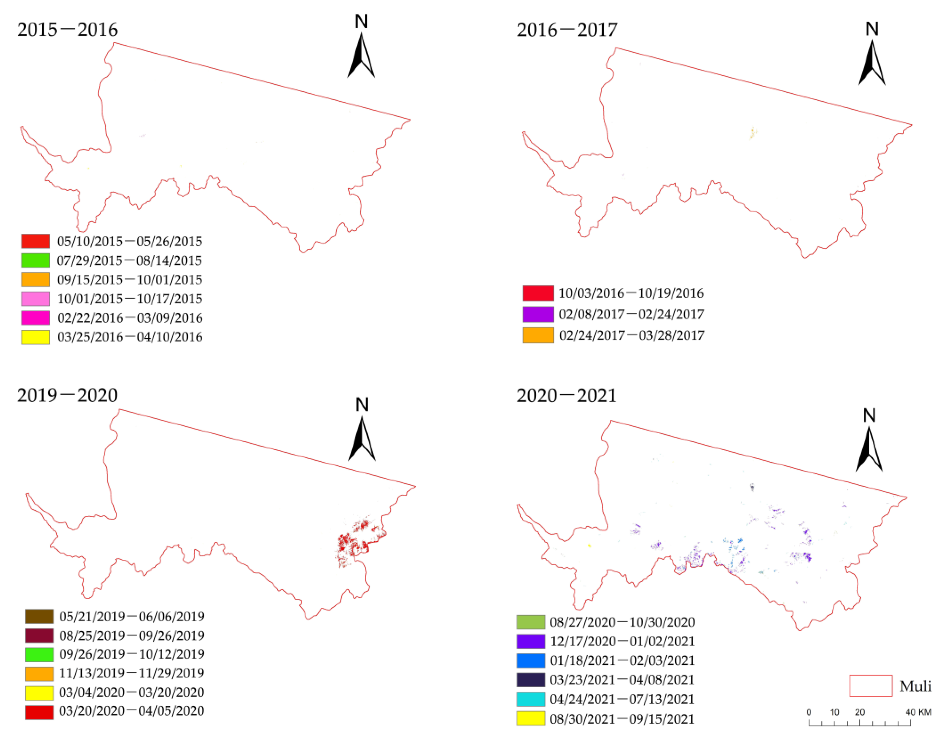
Figure 6, Figure 7 and Figure 8 show the time frames of disturbance events extracted from the dNBRr images using the threshold of 190 for Xichang, Muli, and Huma. Table 5 shows the TA of detecting forest disturbance events in the three study areas. However, due to the limited number of available Landsat images in GEE and cloud contamination, most forest disturbances could not be determined within 16 days, and the period was extended to 2 (32 days) or 3 (48 days) Landsat revisit cycles. The Tas in the Xichang, Muli, and Huma regions were 94.33%, 90.33%, and 89.67%, respectively.

4.4. Fire Disturbance Type Extraction Results and Accuracy Validation

Figure 9 shows the three-dimensional decision boundaries derived from decision tree 2 trained by the Xichang sample data for distinguishing fire disturbance from non-fire disturbance events. Table 6, Table 7 and Table 8 are the confusion matrixes for classifying fire and non-fire disturbance events in Xichang, Muli, and Huma, respectively. Figure 9a shows that three fire pixels are misclassified as non-fire disturbance pixels, and two non-fire disturbance pixels are misclassified as fire disturbance pixels. Overall, the boundaries derived from the decision tree (dNBRr ≥ 580 or dNDMIr ≥ 400 or dNDVIr ≥ 350 for fire disturbance events) performed well in the Xichang region (Figure 9a). Similarly, Figure 9b shows the classification performance for the Muli region. Three fire disturbance pixels are misclassified as non-fire disturbance pixels. Figure 9c shows the classification performance for the Huma region. Only four fire disturbance pixels are misclassified as non-fire disturbance pixels. It was concluded that the automatically derived three-dimensional decision boundaries performed well in distinguishing fire disturbance from non-fire disturbance events in the Xichang, Muli, and Huma regions. The results indicate apparent latitudinal and climatic gradients.
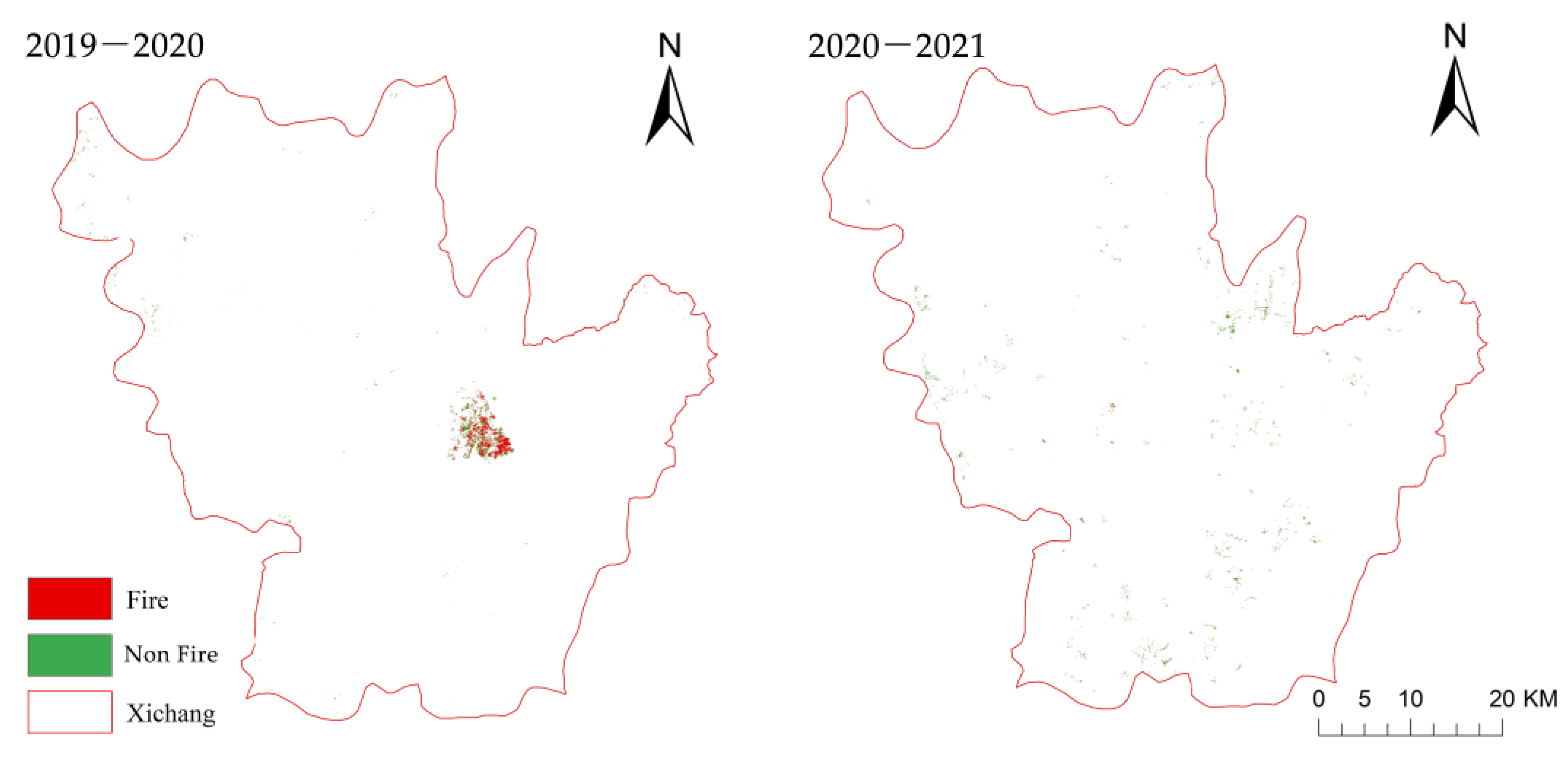
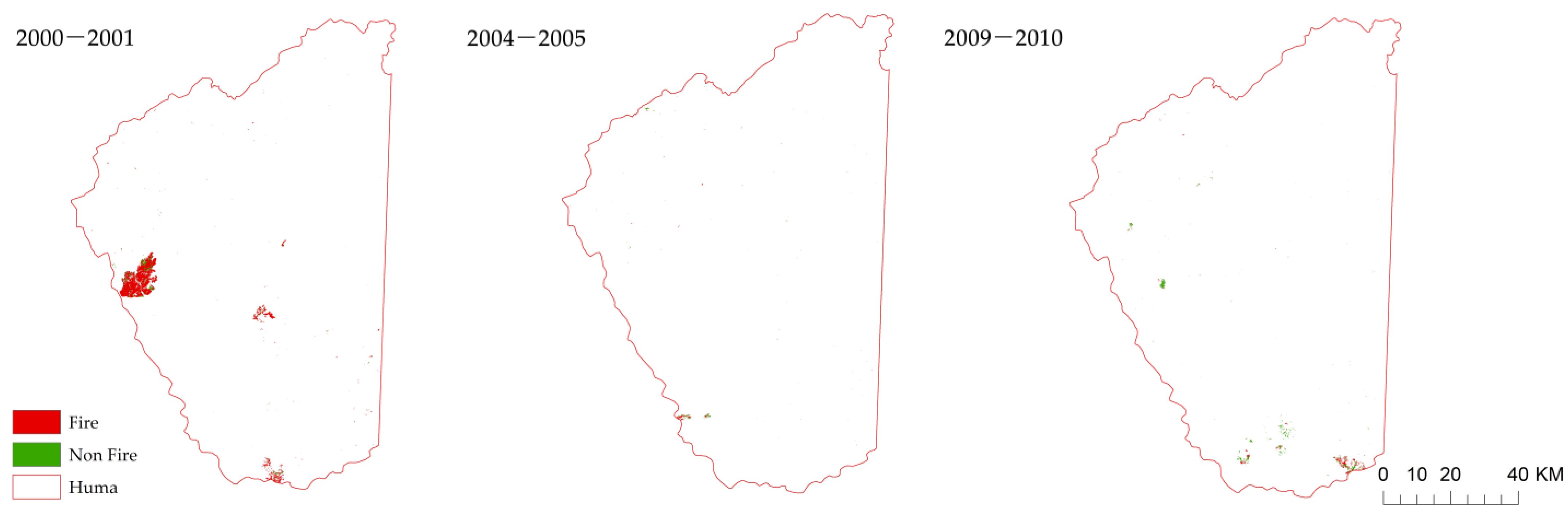
Figure 10, Figure 11 and Figure 12 display the fire disturbance patches and non-fire disturbance patches derived from the three-dimensional decision boundaries of decision tree 2 (dNBRr < 580 or dNDMIr < 400 or dNDVIr < 350 for fire disturbance) in Xichang, Muli, and Huma, respectively. Table 6, Table 7 and Table 8 show that the overall classification accuracy for the three study areas was 85.33%, 89.67%, and 83.67%, and the Kappa coefficients are 0.71, 0.74, and 0.67, respectively.
The fire and non-fire disturbance areas in each year for Xichang, Muli, and Huma are listed in Table 9. Few fire disturbances events occurred from 2020 to 2021 (less than 60 ha), but the area disturbed by fire from 2019 to 2020 was about 630 ha in Xichang. The largest area disturbed by fire in Muli (3820 ha) occurred from 2019 to 2020, followed by 1337 ha from 2020 to 2021. The fire-disturbed areas were small in the other years. Three large fires occurred in Huma from 2000 to 2001, and one occurred between 2009 and 2010, resulting in a relatively large fire-disturbed area in these years.

5. Discussion

5.1. Determining the Occurrence of Disturbances Using All Available Images

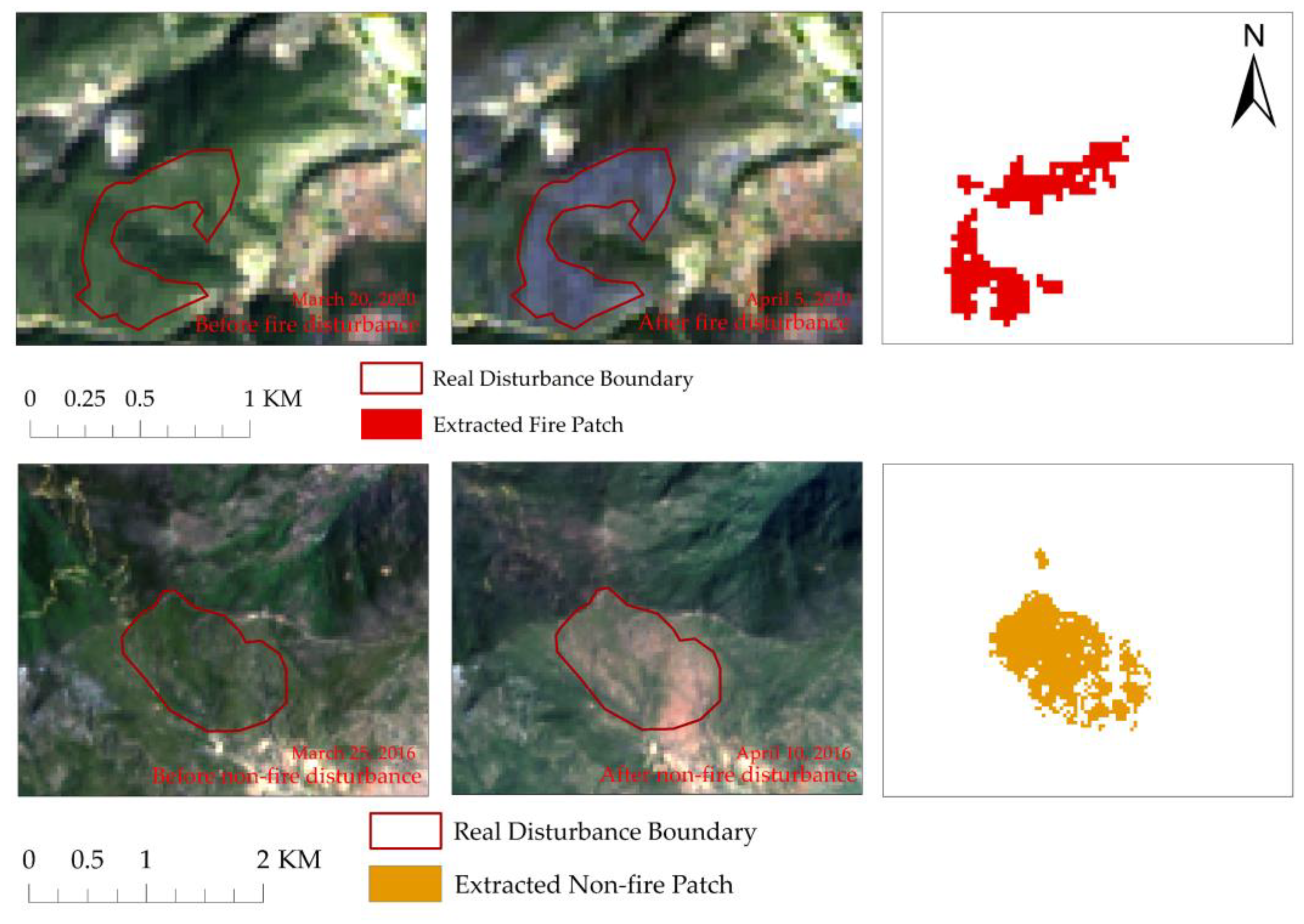
We used the VCT algorithm and all available Landsat time-series images in the GEE platform to determine the occurrence of forest disturbance events between 2 temporally adjacent images (ideally within the 16-day revisit time) (Figure 6, Figure 7 and Figure 8). Some studies extracted forest fire events using VCT and LandTrendr algorithms and Landsat images with 1-year or 2-year intervals [21,55,56,57,58,59]; thus, they could only determine the occurrence of fire disturbances within 1 year. Rose and Nagle used the CCDC method to extract fire events based on all available Landsat image data, but this method requires a large number of disturbance samples [19,60]. Other studies used the BFAST method, which requires 16-day MODIS NDVI time-series data and yields fire disturbance events within a 1-year range [61,62]. In contrast, our proposed framework represents a rapid and convenient approach, which only requires thresholding of normalized vegetation indices for extracting forest fire events using a set of fixed thresholds to narrow the fire occurrence time to a 16-day range under ideal conditions. Figure 13 (the first row) shows the extracted fire patches in the Muli area. The occurrence time of the fire is narrowed down to 16 days (20 March 2020 to 5 April 2020) due to the availability of dense Landsat time-series data in the GEE platform. Data from Landsat 9, which was launched in September 2021, have been available for downloading since February 2022 [63]. Thus, our framework can theoretically narrow down forest disturbances occurring after 30 September 2021 to a period of 8 days if Landsat 8 and Landsat 9 images are used.
Unlike most algorithms based on Landsat time series that can detect forest fire disturbances only within a 1-year period, the proposed framework narrows down this period to 16 or 8 days. This short time window can help reliably extract fire scars and assess post-fire forest loss using remote sensing data. For example, if a forest disturbance occurred within a 16-day or 8-day period, we can compare Landsat-based features, such as NDVI, NDWI, land surface temperature (LST), and NBR before and after the disturbance at the start and end of the time window to determine whether the disturbance is a fire-induced disturbance event or not. The threshold depends largely on the fire severity. If 1-year interval Landsat image pairs are used, the change magnitude of these features is relatively small due to vegetation recovery or changes in precipitation [22,64,65]. Therefore, using a 1-year interval results in low reliability in identifying fire disturbances. In contrast, a short time window enables a more timely assessment of the fire severity change. In addition, information on dominant tree species and tree age in the disturbed areas derived from forest management information systems and species-specific allometric biomass equations can be integrated to obtain an accurate estimate of carbon emissions from fires [66]. However, the vegetation in a disturbance patch can quickly recover during 1 year under favorable temperature and precipitation conditions. For example, João et al. found that different forest types had different recovery speeds. Broadleaf forests and mixed broadleaf-conifer forests required less than 250 days to reach 50% level of pre-fire conditions, while coniferous forests required from 400 to 500 days to reach the same conditions [67]. The proposed method that uses a 16-day or 8-day intervals is more suitable for analyzing the seasonal characteristics of fire occurrences and develop forest fire risk warning and prevention policies and post-fire revegetation measures-based [53,68,69]. For example, if fires frequently occur in a rainy season in an area with flammable tree species, the post-fire revegetation strategy can be adjusted because less moisture is required. Moreover, forest fires are triggered by different factors, such as climate, topography, vegetation type, and economic development status. If the time of the forest fire can be determined more accurately, the relationship between the fire occurrence and these factors can be evaluated to implement fire prevention and suppression measures and post-fire revegetation practices and their assessment [70,71,72,73]. Although MODIS, AVHRR, and FY data have high temporal resolution, their low spatial resolution prevents the detection of small fire events. The fire products also contain mixed pixels, lowering the accuracy of classifying fire patches. Instead, we used Landsat data (30 m spatial resolution) in our study [74,75] because these data are more suitable for extracting burn severity to develop targeted recovery measures [22].

5.2. Extraction of Fire Disturbance Events

We standardized the three vegetation indices using the persisting forest mask extracted from the VCT algorithm and distinguished between fire disturbance and non-fire disturbance events using decision rules and the dI images of the three indices (Figure 10, Figure 11 and Figure 12). Most studies that classified forest disturbance types based on multispectral image data, such as Landsat, distinguished between different forest disturbance types based on a large number of training samples from different images labeled with different forest disturbance types [14,21,25,76,77]. In these studies, it is typically necessary to select training samples from different regions and different dates to reduce the variability between different images. Here, we minimized the differences in the vegetation index values between different images by standardizing the three vegetation indices (Figure 4). This strategy is much less complicated than using a large training sample size. The decision tree rules for extracting forest fire disturbances obtained from the C4.5 data mining tool based on the normalized indices provided high extraction accuracy and were applicable to the three different regions (Xichang and Muli in Southwestern China and Huma in Northeastern China) with apparent latitudinal and climatic gradients (Figure 9 and Figure 13). However, using these decision tree rules to extract fire/non-fire disturbances is dependent on the intensity of the disturbance to some extent. Some low-intensity fire disturbance patches might be misclassified as non-fire disturbances or no disturbances, and some fire events might be missed due to their small size. These conditions may affect the accuracy of the results.
Different forest disturbances require different forest management and restoration measures [25,40,41]. For example, forest fires and deforestation may require reforestation to achieve rapid forest recovery, whereas pests and diseases must be controlled to prevent their spread. The ability to distinguish fire and non-fire disturbance events rapidly and efficiently enables the implementation of targeted preventive and management measures in a timely manner. The three vegetation indices (NBR, NDMI, and NDVI) could distinguish fire from non-fire disturbances. Different non-fire disturbance types, such as clearcuts, pests, and diseases, could be distinguished if spectral features (surface temperature, brightness, and greenness), spatial features (morphological features), and textural features were combined with data from other sources (such as high spatial resolution satellite imagery and LiDAR data) [78,79,80,81]. Additionally, the proposed method depends on the quantity and quality of available Landsat 8 images in GEE for distinguishing fire disturbances and non-fire disturbances.

6. Conclusions

We used the VCT algorithm, Landsat time-series images in the GEE platform, and an efficient and reliable framework for the automatic extraction of forest disturbances. We distinguished between fire disturbances and non-fire disturbances using decision rules obtained from the C4.5 tool. Three vegetation indices were normalized to reduce the variability of the spectral features in different seasons, dates, and regions in a year. Two sets of decision rules were created to determine the occurrence time of disturbance event and separate fire disturbance from non-fire disturbance events. The proposed method narrowed the period for detecting disturbance events down to 16 days or 8 days when Landsat 8 and Landsat 9 images were available. The framework exhibited high accuracy and transferability in the three study areas (Xichang, Muli, and Huma), indicating that the decision trees performed well in different latitudes and climate zones. This study provides a new approach to creating products suitable for implementing targeted forest management policies and measures in different regions.

Author Contributions

Conceptualization, M.L.; methodology, J.Y., N.W., M.S. and M.L.; software, J.Y. and N.D.; validation, J.Y., Q.L. and N.W.; formal analysis, J.Y., M.S. and N.D.; investigation, J.Y., N.W. and Q.L.; resources, J.Y. and N.D.; data curation, J.Y., N.W., M.S. and N.D.; writing—original draft preparation, J.Y. and M.S.; writing—review and editing, J.Y., N.W. and Q.L.; visualization, J.Y., M.S. and Q.L.; supervision, N.W., M.S., Q.L., N.D. and M.L.; project administration, M.L.; funding acquisition, M.L. All authors have read and agreed to the published version of the manuscript.

Funding

This research was jointly funded by the Natural Science Foundation of China, grant number 31971577, and the Priority Academic Program Development of Jiangsu Higher Education Institutions (PAPD).

Institutional Review Board Statement

Not applicable.

Informed Consent Statement

Not applicable.

Data Availability Statement

Not applicable.

Conflicts of Interest

The authors declare no conflict of interest.

References

  1. Liu, N.; Wang, D.; Guo, Q. Exploring the Influence of Large Trees on Temperate Forest Spatial Structure from the Angle of Mingling. For. Ecol. Manag. 2021, 492, 119220. [Google Scholar] [CrossRef]
  2. Nunery, J.S.; Keeton, W.S. Forest Carbon Storage in the Northeastern United States: Net Effects of Harvesting Frequency, Post-Harvest Retention, and Wood Products. For. Ecol. Manag. 2010, 259, 1363–1375. [Google Scholar] [CrossRef]
  3. He, L.; Ivanov, V.Y.; Bohrer, G.; Thomsen, J.E.; Vogel, C.S.; Moghaddam, M. Temporal Dynamics of Soil Moisture in a Northern Temperate Mixed Successional Forest after a Prescribed Intermediate Disturbance. Agric. For. Meteorol. 2013, 180, 22–33. [Google Scholar] [CrossRef]
  4. Eshleman, K.N.; McNeil, B.E.; Townsend, P.A. Validation of a Remote Sensing Based Index of Forest Disturbance Using Streamwater Nitrogen Data. Ecol. Indic. 2009, 9, 476–484. [Google Scholar] [CrossRef]
  5. Elmqvist, T.; Wall, M.; Berggren, A.L.; Blix, L.; Fritioff, Å.; Rinman, U. Tropical Forest Reorganization after Cyclone and Fire Disturbance in Samoa: Remnant Trees as Biological Legacies. Ecol. Soc. 2002, 5, 213–218. [Google Scholar] [CrossRef]
  6. Huang, C.; Goward, S.N.; Masek, J.G.; Thomas, N.; Zhu, Z.; Vogelmann, J.E. An Automated Approach for Reconstructing Recent Forest Disturbance History Using Dense Landsat Time Series Stacks. Remote Sens. Environ. 2010, 114, 183–198. [Google Scholar] [CrossRef]
  7. Heinselman, M.L. Fire in the Virgin Forests of the Boundary Waters Canoe Area, Minnesota. Quat. Res. 1973, 3, 329–382. [Google Scholar] [CrossRef]
  8. Bergeron, Y. The Influence of Island and Mainland Lakeshore Landscapes on Boreal Forest Fire Regimes. Ecology 1991, 72, 1980–1992. [Google Scholar] [CrossRef]
  9. Cao, G. Application of Remote Sensing Technology in Forest Resources Investigation. Remote Sens. 2020, 9, 46. [Google Scholar] [CrossRef]
  10. Herold, M.; Roberts, D.A.; Gardner, M.E.; Dennison, P.E. Spectrometry for Urban Area Remote Sensing–Development and Analysis of a Spectral Library from 350 to 2400 Nm. Remote Sens. Environ. 2004, 91, 304–319. [Google Scholar] [CrossRef]
  11. Martinuzzi, S.; Gould, W.A.; Ramos González, O.M. Land Development, Land Use, and Urban Sprawl in Puerto Rico Integrating Remote Sensing and Population Census Data. Landsc. Urban Plan. 2007, 79, 288–297. [Google Scholar] [CrossRef]
  12. Yang, X.J.; Chang, Z.M.; Zhou, H.; Qu, X.; Li, C.J. Services for Parallel Remote-Sensing Image Processing Based on Computational Grid. Lect. Notes Comput. Sci. 2004, 3252, 689–696. [Google Scholar] [CrossRef]
  13. Mas, J.F. Monitoring Land-Cover Changes: A Comparison of Change Detection Techniques. Int. J. Remote Sens. 1999, 20, 139–152. [Google Scholar] [CrossRef]
  14. Hua, J.; Chen, G.; Yu, L.; Ye, Q.; Jiao, H.; Luo, X. Improved Mapping of Long-Term Forest Disturbance and Recovery Dynamics in the Subtropical China Using All Available Landsat Time-Series Imagery on Google Earth Engine Platform. IEEE J. Sel. Top. Appl. Earth Obs. Remote Sens. 2021, 14, 2754–2768. [Google Scholar] [CrossRef]
  15. Huang, C.; Thomas, N.; Goward, S.N.; Masek, J.G.; Zhu, Z.; Townshend, J.R.G.; Vogelmann, J.E. Automated Masking of Cloud and Cloud Shadow for Forest Change Analysis Using Landsat Images. Int. J. Remote Sens. 2010, 31, 5449–5464. [Google Scholar] [CrossRef]
  16. Gorelick, N.; Hancher, M.; Dixon, M.; Ilyushchenko, S.; Thau, D.; Moore, R. Google Earth Engine: Planetary-Scale Geospatial Analysis for Everyone. Remote Sens. Environ. 2017, 202, 18–27. [Google Scholar] [CrossRef]
  17. Weng, Q.; Fu, P.; Gao, F. Generating Daily Land Surface Temperature at Landsat Resolution by Fusing Landsat and MODIS Data. Remote Sens. Environ. 2014, 145, 55–67. [Google Scholar] [CrossRef]
  18. Kennedy, R.E.; Yang, Z.; Cohen, W.B. Detecting Trends in Forest Disturbance and Recovery Using Yearly Landsat Time Series: 1. LandTrendr-Temporal Segmentation Algorithms. Remote Sens. Environ. 2010, 114, 2897–2910. [Google Scholar] [CrossRef]
  19. Zhu, Z.; Woodcock, C.E. Continuous Change Detection and Classification of Land Cover Using All Available Landsat Data. Remote Sens. Environ. 2014, 144, 152–171. [Google Scholar] [CrossRef] [Green Version]
  20. DeVries, B.; Verbesselt, J.; Kooistra, L.; Herold, M. Robust Monitoring of Small-Scale Forest Disturbances in a Tropical Montane Forest Using Landsat Time Series. Remote Sens. Environ. 2015, 161, 107–121. [Google Scholar] [CrossRef]
  21. Zhao, F.; Huang, C.; Zhu, Z. Use of Vegetation Change Tracker and Support Vector Machine to Map Disturbance Types in Greater Yellowstone Ecosystems in a 1984-2010 Landsat Time Series. IEEE Geosci. Remote Sens. Lett. 2015, 12, 1650–1654. [Google Scholar] [CrossRef]
  22. Miller, J.D.; Thode, A.E. Quantifying Burn Severity in a Heterogeneous Landscape with a Relative Version of the Delta Normalized Burn Ratio (DNBR). Remote Sens. Environ. 2007, 109, 66–80. [Google Scholar] [CrossRef]
  23. Qarallah, B.; Al-Ajlouni, M.; Al-Awasi, A.; Alkarmy, M.; Al-Qudah, E.; Naser, A.B.; Al-Assaf, A.; Gevaert, C.M.; Al Asmar, Y.; Belgiu, M.; et al. Evaluating Post-Fire Recovery of Latroon Dry Forest Using Landsat ETM+, Unmanned Aerial Vehicle and Field Survey Data. J. Arid Environ. 2021, 193, 104587. [Google Scholar] [CrossRef]
  24. Bar, S.; Parida, B.R.; Pandey, A.C. Landsat-8 and Sentinel-2 Based Forest Fire Burn Area Mapping Using Machine Learning Algorithms on GEE Cloud Platform over Uttarakhand, Western Himalaya. Remote Sens. Appl. Soc. Environ. 2020, 18, 100324. [Google Scholar] [CrossRef]
  25. Li, Y.; Wu, Z.; Xu, X.; Fan, H.; Tong, X.; Liu, J. Forest Disturbances and the Attribution Derived from Yearly Landsat Time Series over 1990–2020 in the Hengduan Mountains Region of Southwest China. For. Ecosyst. 2021, 8, 73. [Google Scholar] [CrossRef]
  26. Lu, D.; Mausel, P.; Brondízio, E.; Moran, E. Change Detection Techniques. Int. J. Remote Sens. 2004, 25, 2365–2401. [Google Scholar] [CrossRef]
  27. Szajewska, A. Classification of a Burnt Area Based on Spectral Images. MATEC Web Conf. 2018, 247, 00017. [Google Scholar] [CrossRef] [Green Version]
  28. Soverel, N.O.; Perrakis, D.D.B.; Coops, N.C. Estimating Burn Severity from Landsat DNBR and RdNBR Indices across Western Canada. Remote Sens. Environ. 2010, 114, 1896–1909. [Google Scholar] [CrossRef]
  29. Hais, M.; Jonášová, M.; Langhammer, J.; Kučera, T. Comparison of Two Types of Forest Disturbance Using Multitemporal Landsat TM/ETM+ Imagery and Field Vegetation Data. Remote Sens. Environ. 2009, 113, 835–845. [Google Scholar] [CrossRef]
  30. Cohen, W.B.; Yang, Z.; Kennedy, R. Detecting Trends in Forest Disturbance and Recovery Using Yearly Landsat Time Series: 2. TimeSync–Tools for Calibration and Validation. Remote Sens. Environ. 2010, 114, 2911–2924. [Google Scholar] [CrossRef]
  31. Chu, T.; Guo, X. Remote Sensing Techniques in Monitoring Post-Fire Effects and Patterns of Forest Recovery in Boreal Forest Regions: A Review. Remote Sens. 2013, 6, 470–520. [Google Scholar] [CrossRef] [Green Version]
  32. Key, C.H.; Benson, N.C. Landscape Assessment (LA) Sampling and Analysis Methods. USDA For. Serv.-Gen. Tech. Rep. RMRS-GTR 2006, 1, 11–12. [Google Scholar]
  33. Lentile, L.B.; Holden, Z.A.; Smith, A.M.S.; Falkowski, M.J.; Hudak, A.T.; Morgan, P.; Lewis, S.A.; Gessler, P.E.; Benson, N.C. Remote Sensing Techniques to Assess Active Fire Characteristics and Post-Fire Effects. Int. J. Wildland Fire 2006, 15, 319–345. [Google Scholar] [CrossRef]
  34. Jin, S.; Sader, S.A. Comparison of Time Series Tasseled Cap Wetness and the Normalized Difference Moisture Index in Detecting Forest Disturbances. Remote Sens. Environ. 2005, 94, 364–372. [Google Scholar] [CrossRef]
  35. Gao, Y.; Quevedo, A.; Szantoi, Z.; Skutsch, M. Monitoring Forest Disturbance Using Time-Series MODIS NDVI in Michoacán, Mexico. Geocarto Int. 2021, 36, 1768–1784. [Google Scholar] [CrossRef]
  36. Doi, R. Simple Luminosity Normalization of Greenness, Yellowness and Redness/Greenness for Comparison of Leaf Spectral Profiles in Multi-Temporally Acquired Remote Sensing Images. J. Biosci. 2012, 37, 723–730. [Google Scholar] [CrossRef]
  37. Healey, J.S.; Baranchuk, A.; Crystal, E.; Morillo, C.A.; Garfinkle, M.; Yusuf, S.; Connolly, S.J. Prevention of Atrial Fibrillation with Angiotensin-Converting Enzyme Inhibitors and Angiotensin Receptor Blockers: A Meta-Analysis. J. Am. Coll. Cardiol. 2005, 45, 1832–1839. [Google Scholar] [CrossRef] [Green Version]
  38. Huang, C.; Goward, S.N.; Schleeweis, K.; Thomas, N.; Masek, J.G.; Zhu, Z. Dynamics of National Forests Assessed Using the Landsat Record: Case Studies in Eastern United States. Remote Sens. Environ. 2009, 113, 1430–1442. [Google Scholar] [CrossRef]
  39. Ferreira, L.G.; Yoshioka, H.; Huete, A.; Sano, E.E. Seasonal Landscape and Spectral Vegetation Index Dynamics in the Brazilian Cerrado: An Analysis within the Large-Scale Biosphere-Atmosphere Experiment in Amazônia (LBA). Remote Sens. Environ. 2003, 87, 534–550. [Google Scholar] [CrossRef]
  40. Du, J.; Wang, K.; Cui, B. Attribution of the Extreme Drought-Related Risk of Wildfires in Spring 2019 over Southwest China. Bull. Am. Meteorol. Soc. 2021, 102, S83–S90. [Google Scholar] [CrossRef]
  41. Wu, L.; Li, Z.; Liu, X.; Zhu, L.; Tang, Y.; Zhang, B.; Xu, B.; Liu, M.; Meng, Y.; Liu, B. Multi-Type Forest Change Detection Using BFAST and Monthly Landsat Time Series for Monitoring Spatiotemporal Dynamics of Forests in Subtropical Wetland. Remote Sens. 2020, 12, 341. [Google Scholar] [CrossRef]
  42. Vermote, E.; Justice, C.; Claverie, M.; Franch, B. Preliminary Analysis of the Performance of the Landsat 8/OLI Land Surface Reflectance Product. Remote Sens. Environ. 2016, 185, 46–56. [Google Scholar] [CrossRef]
  43. Masek, J.G.; Vermote, E.F.; Saleous, N.E.; Wolfe, R.; Hall, F.G.; Huemmrich, K.F.; Gao, F.; Kutler, J.; Lim, T.K. A Landsat Surface Reflectance Dataset for North America, 1990-2000. IEEE Geosci. Remote Sens. Lett. 2006, 3, 68–72. [Google Scholar] [CrossRef]
  44. Masek, J. Automated Registration and Orthorectification Package for Landsat and Landsat-like Data Processing. J. Appl. Remote Sens. 2009, 3, 033515. [Google Scholar] [CrossRef]
  45. Tan, B.; Wolfe, R.; Masek, J.; Gao, F.; Vermote, E.F. An Illumination Correction Algorithm on Landsat-TM Data. Int. Geosci. Remote Sens. Symp. (IGARSS) 2010, 1964–1967. [Google Scholar] [CrossRef]
  46. Shen, W.; Li, M.; Wei, A. Spatio-Temporal Variations in Plantation Forests’ Disturbance and Recovery of Northern Guangdong Province Using Yearly Landsat Time Series Observations (1986–2015). Chin. Geogr. Sci. 2017, 27, 600–613. [Google Scholar] [CrossRef]
  47. Kauffman, J.S.; Prisley, S.P. Automated Estimation of Forest Stand Age Using Vegetation Change Tracker and Machine Learning. Math. Comput. For. Nat.-Resour. Sci. 2016, 8, 4–13. [Google Scholar]
  48. Meng, R.; Dennison, P.E.; Huang, C.; Moritz, M.A.; D’Antonio, C. Effects of Fire Severity and Post-Fire Climate on Short-Term Vegetation Recovery of Mixed-Conifer and Red Fir Forests in the Sierra Nevada Mountains of California. Remote Sens. Environ. 2015, 171, 311–325. [Google Scholar] [CrossRef]
  49. Qiu, J.; Wang, H.; Shen, W.; Zhang, Y.; Su, H.; Li, M. Quantifying Forest Fire and Post-Fire Vegetation Recovery in the Daxing’anling Area of Northeastern China Using Landsat Time-Series Data and Machine Learning. Remote Sens. 2021, 13, 792. [Google Scholar] [CrossRef]
  50. García, M.J.L.; Caselles, V. Mapping Burns and Natural Reforestation Using Thematic Mapper Data. Geocarto Int. 1991, 6, 31–37. [Google Scholar] [CrossRef]
  51. Gao, B.C. NDWI—A Normalized Difference Water Index for Remote Sensing of Vegetation Liquid Water from Space. Remote Sens. Environ. 1996, 58, 257–266. [Google Scholar] [CrossRef]
  52. Carlson, T.N.; Ripley, D.A. On the Relation between NDVI, Fractional Vegetation Cover, and Leaf Area Index. Remote Sens. Environ. 1997, 62, 241–252. [Google Scholar] [CrossRef]
  53. Gao, C.; An, R.; Wang, W.; Shi, C.; Wang, M.; Liu, K.; Wu, X.; Wu, G.; Shu, L. Asymmetrical Lightning Fire Season Expansion in the Boreal Forest of Northeast China. Forests 2021, 12, 1023. [Google Scholar] [CrossRef]
  54. Quinlan, J.R. C4.5: Programs for Machine Learning (Morgan Kaufmann Series in Machine Learning). Morgan Kaufmann San Mateo Calif. 1992, 302, 235–240. [Google Scholar]
  55. Huang, C.; Goward, S.N.; Masek, J.G.; Gao, F.; Vermote, E.F.; Thomas, N.; Schleeweis, K.; Kennedy, R.E.; Zhu, Z.; Eidenshink, J.C.; et al. Development of Time Series Stacks of Landsat Images for Reconstructing Forest Disturbance History. Int. J. Digit. Earth 2009, 2, 195–218. [Google Scholar] [CrossRef]
  56. Pflugmacher, D.; Cohen, W.B.; Kennedy, R.E.; Yang, Z. Using Landsat-Derived Disturbance and Recovery History and Lidar to Map Forest Biomass Dynamics. Remote Sens. Environ. 2014, 151, 124–137. [Google Scholar] [CrossRef]
  57. Chen, S.; Woodcock, C.E.; Bullock, E.L.; Arévalo, P.; Torchinava, P.; Peng, S.; Olofsson, P. Monitoring Temperate Forest Degradation on Google Earth Engine Using Landsat Time Series Analysis. Remote Sens. Environ. 2021, 265, 112648. [Google Scholar] [CrossRef]
  58. Chen, N.; Tsendbazar, N.E.; Hamunyela, E.; Verbesselt, J.; Herold, M. Sub-Annual Tropical Forest Disturbance Monitoring Using Harmonized Landsat and Sentinel-2 Data. Int. J. Appl. Earth Obs. Geoinf. 2021, 102, 102386. [Google Scholar] [CrossRef]
  59. Quintero, N.; Viedma, O.; Urbieta, I.R.; Moreno, J.M. Assessing Landscape Fire Hazard by Multitemporal Automatic Classification of Landsat Time Series Using the Google Earth Engine in West-Central Spain. Forests 2019, 10, 518. [Google Scholar] [CrossRef] [Green Version]
  60. Rose, M.B.; Nagle, N.N. Characterizing Forest Dynamics with Landsat-Derived Phenology Curves. Remote Sens. 2021, 13, 267. [Google Scholar] [CrossRef]
  61. Verbesselt, J.; Hyndman, R.; Newnham, G.; Culvenor, D. Detecting Trend and Seasonal Changes in Satellite Image Time Series. Remote Sens. Environ. 2010, 114, 106–115. [Google Scholar] [CrossRef]
  62. Katagis, T.; Gitas, I.Z.; Toukiloglou, P.; Veraverbeke, S.; Goossens, R. Trend Analysis of Medium- and Coarse-Resolution Time Series Image Data for Burned Area Mapping in a Mediterranean Ecosystem. Int. J. Wildland Fire 2014, 23, 668–677. [Google Scholar] [CrossRef] [Green Version]
  63. Masek, J.G.; Wulder, M.A.; Markham, B.; McCorkel, J.; Crawford, C.J.; Storey, J.; Jenstrom, D.T. Landsat 9: Empowering Open Science and Applications through Continuity. Remote Sens. Environ. 2020, 248, 111968. [Google Scholar] [CrossRef]
  64. Caccamo, G.; Bradstock, R.; Collins, L.; Penman, T.; Watson, P. Using MODIS Data to Analyse Post-Fire Vegetation Recovery in Australian Eucalypt Forests. J. Spat. Sci. 2015, 60, 341–352. [Google Scholar] [CrossRef]
  65. Bright, B.C.; Hudak, A.T.; Kennedy, R.E.; Braaten, J.D.; Henareh Khalyani, A. Examining Post-Fire Vegetation Recovery with Landsat Time Series Analysis in Three Western North American Forest Types. Fire Ecol. 2019, 15, 8. [Google Scholar] [CrossRef] [Green Version]
  66. Tepley, A.J.; Thomann, E.; Veblen, T.T.; Perry, G.L.W.; Holz, A.; Paritsis, J.; Kitzberger, T.; Anderson-Teixeira, K.J. Influences of Fire–Vegetation Feedbacks and Post-Fire Recovery Rates on Forest Landscape Vulnerability to Altered Fire Regimes. J. Ecol. 2018, 106, 1925–1940. [Google Scholar] [CrossRef] [Green Version]
  67. João, T.; João, G.; Bruno, M.; João, H. Indicator-Based Assessment of Post-Fire Recovery Dynamics Using Satellite NDVI Time-Series. Ecol. Indic. 2018, 89, 199–212. [Google Scholar] [CrossRef]
  68. Veraverbeke, S.; Rogers, B.M.; Goulden, M.L.; Jandt, R.R.; Miller, C.E.; Wiggins, E.B.; Randerson, J.T. Lightning as a Major Driver of Recent Large Fire Years in North American Boreal Forests. Nat. Clim. Chang. 2017, 7, 529–534. [Google Scholar] [CrossRef]
  69. Sparks, J.C.; Masters, R.E.; Engle, D.M.; Bukenhofer, G.A. Season of Burn Influences Fire Behavior and Fuel Consumption in Restored Shortleaf Pine–Grassland Communities. Restor. Ecol. 2002, 10, 714–722. [Google Scholar] [CrossRef]
  70. Kirchmeier-Young, M.C.; Zwiers, F.W.; Gillett, N.P.; Cannon, A.J. Attributing Extreme Fire Risk in Western Canada to Human Emissions. Clim. Change 2017, 144, 365–379. [Google Scholar] [CrossRef] [Green Version]
  71. Kupriyanov, D.A.; Novenko, E.Y. Reconstruction of the Holocene Dynamics of Forest Fires in the Central Part of Meshcherskaya Lowlands According to Antracological Analysis. Contemp. Probl. Ecol. 2019, 12, 204–212. [Google Scholar] [CrossRef]
  72. Daşdemir, İ.; Aydın, F.; Ertuğrul, M. Factors Affecting the Behavior of Large Forest Fires in Turkey. Environ. Manag. 2021, 67, 162–175. [Google Scholar] [CrossRef] [PubMed]
  73. Kutiel, H. Weather Conditions and Forest Fire Propagation-the Case of the Carmel Fire, December 2010. Isr. J. Ecol. Evol. 2012, 58, 113–122. [Google Scholar] [CrossRef]
  74. Hua, L.; Shao, G. The Progress of Operational Forest Fire Monitoring with Infrared Remote Sensing. J. For. Res. 2017, 28, 215–229. [Google Scholar] [CrossRef]
  75. Krylov, A.; McCarty, J.L.; Potapov, P.; Loboda, T.; Tyukavina, A.; Turubanova, S.; Hansen, M.C. Remote Sensing Estimates of Stand-Replacement Fires in Russia, 2002-2011. Environ. Res. Lett. 2014, 9, 105007. [Google Scholar] [CrossRef]
  76. Chen, X.; Zhao, W.; Chen, J.; Qu, Y.; Wu, D.; Chen, X. Mapping Large-Scale Forest Disturbance Types with Multi-Temporal Cnn Framework. Remote Sens. 2021, 13, 5177. [Google Scholar] [CrossRef]
  77. Pouliot, D.; Latifovic, R.; Fernandes, R.; Olthof, I. Evaluation of Annual Forest Disturbance Monitoring Using a Static Decision Tree Approach and 250 m MODIS Data. Remote Sens. Environ. 2009, 113, 1749–1759. [Google Scholar] [CrossRef]
  78. Shimizu, K.; Ahmed, O.S.; Ponce-Hernandez, R.; Ota, T.; Win, Z.C.; Mizoue, N.; Yoshida, S. Attribution of Disturbance Agents to Forest Change Using a Landsat Time Series in Tropical Seasonal Forests in the Bago Mountains, Myanmar. Forests 2017, 8, 218. [Google Scholar] [CrossRef]
  79. Zald, H.S.J.; Ohmann, J.L.; Roberts, H.M.; Gregory, M.J.; Henderson, E.B.; McGaughey, R.J.; Braaten, J. Influence of Lidar, Landsat Imagery, Disturbance History, Plot Location Accuracy, and Plot Size on Accuracy of Imputation Maps of Forest Composition and Structure. Remote Sens. Environ. 2014, 143, 26–38. [Google Scholar] [CrossRef]
  80. Stewart, B.P.; Wulder, M.A.; McDermid, G.J.; Nelson, T. Disturbance Capture and Attribution through the Integration of Landsat and IRS-1C Imagery. Can. J. Remote Sens. 2009, 35, 523–533. [Google Scholar] [CrossRef]
  81. Ahmed, O.S.; Franklin, S.E.; Wulder, M.A. Interpretation of Forest Disturbance Using a Time Series of Landsat Imagery and Canopy Structure from Airborne Lidar. Can. J. Remote Sens. 2014, 39, 521–542. [Google Scholar] [CrossRef]
Figure 1. Map of the study areas and the historical forest disturbance events.
Remotesensing 15 00413 g001
Figure 2. Workflow of the analysis.
Remotesensing 15 00413 g002
Figure 3. Forest change analysis results derived from VCT algorithm. (a) Xichang; (b) Muli; (c) Huma.
Remotesensing 15 00413 g003
Figure 4. Effects of normalizing the vegetation indices in (a) Xichang, (b) Muli and (c) Huma.
Remotesensing 15 00413 g004
Figure 5. Identification of forest disturbance events based on the dI values of disturbed/non-disturbed forest pixels in (a) Xichang, (b) Muli and (c) Huma. The value of 190 is the dNBRr threshold identified by decision tree 1 and used to determine forest disturbances. If the dNBRr value exceeds 190, the forest disturbance occurred between this date and the next Landsat acquisition time.
Remotesensing 15 00413 g005
Figure 6. The disturbance events in different years in Xichang using the dNBRr threshold of 190.
Remotesensing 15 00413 g006
Figure 7. The disturbance events in different years in Muli using the dNBRr threshold of 190.
Remotesensing 15 00413 g007
Figure 8. The disturbance events in different years in Huma using the dNBRr threshold of 190.
Remotesensing 15 00413 g008
Figure 9. The three-dimensional decision boundaries for distinguishing fire disturbance events from non-fire disturbance events using the training data from Xichang and validated by independent data from (a) Xichang, (b) Muli and (c) Huma. Note: 580, 400, and 350 are the decision tree thresholds obtained from the Xichang sample pixels. Disturbed pixels with dNBRr < 580 or dNDMIr < 400 or dNDVIr < 350 are fire disturbance pixels, and the other pixels are non-fire disturbance pixels.
Remotesensing 15 00413 g009
Figure 10. The extracted fire/non-fire disturbance events in Xichang derived from the three-dimensional decision boundaries.
Remotesensing 15 00413 g010
Figure 11. The extracted fire/non-fire disturbance events in Muli derived from the three-dimensional decision boundaries.
Remotesensing 15 00413 g011
Figure 12. The extracted fire/non-fire disturbance events in Huma derived from the three-dimensional decision boundaries.
Remotesensing 15 00413 g012
Figure 13. Effectiveness of extracting different forest disturbance types using the three-dimensional decision boundaries.
Remotesensing 15 00413 g013
Table 1. Landsat images used to extract masks of persisting forest areas using the VCT algorithm.
AreaPath/RowSensorAcquisition DateCloud %
Xichang130/041OLI14 June 20130.41%
130/041OLI10 June 20143.50%
130/041OLI26 October 20155.35%
130/041OLI5 May 201610.75%
130/041OLI9 June 201721.07%
130/041OLI11 May 201818.36%
130/041OLI18 August 201923.64%
130/041OLI1 June 202047.87%
130/041OLI3 May 202124.38%
Muli131/041OLI11 October 20130.69%
131/041OLI28 September 20147.47%
131/041OLI10 May 20151.27%
131/041OLI3 October 20166.59%
131/041OLI25 October 20180.17%
131/041OLI21 May 20193.60%
131/041OLI27 August 20201.24%
131/041OLI2 November 20212.51%
Huma122/024TM29 August 199112.00%
122/024TM15 August 199216.00%
122/024TM18 August 19938.00%
122/024TM4 July 19942.00%
122/024TM11 October 19950.00%
122/024TM10 August 19960.00%
122/024TM29 August 19970.00%
122/024TM16 August 19981.00%
122/024TM2 July 19990.00%
122/024TM20 June 20000.00%
122/024TM24 August 20010.00%
122/024TM28 September 20023.00%
122/024TM11 June 20034.00%
122/024TM13 June 20041.00%
122/024TM2 July 20056.00%
122/024TM5 July 20060.00%
122/024TM24 July 200722.00%
122/024TM28 September 20081.00%
122/024TM1 February 20091.00%
122/024TM2 September 20103.00%
122/024TM3 July 20111.00%
Table 2. Amount of available Landsat images in each disturbance year for extracting forest fire events at the three sites using GEE.
AreaPath/RowDisturbance YearNumber of Images
Xichang130/0412019–202016
2020–202114
Muli131/0412015–201620
2016–201835
2019–202021
2020–202122
Huma122/0242000–200117
2004–200515
2009–201016
Table 3. Historical forest disturbance data in the three study areas to develop and validate the fire identification model.
Path/RowDisturbance YearNumber of Fire PatchesNumber of Non-Fire Patches
130/0412019–202011
2020–202101
131/0412015–201611
2016–201821
2019–202030
2020–202122
122/0242000–200130
2004–200511
2009–201014
Table 4. Training samples from the Xichang region for creating the decision trees.
AreaDisturbance TypeNumber of Sample Pixels
XichangDisturbedFire50100
Non-fire50
Not disturbed 100
Table 5. Temporal accuracy of forest disturbance events in Xichang, Muli, and Huma.
AreaNumber of Temporally Matched PixelsNumber of Temporally Mismatched Pixels Temporal Accuracy
Xichang2831794.33%
Muli2712990.33%
Huma2693189.67%
Table 6. Confusion matrix for fire/non-fire disturbance classification in Xichang.
Reference Data
Disturbance TypeFireNon-Fire User’s Accuracy
Fire13716 89.54%
Non-fire28119 80.95%
Producer’s Accuracy83.03%88.15%Overall85.33%
Kappa0.71
Table 7. Confusion matrix for fire/non-fire disturbance classification in Muli.
Reference Data
Disturbance TypeFireNon-Fire User’s Accuracy
Fire20415 93.15%
Non-fire1665 80.25%
Producer’s Accuracy92.73%81.25%Overall89.67%
Kappa0.74
Table 8. Confusion matrix for fire/non-fire disturbance classification in Huma.
Reference Data
Disturbance TypeFireNon-Fire User’s Accuracy
Fire15324 87.01%
Non-fire2796 78.89%
Producer’s Accuracy85.56%80.83%Overall83.67%
Kappa0.67
Table 9. Fire-/Non-fire-disturbed areas in different years in Xichang, Muli, and Huma.
AreaYearFire-Disturbed Area (ha)Non-Fire-Disturbed Area (ha)Total Disturbed Area (ha)
Xichang2019–2020629.64517.231146.87
2020–202156.16274.32330.48
Muli2015–201619.6252.9272.54
2016–201760.7563.99124.74
2019–20203822.75292.864115.61
2020–202113372497.413874.41
Huma2000–20016866.46522.817389.27
2004–2005291.51169.38460.89
2009–20101266.21984.602250.81
Disclaimer/Publisher’s Note: The statements, opinions and data contained in all publications are solely those of the individual author(s) and contributor(s) and not of MDPI and/or the editor(s). MDPI and/or the editor(s) disclaim responsibility for any injury to people or property resulting from any ideas, methods, instructions or products referred to in the content.