Reconstruction of LoD-2 Building Models Guided by Façade Structures from Oblique Photogrammetric Point Cloud

Abstract

Due to the façade visibility, intuitive expression, and multi-view redundancy, oblique photogrammetry can provide optional data for large-scale urban LoD-2 reconstruction. However, the inherent noise in oblique photogrammetric point cloud resulting from the image-dense matching limits further model reconstruction applications. Thus, this paper proposes a novel method for the efficient reconstruction of LoD-2 building models guided by façade structures from an oblique photogrammetric point cloud. First, a building planar layout is constructed combined with footprint data and the vertical planes of the building based on spatial consistency constraints. The cells in the planar layout represent roof structures with a distinct altitude difference. Then, we introduce regularity constraints and a binary integer programming model to abstract the façade with the best-fitting monotonic regularized profiles. Combined with the planar layout and regularized profiles, a 2D building topology is constructed. Finally, the vertices of building roof facets can be derived from the 2D building topology, thus generating a LoD-2 building model. Experimental results using real datasets indicate that the proposed method can generate reliable reconstruction results compared with two state-of-the-art methods.

1. Introduction

According to the OGC (the Open Geospatial Consortium) standard CityGML (City Geography Markup Language) [1], 3D models of buildings can be divided into multiple levels of details (LoDs), with different geometric and semantic information for varying levels of application [2]. The LoD-2 models, which distinguish between the roof and façade of buildings, form the skeleton structure of a smart city and are most widely used in urban construction and management [3]. With the rapid development of aerial vehicles and sensors, point clouds have become the primary data for three-dimensional (3D) urban reconstruction [4,5,6] while enabling automated 3D urban reconstruction. Light detection and ranging (LiDAR) [7,8], as an important means of 3D point cloud data acquisition, can directly obtain the position of the target, obviating the complex procedure of solving the image correspondence. Airborne laser scanning (ALS) point clouds have been widely used for 3D building reconstruction in urban areas [9] because of their short acquisition period and high accuracy. However, building façades are often missing from ALS data, especially for tall buildings [10]. In contrast, the popular oblique photogrammetry system usually carries multiple sensors with different perspectives on the airborne oblique system to collect images simultaneously [11]. Due to oblique images’ perception for complex scenes in a wide range with high accuracy, the dense matching point clouds [12] can represent continuous surfaces containing roofs and façades. Oblique photogrammetry has emerged as a promising technology for detailed 3D urban modeling [13].

A great amount of research has been carried out on the reconstruction of 3D buildings, and significant progress has been made in LoDs [14,15,16,17]. However, there are still challenges in the reconstruction of 3D models at LoD-2, such as the efficient identification of buildings and complete segmentation of building surfaces [2]. Building identification from a single data source involves a complicated workflow of scene classification and target recognition [18]. Geometric deformation [19] and smoothing of sharp features [20] in oblique photogrammetric point clouds make it difficult to extract complete surfaces of a building. Additional, inaccurate segmentation results, such as over- or under-segmentation, can cause unpredictable errors in the subsequent topological reconstruction of the facet. To address these problems, this paper proposes a method for building reconstruction at LoD-2 guided by façade structures from an oblique photogrammetric point cloud. Firstly, building footprint data are introduced to efficiently achieve the identification of a single building in the scene. While the planar layout is constructed, the footprint constrains the boundaries to recover the regularized topology. Then, instead of the traditional topology reconstruction between facet primitives, we use regularized and monotonic line segments to abstract the façade structures. Finally, by combining these line segments and the footprint, a 2D topology of the building can be constructed. For roof facets in the 3D model, the x and y coordinates of the vertices can be accessed directly from the 2D topology. The z coordinates of these vertices can be calculated according to the parameters of the monotonic line segments mentioned above.

The major contributions of this paper are as follows:

(1)

A novel framework for 3D building reconstruction guided by façade structures instead of the topology identification of facet primitives.

(2)

A method to abstract the façade structures for a parametric description of façade features and elimination of noise effects.

(3)

A construction strategy for 2D topology, which downscales the topological reconstruction from a complex 3D to a simple 2D plane.

The rest of this paper is organized as follows. Section 2 briefly reviews the existing work on 3D building reconstruction from point clouds. Section 3 presents the details and critical steps of the proposed approach. Section 4 reports the performance of the proposed method and analyzes the results using real photogrammetric point clouds from oblique aerial images. Finally, the discussion is presented in Section 5.

2. Related Works

In the fields of photogrammetry [21], computer vision [22], and computer graphics [23], 3D model reconstruction has been the focus of research and industrial application. Numerous different strategies have been proposed, such as interactive modeling approaches based on images [24], videos [25], point clouds [26], and reverse modeling approaches [27,28]. This paper will only review the LoD-2 model reconstruction methods for buildings, including model-driven, data-driven, and hybrid-driven methods.

Model-driven methods that adopt top-down strategies start with predefined hypothetical models and can reconstruct models with the correct topology by estimating model primitive parameters and validating the model with a point cloud [29]. These methods require a model library consisting of basic building shapes, such as flat roofs, mansard roofs, and trapezoidal roofs. The roof parameters are fitted with a point cloud, and the optimum model is selected from the library [30]. For complex buildings, the target can be decomposed into multiple simple geometries, basic building structures, and their corresponding topology libraries [31]. In addition, combining other modal data to support point clouds for building modeling is a preferred means. For example, 2D deep learning methods are used to identify the shape, type, and other parameters of a roof from high-resolution images [32]; DSMs (digital surface models) and DOMs (digital orthophoto maps) are used to extract the edge information and topological rules of buildings [3]. By adopting a model-driven approach, the 3D Berlin project [33] was able to reconstruct the LOD-2 models of East Berlin and Cologne by utilizing the edges of existing buildings. The model-driven approach has been widely used in Europe in areas with typical building characteristics because of its robust and stable characteristics. Although the approach has already proven its applicability, it still often encounters problems with inadequate model libraries and mismatches between data and models. As a result, restricted by a limited number of model primitives, the model-driven approach is difficult to accommodate for complex urban environments and buildings.

Data-driven methods aim to extract the primitives of buildings and reconstruct the topology between the primitives to obtain watertight models. Since errors in the extraction of planes, such as misdirected, redundant, or unextracted facets, cannot be avoided [34], it is necessary to refine and orientate the facet primitives. A relatively simple method is to define a principal plane and orient its orthogonal planes to produce a regular building structure [35]. However, this method can only generate prismatic building models at LOD-1. Inspired by this, when setting the principal plane, the improvement of one principal plane to multiple principal planes [36] allows for flexibility in the reorientation of any facet primitives. It does not require assumptions about the angles between adjacent plane primitives. However, since this method processes each facet primitive individually and does not consider the topology between them, the final generated model is not guaranteed to be closed. In contrast to the above methods, there is an alternative method that extracts the roof structure directly in the 2D XOY plane and then simply stretches the roof section to the corresponding height so as to generate the building model [37]. Although this method enables the rapid generation of building models for large scenes, it does not take into account the spatial relationships of the individual roof planes, resulting in a discontinuous roof topology in the final output model. To solve this problem, Awrangjeb et al. [6] used the ridge lines obtained from the extended intersection of planes to detect adjacent planes so as to establish the topological relationship of each roof plane. However, the topology derived from the intersection between the planar primitive and its neighbors lacks effective constraints to ensure correctness. The introduction of a footprint as the constraint in the reconstruction of buildings is currently the simplest way [38]. Moreover, Zhou and Neumann [39] proposed global regularities between planar roof patches and roof boundary segments, consisting of roof–roof regularities, roof–boundary regularities, and boundary–boundary regularities. These regularities can provide a relatively flexible global structure and generate high-quality building models.

Hybrid-driven methods are a combination of data-driven and model-driven methods. The data-driven methods construct spatial relationships between adjacent facets. Still, the lack of understanding of the global topological relationships of the building structure, the sensitivity to noise and occlusion, and the absence of point clouds results in a low accuracy of the reconstruction [40]. The model-driven methods can directly reconstruct the model with a specific structure, with higher reconstruction accuracy and noise immunity. However, they have some limitations as they are prone to reconstruction errors when there is an undefined model in the scene [29]. The hybrid-driven methods usually use data-driven methods to extract the planar primitives of the building and construct an RTG (roof topology graph) to store the topological relationships, and model-driven methods to search and fit the point cloud in the topological space. An RTG is a graph reflecting the adjacency relationships between the extracted roof planes. The concept of RTG and the first RTG-based reconstruction were introduced by Verma et al. [41], where the edges of the graph were labeled depending on the normal directions of the primitives. However, the simplicity and fixed nature of the predefined RTG types make them challenging to use broadly. Therefore, to improve the applicability of RTG, Oude Elberink [42] proposed the construction of RTG using a set of simple sub-graphs, involving the identification of complex roof structures via sub-graph matching. However, if there is a sub-graph incorrectly matched, errors can be transmitted cumulatively, especially in the case of over-or under-segmentation of the roof planes. To improve the robustness of the RTG, Xiong et al. [43] proposed a graph edit dictionary to correct such errors automatically. Different from traditional RTG, Xu et al. [44] proposed the hierarchical roof topology tree to represent the topology relationships among different roof elements, including plane–plane, plane–model, and model–model relations. In addition, reconstructing complex scenes in large areas can similarly combine data–driven and model–driven modeling methods, using model-driven methods in areas with regular structures of buildings, and data-driven methods in areas with irregular structures of buildings.

3. Methodology

3.1. Overview of the Proposed Approach

Combining the photogrammetric point clouds from aerial oblique images and the 2D footprint of buildings, the overall workflow of our work is shown in Figure 1. The photogrammetric point clouds can be produced from images with sufficient overlaps with the SFM (structure from motion) and MVS (multi-view stereo) pipelines. The 2D footprint of buildings can be accessible via OSM (open street map) and Google Maps.

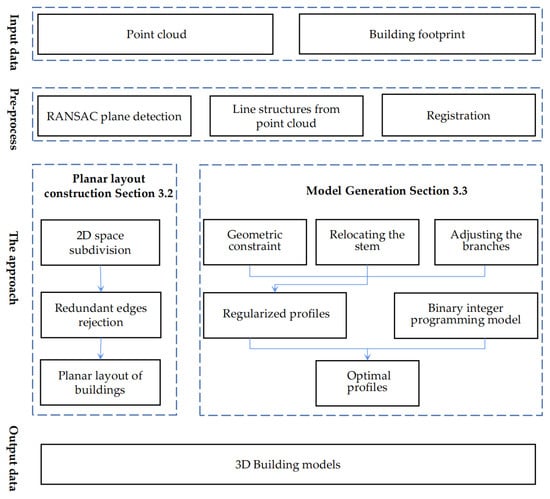
Figure 1. Workflow of the proposed building reconstruction method.

In the pre-processing steps, vertical planes are extracted from the point cloud using the RANSAC method [45] and then projected onto the XOY plane to generate the line structures of buildings. After that, the footprint data are introduced and aligned precisely with the point cloud in the XOY plane since the difference in source and representation between the two data types inevitably results in deviations in position. Using line features as primitives is the preferred alternative based on the representations of two data. Because of the difficulty of establishing the correspondences of a single line, we adopt the concept of line junctions. A line junction is a pair of intersecting lines, whereby the position of the intersection lies within a certain buffer of the segment. The principle for measuring the similarity of a pair of junctions is that their angular difference is less than a threshold and that the corresponding line segment projection distance is minimized when the junctions are aligned. For details of the pre-processing step, please refer to the work by [46].

Then, a two-stage reconstruction method is implemented. In the first stage, the planar layouts of buildings are constructed using footprint data and line structures of buildings generated from the point cloud. The edges are reoriented with reference to the footprint and screened based on spatial consistency.

In the second stage, for each edge in the planar layout, the façade points located on it are projected onto its vertical plane, producing a point density distribution. The optimal profile for each edge is then generated via clustering, regularization, and a binary integer programming function. Finally, the combination of the planar layout and the optimal profile generates a 2D topology to reconstruct the 3D model of the buildings.

3.2. Planar Layout Construction for Single Building

The planar layout consists of two parts. The exterior footprint represents the façade structure of the building, and the interior edges indicate the roof structure with a distinct altitude difference. First, the footprint of the building is labeled as BF, and the line segments inside the footprint range (R_BF) are selected, i.e., for l_k, if l_k∩R_BF ≠ l_k, l_k is rejected, and vice versa. Then, the interior line segments are extended to subdivide the footprint, and multiple auxiliary edges are obtained, as shown in Figure 2. However, due to the noise in the point cloud, line structures of the building extracted from the point cloud are unavoidably affected. Thus, the footprint data is employed as a reference. Considering the regularity in the footprint, such as perpendicularity and parallelism, we adjust the direction of the auxiliary edges.

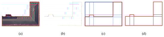
Figure 2. Illustration of the generation of auxiliary edges by combining the point cloud and footprint: (a) building point cloud and its footprint; (b) line structures of the building extracted from the point cloud; (c) the partition using interior line segments; (d) the red polygon denotes the footprint data, and the gray lines denote the auxiliary edges.

It is vital to select the valid edges to construct a building layout with the correct semantic rules. An illogical selection will cause errors in the topology of the final building models, such as self-intersections, internal overhangs, and non-closing edges. Thus, this paper designs an edge selection method based on spatial consistency. First, the BF is divided into multiple rectangles Sr by auxiliary edges, and each rectangular r_i ∈ Sr may represent a roof structure with a different height. To increase the robustness of the algorithm against point cloud noise, the average height of the point cloud located in r_i is used as the height of r_i, labeled as h(r_i). The flow of the method is as follows:

Calculate the distance d(e_k, e_k’) between the parallel edges e_k, e_k’ in rectangle r_i.

Calculate the height difference of edge e_k, hd(e_k), i.e., the height difference of between the two rectangles sharing edge e_k, $hd\left(e_k\right)=\parallel h\left(r_i\right)-h\left(r_i\right)\parallel$. Furthermore, if e_k ∈ BF, then $hd\left(e_k\right)=\parallel h\left(r_i\right)-0\parallel$.

Construct the optimization function for e_k. Footprint data carries accurate boundary and property information; therefore, any edge that lies on the footprint needs to be preserved. This means that only the edges interior to the footprint need to be handled. Constructing the objective function ensures that the optimal solution provides the optimum fitting to the point cloud. Equation (1) is used to determine whether e_k lies inside BF. Equation (2) is used to ensure that the selected edge possesses a height difference, where the weight α determines the details of the reconstructed roof; different weights are set according to the characteristics of different scenes. Considering the global structures, the optimization function is conducted in the form of Equation (3).

$$f1=\{\begin{array}{l}1,e_k not is BF edge\hfill \\ 0,e_k is BF edge\hfill \end{array}$$

(1)

$$f2=\alpha \ast x_e+hd\left(e_k\right)\ast \left(\neg x_e\right)$$

(2)

$$min{\displaystyle \sum }_{e_k}f1f2$$

(3)

where x_e ∈ {0, 1}, x_e = 0 indicates e_k is rejected, and x_e = 1 indicates e_k is preserved, as shown in Figure 3. A standard library, namely, the Gurobi Optimization [47], is used to solve these problems.

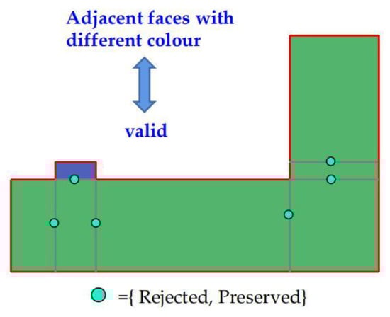
Figure 3. Illustration of the selection of valid edges.

3.3. Model Generation Based on 2D Topology of Building

The point cloud located on the edge is plotted into the same X-Z coordinate system, where X is perpendicular to the edge and extends inwards (positive) and outwards (negative) towards the building, and Z expresses the height vertically. The regularization of building structures can be presented quantitatively using the type of profiles. Guided by this idea, the profiles are first clustered and regularized to obtain an alternative profile set. An optimization function is then constructed to select a best-fit profile type for each e_k, thus constructing the 2D topology of the building.

3.3.1. Clustering and Regularization for Profiles

It would be challenging to parameterize the whole continuous façade structure lying on the edge e_k. As the profiles of e_k are all located within the same X-Z coordinate system, there are sure to be clusters of points, areas where the points are sparse, representing the location of noise, and areas where the points are denser—more likely a representative structure of the façade. Therefore, according to this feature, we choose the DBSCAN (Density-Based Spatial Clustering of Applications with Noise) algorithm [48], which is a representative density-based clustering algorithm with the ability to partition regions with sufficient density into clusters and to discover arbitrarily shaped clusters in the influence of noise. Firstly, the closeness of the sample distribution is portrayed by the neighborhood parameters (Dist, MinPts), with Dist denoting the neighborhood range and MinPts denoting the number of neighborhood points. In this study, the value of Dist is set to the resolution of the point cloud (r), and the value of MinPts is set to l(e_k)/(2r). When the number of neighborhood points within Dist exceeds MinPts, the points are taken as core points. Then, an arbitrary Point A is chosen, and according to the parameters, it is determined whether Point A is a core point. If so, the other Points B, C, D… within the Dist of Point A are traversed and identified as the same group, again to determine whether the Dist of Points B, C, D… contains other points that have not been traversed. If so, they are grouped with A. The previous step is repeated until all points are traversed and classified.

Monotonic profiles are preferred in the subsequent process. This paper introduces several regularity constraints to ensure the vertical and horizontal structure of the profile. A bottom-up strategy is used to gradually adjust the polyline segments obtained above. The specific strategy is as follows:

(1)

Eliminating the fragmented line segments. These fragmented line segments tend to be found at small parts on the surface of buildings, such as artifacts, chimneys, and dormers, so this paper stipulates that line segments less than 1 m in length are to be eliminated.

(2)

Determining and orienting the stem of polyline segments. The lengthiest vertical or near-vertical line segment is selected as the stem of the polyline segments and is reoriented to vertical, which can reduce the effects of occlusion, particularly in areas close to the ground.

(3)

Relocating the stem. The stem is extended to the ground, and its intersection with the ground must lie on edge e_k.

(4)

Adjusting the branches. The branches are extended to intersect with the stem, and nearly horizontal or vertical lines are snapped to the orientation.

(5)

If there is no vertical part of the profile on e_k, a vertical straight line segment is assigned to the profile, starting from the point located on e_k, and the rest of the lines are then connected to this vertical line.

3.3.2. Selecting Optimal Profile for Each Edge

Once the processing above is complete, each edge e_k corresponds to a set of regularized profiles, labeled as RP(e_k). An optimal profile needs to be chosen from the set RP(e_k). We assign to e_k a binary vector η(e_k) = {y₀, y₁, …, y_|P|}, y_i ∈ {0, 1}, whose dimension |P| is the number of types of profiles after clustering and regularization, as shown in Figure 4. Since only one profile type can be selected for edge e_k, the constraint Σ_iy_i = 1 is required. We use regularized profiles rp, rp ∈ RP(e_k), to fit the point clouds at the corresponding locations and then take the best-fitted profile as the optimum. Since the vertical part of the profile has been optimized in the above step, only the fitting of the profile branches to the point cloud is considered here. We use the point cloud O, which has been projected in the XOZ plane, as the fitted data and accumulate the distance f(e_k) from the point cloud to the profile branch. Ax + Bz + C = 0 is the linear equation coefficient of the profile branch.

$$f\left(e_k\right)={\displaystyle \sum }_{\left(x_i, z_i\right)\in \mathit{O}}\frac{A_k{x}_i+B_k{z}_i+C_k}{\sqrt{A_k^2+B_k^2}}$$

(4)

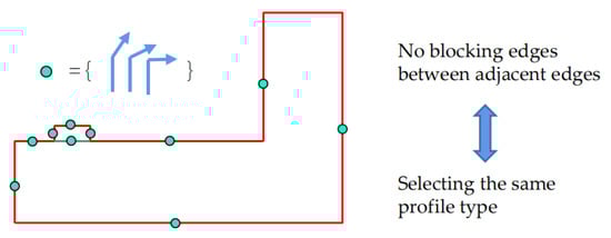
Figure 4. Illustration of the selection of profile types.

Finally, a global minimum energy function is constructed to select the optimal profile type for all edges in the same face. Equation (5) is a binary integer programming model, and the optimal solution can be solved using the Gurobi library to obtain the best configuration.

$$min{\displaystyle \sum }_{e_k}\frac{f\left(e_k\right)}{n\left(\mathit{O}\right)}·{\mathit{\eta }}_k$$

(5)

In addition, to take into account the regularity property, the set of edges ε = {e_i, e_j} that are approximately co-linear and have no blocking edges should have the same selection vector.

$$same\left({\mathit{\eta }}^i,{\mathit{\eta }}^j\right)=1,\forall \left(i,j\right)\in \epsilon$$

(6)

3.3.3. Construction of the 2D Topology

The 2D topology of a building is constructed as shown in Figure 5. Each edge e_k in Figure 5a corresponds to an optimal profile op_k. The profile can be divided into two parts, which we label as the stem part op_k(stem) and the branch part op_k(branch); θ is the horizontal angle of op_k(branch), as shown in Figure 5b. We found that by shifting these edges to a specific length and direction, as shown in Figure 5c, their intersecting trajectories could generate a 2D topology of the building, as shown in Figure 5d. The vector is perpendicular to the edge and its norm is op_k(branch)cos(θ). Considering the influence of noise, the normalization strategy is used here; the norm of the vector is cos(θ). We label this vector as the velocity vector of e_k.

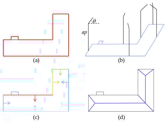
Figure 5. Illustration of the construction of the 2D topology. (a) the edges in a building; (b) the profiles corresponding to the edges; (c) the shifting of edges; (d) the 2D topology of the building.

For an arbitrary edge e_k, the direction of its intersection trajectory with its two neighboring edges can be calculated by the vector product of their velocity vectors. Since it is rare for four planes to intersect in a 3D surface space, the intersection of edges used in this paper is shown in Figure 6. First, the intersection line between e_k and its parallel edge is calculated, as shown with the blue line segment. Then, the intersection trajectories of the two ends of e_k are extended, as shown in the red and green line segments. Finally, the three line segments are used to make an intersection judgement. We define this intersection judgment as two cases. One is that the red and green line segments complete their intersection before intersecting the blue line segment, which then generates a vertex as shown in Figure 6a. The second is that the red and green line segments intersect the blue line segment separately, which then generates two vertices and a roofline as shown in Figure 6b. Once all the edges have been processed as described above, a 2D topology of the building can be generated.

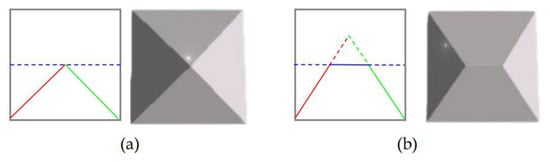
Figure 6. Illustration of edges intersection. (a) the intersection of two line segments; (b) the intersection of three line segments.

3.3.4. Three-Dimensional Building Model Reconstruction

The 3D building model will be constructed based on the 2D topology and the parameters of the optimal profiles. In our framework, each cell in the 2D topology represents a roof facet of the 3D building, and then the vertices of its boundaries can be accessed directly from the 2D topology. The z coordinate, the only unknown quantity, can be calculated from the profile to which the vertices belong.

4. Experiments

4.1. Datasets Descriptions

The experimental datasets are oblique photogrammetric point clouds and corresponding building footprints acquired in Shenzhen, China, and Dortmund, Germany [49]. For the point cloud in Shenzhen, the whole scene covers an area of 266,770 m² and is divided into four tiles (S1–S4), as shown in Figure 7. For the point cloud in Dortmund, the whole scene covers an area of 71,912 m² and is divided into two tiles (D1 and D2), as shown in Figure 8. The buildings footprint data of Shenzhen and Dortmund were obtained from Google Map and OSM, respectively. To ensure sufficient accuracy to meet the experimental requirements, the footprints need to be rectified manually in ArcGIS based on aerial images. The following is the specific procedure, we used the DOM with 8 cm resolution generated from the oblique images as base map to modify the footprint, mainly including the shape and position of the buildings’ boundary. An example is shown in Figure 9.

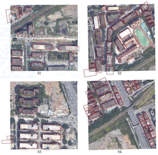
Figure 7. Four tiles of the photogrammetric point cloud and corresponding buildings footprint data (red polygons) in Shenzhen.

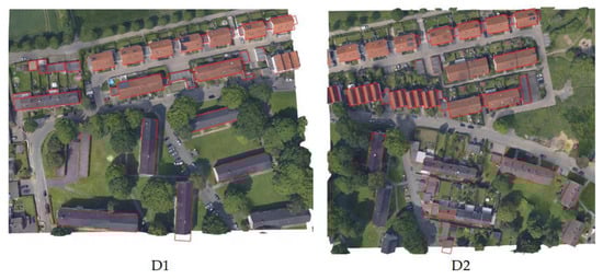
Figure 8. Two tiles of the photogrammetric point cloud and corresponding buildings footprint data (red polygons) in Dortmund.

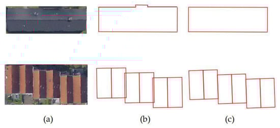
Figure 9. The example of the footprint modification: (a) DOM of buildings; (b) original footprint data; (c) modified footprint.

The point clouds are generated from images captured by an oblique photogrammetry system equipped with five cameras (one nadir and four oblique views). Table 1 lists the information of oblique images, and other parameters that are not described are unknown. With three known GCPs, seven known check points, and the position and attitude of the camera corresponding to each photo, existing solutions in Context Capture accomplish aerial triangulation (AT), and dense matching to generate photogrammetric point clouds. After AT, the global root mean square (RMS) of reprojection errors is 0.58 px, the global RMS of horizontal errors is 0.01 m, and the global RMS of vertical errors is 0.054 m for Shenzhen oblique images. The global RMS of reprojection errors is 0.6 px, the global RMS of horizontal errors is 0.017 m, and the global RMS of vertical errors is 0.065 m for Dortmund oblique images. Table 2 lists the basic information of the point clouds. To prove the effectiveness of our method, both qualitative and quantitative analyses were carried out, as shown below.

Table 1. Detailed information of the oblique images.

Region	Cameras	Calibration	Overlap (%) Forward/Side	GSD (cm) Nadir, Oblique
Shenzhen	Phase One IQ180	Lab	80/80 (all images)	8, 6–16
Dortmund	Hasselblad H3DII-50, Hasselblad H4D-50	Lab	75/80 (nadir images) 80/80 (oblique images)	10, 8–12

Table 2. Detailed information of the experimental point clouds.

Region	Datasets	Number of Points	Scene Area (m2)	Average Point Density (p/m3)	Average Point Distance (m)	Number of Buildings
Shenzhen	S1	9,544,816	67,077	102	0.05	14
	S2	11,086,652	68,121	102	0.04	30
	S3	10,192,762	65,278	103	0.04	9
	S4	9,805,454	66,294	102	0.05	33
Dortmund	D1	12,633,372	35,956	254	0.03	30
	D2	12,465,417	35,956	255	0.03	49

4.2. Qualitative Evaluations

First of all, the reconstructed models of all buildings are shown in Figure 10 and Figure 11. These scenes contain several typical areas. First, the complex structures of building boundaries and detailed structures are often smoothed out in oblique photogrammetry point clouds. Second, there are connectivity architectures between buildings, and building identification methods based on point-to-point connectivity usually discriminate such groups as one building, which is not conducive to subsequent building modeling. Third, the occlusion problem, mostly occurring when vegetation obscures the bottom of a building, results in noticeable distortions in the point cloud of the corresponding area. For these situations, we first introduce the building footprint as a constraint that can easily single out buildings, avoid topological errors in adherent buildings, and restrain building boundaries from recovering a more detailed structure. Then, using façade regularization, the distortion at the bottom of the building point cloud caused by shading from other buildings or vegetation is eliminated. At the same time, the missing parts of the façade are automatically filled in. The results show that the reconstructions are generally consistent with the appearance of the buildings in the point cloud, indicating the excellent performance of the proposed method.

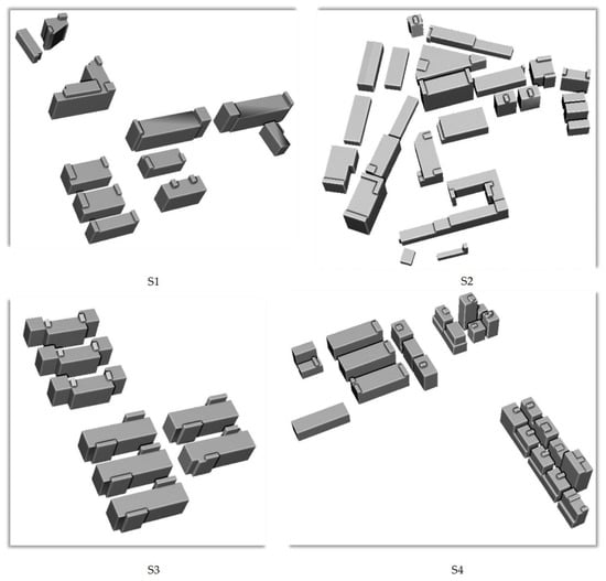
Figure 10. Reconstruction results of all buildings in Shenzhen.

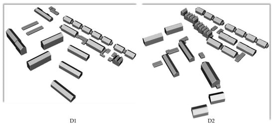
Figure 11. Reconstruction results of all buildings in Dortmund.

To further evaluate the proposed method, We chose nine buildings as experimental objects because they are universal and have different typical structures, including flat floors, multi-stories, and gable roofs, and the corresponding benchmarks were modeled manually in Sketchup, as shown in Figure 12, Figure 13, and Figure 14. Firstly, compared with the results of manual modeling, we can qualitatively state that our method performs well in modeling buildings with different architectural styles. Specifically, (1) it can adapt to different types of buildings, including flat floors and gable roofs; (2) the reconstructed models have the correct topology; and (3) the influence of artifacts can be reduced. However, some detailed structures will be missed, such as the parapets around the roof in Buildings 2–6 and the chimney in Buildings 7 and 8. Nevertheless, the overall reconstruction results can satisfy the LoD-2 level of detail.

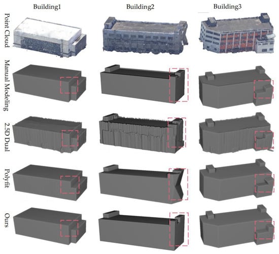
Figure 12. Comparison of models generated using the manual modeling, the 2.5D DC method, the PolyFit method, and our proposed method for Buildings 1, 2, and 3.

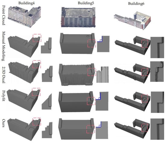
Figure 13. Comparison of models generated using the manual modeling, the 2.5D DC method, the PolyFit method, and our proposed method for Buildings 4, 5, and 6.

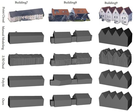
Figure 14. Comparison of models generated using the manual modeling, the 2.5D DC method, the PolyFit method, and our proposed method for Buildings 7, 8, and 9.

Then, contrastive analysis was performed using two state-of-the-art 3D building reconstruction methods, i.e., the 2.5D dual contouring method (2.5D DC) [50] and PolyFit [51]. All methods are successful in reconstructing building models from point clouds. The 2.5D DC method is a triangulated mesh modeling method. PolyFit and our method are structure modeling methods, meaning that 2.5D DC requires more facets than the other two methods to reconstruct the models. In addition, the 2.5D DC method enables the reconstruction of more detailed structures on the roof, such as Building 5, but is more susceptible to noise, such as Building 8, resulting in a coarser model. In contrast, the PolyFit method and our method are prominent in the reconstruction of buildings with regularity. The PolyFit method uses extracted planes to perform a 3D space subdivision, which generates thousands of candidate faces. With complete faces extracted, this method can generate good building models (Buildings 7 and 9). However, this process not only increases the high computational costs but is also highly susceptible to the quality of the plane segmentation. The main manifestations are as follows: (1) the extracted facets are severely affected by noise (Buildings 1 and 2); (2) adjacent facets are identified as the same facet (Buildings 4 and 6); and (3) vertical or horizontal facets are not extracted correctly (Buildings 3, 5, and 8). These can result in topological errors and regularization deficiencies in the final reconstructed model. Different from PolyFit, our proposed method uses only vertical or near-vertical planes, which excludes interference from other planes and dramatically reduces the effect of noise. In addition, we also use space subdivision but on a 2D plane, thus significantly reducing computational costs. Finally, in the façade abstraction and 2D topology construction, regularization constraints are introduced several times in this paper, so the final reconstructed model has a strong regularity.

4.3. Quantitative Evaluations

Firstly, to quantitatively evaluate the accuracy of the reconstructed results, we manually digitalized the whole buildings and took them as ground truth. We performed an overall assessment of the accuracy of the reconstructed building surfaces. Therefore, three indicators, namely, precision, recall [4], and F1 score were adopted to evaluate the accuracy of all reconstructed building models, as shown in Table 3. They are defined as:

$$\begin{array}{l}\mathrm{Precision}=\frac{\mathrm{TP}}{\mathrm{TP}+\mathrm{FP}}\hfill \\ \mathrm{Recall}=\frac{\mathrm{TP}}{\mathrm{TP}+\mathrm{FN}}\hfill \\ \mathrm{F}1\mathrm{Score}=2\times \frac{\mathrm{Precision}\times \mathrm{Recall}}{\mathrm{Preccision}+\mathrm{Recall}}\hfill \end{array}$$

(7)

where TP is the number of correctly reconstructed faces, FN is the number of faces in the ground truth that are not reconstructed, and FP is the number of reconstructed faces that are not found in the ground truth.

Table 3. Quantitative evaluation of reconstructed building surfaces.

Datasets	TP	FN	FP	Precision (%)	Recall (%)	F1 Score
S1	148	17	5	96.7	89.7	0.93
S2	223	34	7	97.0	86.8	0.92
S3	121	22	10	92.4	84.6	0.88
S4	240	59	22	91.6	80.3	0.86
D1	241	28	14	94.5	89.6	0.92
D2	344	72	22	94.0	82.7	0.88

According to Table 3, the precision values of all datasets are higher than 90%, the values of recall are greater than 80%, and the values of F1 score are greater than 0.86,which proves that the method in this paper can successfully reconstruct the building surface structure. In general, the high precision and low FP indicate that the reconstructed models have the correct topology. The data of S1–S4 are located in urban areas, where the buildings are tall, and their roofs are more complex. Some small details tend to be neglected in the reconstruction process, which leads to a high value of FN, especially in S4. Similarly, the data of D1 and D2 are located in the countryside, where the buildings are low, and these buildings with a low height and small area tend to be missed in the reconstruction process, especially in D2. Although there are cases where details are eliminated, the models reconstructed by our method can correctly represent the main structures of the buildings.

To further evaluate the proposed method, we calculated the distance between the point cloud and the model(C2M), as shown in Figure 15 and Figure 16. The C2M indicates the fitting degree between the point cloud and the model.

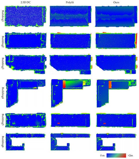
Figure 15. Evaluations of reconstructed Buildings 1–6 using the 2.5D DC, PolyFit, and the proposed method. The distance of the point cloud to the model is rendered with color.

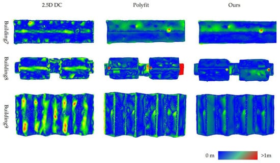
Figure 16. Evaluations of reconstructed Buildings 7–9 using the 2.5D DC, PolyFit, and the proposed method. The distance of the point cloud to the model is rendered with color.

For Buildings 1–6 generated by 2.5D DC, the C2M is rarely greater than 2 m, and the areas with significant distance differences are mostly distributed in the edge location. Meanwhile for Buildings 7–9, the C2M of 2.5D DC is mainly distributed between 0 and 1 m, and significant distance differences are mostly mainly located on the roof ridge. This verifies the above analysis that the method is severely affected by noise, especially in the edge areas. Additionally, since it is a triangular mesh reconstruction method, it can reconstruct the detailed parts. For PolyFit and the proposed method, the difference in results is not significant. For Buildings 1–6, the locations where the distance difference is greater than 2 m are generally distributed among point cloud distortions on the façade caused by occlusion. Note that the red area located on the roof of Building 4 is an un-reconstructed structure. Because the vertical planes adjacent to it were not successfully extracted, PolyFit could not form a closed cell, and our method could not construct a 2D topological cell. Another model with very significant differences is Building 2. The model generated by our method shows a large area of red at the right-hand façade, indicating a significant C2M in this area. A comparative analysis with the original point cloud reveals that the point cloud at this location shows large areas of severe distortion due to severe occlusion. If only to fit the point cloud, the generated model will come out with obvious topological errors, as shown in Figure 12. The proposed method uses footprint data with bespoke rule constraints to generate a reasonable building model. The results for Building 7 show little difference between our method and PolyFit. For Building 8, the area with a greater discrepancy is located on the right side of the building. Since the vertical plane of this part could not be extracted, the PolyFit method is unable to close this component, which in turn leads to the final model missing this part. Our method benefits from the boundary information provided by the footprint to recover the closed model. For Building 9, both methods do not produce large distance differences. The discrepancy is that the distance differences of PolyFit are mainly located on the ridge line, while those of our method are mainly located on the roof surface. This is because the optimization of PolyFit focuses on the fit of the plane, while the optimization of our method focuses on the regular direction of the profiles.

We then used the root mean square error (RSME) to measure the difference between the point cloud and the generated model, as shown in Equation (8). The results are shown in Figure 17.

$$RMSE=\sqrt{\frac{1}{N}{\displaystyle \sum }_{i\in N}\parallel p_i,M_b{\parallel }^2}$$

(8)

where N denotes the number of points in the building point cloud, and ||p_i, M_b|| denotes the Euclidean distance between point p_i and building model M_b.

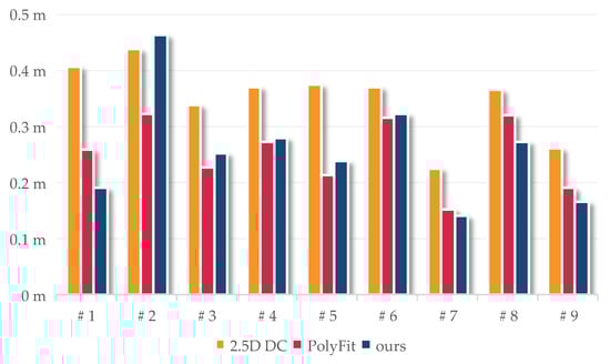
Figure 17. The RMSE_c2m of nine building models generated using 2.5D DC, PolyFit, and our proposed method.

For building models generated by 2.5D DC, the RMSE distribution ranges between 0.2 m and 0.5 m, which is larger than that of the other two methods, mainly because the façade of the building is not properly reconstructed. For building models generated by PolyFit and our method, their RMSEs are almost always at the same level, except for Buildings 1, 2, and 8. For Buildings 1 and 8, the RMSE error of the model reconstructed by PolyFit is significantly higher than that of the model reconstructed by our method. The Polyfit method generates the correct model, which requires identifying each planar structure and performing spatial subdivisions and selecting candidate facets. However, due to the existence of an unextracted façade, to generate a closed model, the Polyfit method will choose other neighboring planes to form a box, which in turn leads to the wrong structure of the model (Building 1), or it will choose to discard this structure when it cannot be combined with other neighboring planes to form a box, resulting in the absence of the structure in the final model (Building 8). Although the construction of the 2D topography in our method also requires vertical planes, structural errors at the façade rarely occur because of the footprint data as a supplement. On the contrary, for Building 2, the RMSE error of the model reconstructed by our method is significantly higher than that of the model reconstructed by the Polyfit method. The façade point cloud on the right side of Building 2 has adhesion with other objects, but some fragment planes can be extracted, so the model from the Polyfit method can fit this part point cloud. Our method uses the vertical rule of façade, so the model from our method does not completely fit this part point cloud.

Finally, the benchmark models were used to evaluate the building models generated from each method. We used RMSE_m2m to measure their difference, as shown in Figure 18. The smaller the RMSE_m2m value, the higher the model accuracy. Among all three methods, the RMSE_m2m of the 2.5D DC is the largest, and the RMSE_m2m of the proposed method is the lowest. It is worth noting that neither our method nor the Polyfit method recovered the overhang structure of Building 8, so the RMSE_m2m of the reconstructed model is larger. Compared with Figure 17, when RMSE_m2m is large and RMSE_c2m is small, it indicates that the reconstructed model does not fit the correct structure influenced by artifacts, such as Building 2 from the Polyfit method. When RMSE_m2m is small and RMSE_c2m is large, it indicates that the reconstructed model is not influenced by artifacts and recovers the correct structure, such as Building 2 of the proposed method. When RMSE_m2m is small and RMSE_c2m is small, it indicates that the reconstructed model is correct and fits the point cloud, such as Buildings 7 and 9 from the proposed method. The experiments prove that our reconstructed results have higher accuracy, strong regularity, and topological integrity and can be used as a data foundation to support higher-level detail model reconstructions.

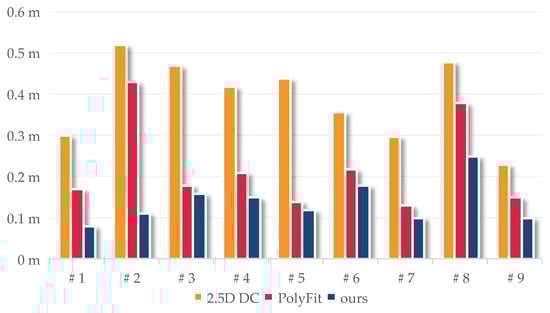
Figure 18. The RMSE_m2m of nine building models generated using 2.5D DC, PolyFit, and our proposed method.

5. Discussion and Limitations

The priority of the building reconstruction procedure is to complete the plane extraction. The plane extraction methods widely used in industrial applications include region growing and RANSAC-based methods. However, neither of these two methods can guarantee complete extraction. Both the Polyfit method and our approach use the RANSAC-based method. The former uses a strategy of spatial subdivision by extending the planes in 3D space to generate a closed model. Inspired by this, we use two-dimensional spatial subdivision to overcome the problem of incomplete plane extraction. Moreover, the complexity of subdivision in two dimensions is much lower than that in three dimensions. The problem of incorrect segmentation can cause topological errors in the reconstructed model. The Polyfit method uses manual interaction to add missing planes and lacks an effective means to correct planes with incorrect orientation. We introduce footprint data as a supplement and shape constraint to alleviate and avoid these problems. In addition to the façade, the roofs of our reconstructed buildings have strong regularity. The Polyfit method focuses on fit and closure, while our method adds regularity. Thus, the reconstructed models from the Polyfit method are closer to the point cloud for some buildings, resulting in lower RMSE_c2m than those of our approach. However, the Polyfit method is more susceptible to the influence of artifacts, which reduces the quality of reconstructed models.

In this paper, experiments were conducted using an oblique photogrammetric point cloud and footprint from two regions. The characteristics of the proposed method and its possible limitations are discussed below. The experiments show that, overall, the precision value of the reconstructed models using our method is higher than 90%, the value of recall is higher than 80%, and the values of F1 score are greater than 0.86. Additionally, the reconstructed models using our method have stronger regularity than those of the other methods. While using oblique photogrammetric point clouds for modeling, two data quality challenges need to be addressed: one is smoothed sharp features, and the other is data distortion. The former are mostly located at the edges of planes, while the latter is mostly located at façades or planes with occlusion. Our method adopts the strategy of abstracting the façade by using a monotonically regular profile to parameterize the façade structure, such as Building 2 and Building 9. In this process, this method focuses on the optimization of the main orientation, with the advantage that the main structure of the building can be concisely recovered, and the disadvantage is that it is difficult to avoid smoothing out some detailed parts. Therefore, the result generally has more un-reconstructed facets than incorrectly reconstructed facets. In addition, to restore the correct topological relationship, our method constructs the topology in two dimensions. This makes it easier to establish regular spatial relationships such as perpendicular, parallel, and symmetrical relationships, which enables the reconstruction of buildings with excellent regularity. However, there are some limitations. This paper uses a bottom-up reconstruction strategy. The 3D model is obtained by pulling up the 2D topology. This manner prevents us from generating models with suspended structures. Moreover, the basis for performing the regularization is the ability to accurately determine the main orientation of the building in two dimensions and use it as a reference, so this paper requires the introduction of the building footprint, which leads to the dependence of our method on the accuracy of the data. In view of the fact that the production of high-precision footprints has been developed for decades, they are sufficient as constrained data for the 3D reconstruction of buildings. Therefore, the method proposed in this paper can provide a feasible technical solution for large-scale automated production of 3D city models.

References

- Gröger, G.; Plümer, L. CityGML—Interoperable semantic 3D city models. ISPRS J. Photogramm. Remote Sens. 2012, 71, 12–33. [Google Scholar] [CrossRef]
- Verdie, Y.; Lafarge, F.; Alliez, P. LOD Generation for Urban Scenes. ACM Trans. Graph. 2015, 34, 30. [Google Scholar] [CrossRef]
- Xu, B.; Hu, H.; Zhu, Q.; Ge, X.; Jin, Y.; Yu, H.; Zhong, R. Efficient interactions for reconstructing complex buildings via joint photometric and geometric saliency segmentation. ISPRS J. Photogramm. Remote Sens. 2021, 175, 416–430. [Google Scholar] [CrossRef]
- Li, L.; Song, N.; Sun, F.; Liu, X.; Wang, R.; Yao, J.; Cao, S. Point2Roof: End-to-end 3D building roof modeling from airborne LiDAR point clouds. ISPRS J. Photogramm. Remote Sens. 2022, 193, 17–28. [Google Scholar] [CrossRef]
- Awrangjeb, M.; Gilani, S.; Siddiqui, F. An Effective Data-Driven Method for 3-D Building Roof Reconstruction and Robust Change Detection. Remote Sens. 2018, 10, 1512. [Google Scholar] [CrossRef]
- Li, Y.; Wu, B. Relation-Constrained 3D Reconstruction of Buildings in Metropolitan Areas from Photogrammetric Point Clouds. Remote Sens. 2021, 13, 129. [Google Scholar] [CrossRef]
- Zhou, G.; Zhou, X.; Song, Y.; Xie, D.; Wang, L.; Yan, G.; Hu, M.; Liu, B.; Shang, W.; Gong, C.; et al. Design of supercontinuum laser hyperspectral light detection and ranging (LiDAR) (SCLaHS LiDAR). Int. J. Remote Sens. 2021, 42, 3731–3755. [Google Scholar] [CrossRef]
- Hu, H.C.; Zhou, G.Q.; Zhou, X.; Tan, Y.Z.; Wei, J.D. Design and Implement of a Conical Airborne LIDAR Scanning System. Int. Arch. Photogramm. Remote Sens. Spat. Inf. Sci. 2020, XLII-3/W10, 1247–1252. [Google Scholar] [CrossRef]
- Chen, D.; Zhang, L.; Mathiopoulos, P.T.; Huang, X. A Methodology for Automated Segmentation and Reconstruction of Urban 3-D Buildings from ALS Point Clouds. IEEE J.-Stars 2014, 7, 4199–4217. [Google Scholar] [CrossRef]
- Li, M.; Rottensteiner, F.; Heipke, C. Modelling of buildings from aerial LiDAR point clouds using TINs and label maps. ISPRS J. Photogramm. Remote Sens. 2019, 154, 127–138. [Google Scholar] [CrossRef]
- Lin, L.; Yu, K.; Yao, X.; Deng, Y.; Hao, Z.; Chen, Y.; Wu, N.; Liu, J. UAV based estimation of forest leaf area index (LAI) through oblique photogrammetry. Remote Sens. 2021, 13, 803. [Google Scholar] [CrossRef]
- Zhang, Z.; Gerke, M.; Vosselman, G.; Yang, M.Y. A patch-based method for the evaluation of dense image matching quality. Int. J. Appl. Earth Obs. 2018, 70, 25–34. [Google Scholar] [CrossRef]
- Pan, Y.; Yiqing, D.; Wang, D.; Chen, A.; Ye, Z. Three-Dimensional Reconstruction of Structural Surface Model of Heritage Bridges Using UAV-Based Photogrammetric Point Clouds. Remote Sens. 2019, 11, 1204. [Google Scholar] [CrossRef]
- Biljecki, F.; Ledoux, H.; Stoter, J. An improved LOD specification for 3D building models. Comput. Environ. Urban Syst. 2016, 59, 25–37. [Google Scholar] [CrossRef]
- Krafczek, M.; Jabari, S. Generating LOD2 city models using a hybrid-driven approach: A case study for New Brunswick urban environment. Geomatica 2022, 75, 130–147. [Google Scholar]
- Yu, D.; Ji, S.; Liu, J.; Wei, S. Automatic 3D building reconstruction from multi-view aerial images with deep learning. ISPRS J. Photogramm. Remote Sens. 2021, 171, 155–170. [Google Scholar] [CrossRef]
- Widyaningrum, E.; Gorte, B.; Lindenbergh, R. Automatic Building Outline Extraction from ALS Point Clouds by Ordered Points Aided Hough Transform. Remote Sens. 2019, 11, 1727. [Google Scholar] [CrossRef]
- Özdemir, E.; Remondino, F.; Golkar, A. An Efficient and General Framework for Aerial Point Cloud Classification in Urban Scenarios. Remote Sens. 2021, 13, 1985. [Google Scholar] [CrossRef]
- Chen, M.; Feng, A.; McCullough, K.; Prasad, P.B.; McAlinden, R.; Soibelman, L. 3D Photogrammetry Point Cloud Segmentation Using a Model Ensembling Framework. J. Comput. Civ. Eng. 2020, 34, 4020048. [Google Scholar] [CrossRef]
- Chen, D.; Li, J.; Di, S.; Peethambaran, J.; Xiang, G.; Wan, L.; Li, X. Critical Points Extraction from Building Façades by Analyzing Gradient Structure Tensor. Remote Sens. 2021, 13, 3146. [Google Scholar] [CrossRef]
- Xu, Y.; Stilla, U. Toward Building and Civil Infrastructure Reconstruction From Point Clouds: A Review on Data and Key Techniques. IEEE J.-Stars 2021, 14, 2857–2885. [Google Scholar] [CrossRef]
- Ham, H.; Wesley, J.; Hendra, H. Computer vision based 3D reconstruction: A review. Int. J. Electr. Comput. Eng. 2019, 9, 2394. [Google Scholar] [CrossRef]
- Schwarz, M.; Müller, P. Advanced procedural modeling of architecture. ACM Trans. Graph. (TOG) 2015, 34, 1–12. [Google Scholar] [CrossRef]
- Saxena, A.; Sun, M.; Ng, A.Y. Make3D: Learning 3D Scene Structure from a Single Still Image. IEEE Trans. Pattern Anal. 2009, 31, 824–840. [Google Scholar] [CrossRef] [PubMed]
- Plyer, A.; Le Besnerais, G.; Champagnat, F. Massively parallel Lucas Kanade optical flow for real-time video processing applications. J. Real-Time Image Process. 2016, 11, 713–730. [Google Scholar] [CrossRef]
- Li, Z.; Shan, J. RANSAC-based multi primitive building reconstruction from 3D point clouds. ISPRS J. Photogramm. Remote Sens. 2022, 185, 247–260. [Google Scholar] [CrossRef]
- Jiang, Q.; Feng, X.; Gong, Y.; Song, L.; Ran, S.; Cui, J. Reverse modelling of natural rock joints using 3D scanning and 3D printing. Comput. Geotech. 2016, 73, 210–220. [Google Scholar] [CrossRef]
- Buonamici, F.; Carfagni, M.; Furferi, R.; Governi, L.; Lapini, A.; Volpe, Y. Reverse engineering modeling methods and tools: A survey. Comput.-Aided Des. Appl. 2018, 15, 443–464. [Google Scholar] [CrossRef]
- Wang, R.; Peethambaran, J.; Chen, D. LiDAR Point Clouds to 3-D Urban Models: A Review. IEEE J.-Stars 2018, 11, 606–627. [Google Scholar] [CrossRef]
- Huang, H.; Brenner, C.; Sester, M. A generative statistical approach to automatic 3D building roof reconstruction from laser scanning data. ISPRS J. Photogramm. Remote Sens. 2013, 79, 29–43. [Google Scholar] [CrossRef]
- Jarząbek-Rychard, M.; Borkowski, A. 3D building reconstruction from ALS data using unambiguous decomposition into elementary structures. ISPRS J. Photogramm. Remote Sens. 2016, 118, 1–12. [Google Scholar] [CrossRef]
- Buyukdemircioglu, M.; Can, R.; Kocaman, S. Deep Learning Based Roof Type Classification Using Very High Resolution Aerial Imagery. Int. Arch. Photogramm. Remote Sens. Spat. Inf. Sci. 2021, XLIII-B3-2021, 55–60. [Google Scholar] [CrossRef]
- Kada, M.; McKinley, L. 3D building reconstruction from LiDAR based on a cell decomposition approach. Int. Arch. Photogramm. Remote Sens. Spat. Inf. Sci. 2009, 38, 47–52. [Google Scholar]
- Zhu, Q.; Wang, F.; Hu, H.; Ding, Y.; Xie, J.; Wang, W.; Zhong, R. Intact planar abstraction of buildings via global normal refinement from noisy oblique photogrammetric point clouds. ISPRS Int. J. Geo-Inf. 2018, 7, 431. [Google Scholar] [CrossRef]
- Zhang, K.; Yan, J.; Chen, S. Automatic construction of building footprints from airborne LIDAR data. IEEE Trans. Geosci. Remote 2006, 44, 2523–2533. [Google Scholar] [CrossRef]
- Zhou, Q.; Neumann, U. Fast and Extensible Building Modeling from Airborne LiDAR Data. In Proceedings of the 16th ACM SIGSPATIAL International Conference on Advances in Geographic Information Systems; ACM: New York, NY, USA, 2008; p. 7. [Google Scholar]
- Poullis, C. A Framework for Automatic Modeling from Point Cloud Data. IEEE Trans. Pattern Anal. 2013, 35, 2563–2575. [Google Scholar] [CrossRef] [PubMed]
- Kelly, T.; Femiani, J.; Wonka, P.; Mitra, N.J. BigSUR: Large-scale structured urban reconstruction. Acm Trans. Graph. 2017, 36, 204. [Google Scholar] [CrossRef]
- Zhou, Q.; Neumann, U. 2.5 D building modeling by discovering global regularities. In Proceedings of the 2012 IEEE Conference on Computer Vision and Pattern Recognition, Providence, RI, USA, 16–21 June 2012; pp. 326–333. [Google Scholar]
- Xie, L.; Hu, H.; Zhu, Q.; Li, X.; Tang, S.; Li, Y.; Guo, R.; Zhang, Y.; Wang, W. Combined rule-based and hypothesis-based method for building model reconstruction from photogrammetric point clouds. Remote Sens. 2021, 13, 1107. [Google Scholar] [CrossRef]
- Verma, V.; Kumar, R.; Hsu, S. 3D Building Detection and Modeling from Aerial LIDAR Data. In Proceedings of the 2006 IEEE Computer Society Conference on Computer Vision and Pattern Recognition (CVPR’06), New York, NY, USA, 17–22 June 2006; pp. 2213–2220. [Google Scholar]
- Elberink, S.J.O. Target graph matching for building reconstruction. In Proceedings of Laser Scanning ’09; ISPRS: Paris, France, 2009; pp. 49–54. [Google Scholar]
- Xiong, B.; Elberink, S.O.; Vosselman, G. A graph edit dictionary for correcting errors in roof topology graphs reconstructed from point clouds. ISPRS J. Photogramm. Remote Sens. 2014, 93, 227–242. [Google Scholar] [CrossRef]
- Xu, B.; Jiang, W.; Li, L. HRTT: A Hierarchical Roof Topology Structure for Robust Building Roof Reconstruction from Point Clouds. Remote Sens. 2017, 9, 354. [Google Scholar] [CrossRef]
- Schnabel, R.; Wahl, R.; Klein, R. Efficient RANSAC for point-cloud shape detection. Comput. Graph. Forum. 2007, 26, 214–226. [Google Scholar] [CrossRef]
- Wang, F.; Hu, H.; Ge, X.; Xu, B.; Zhong, R.; Ding, Y.; Xie, X.; Zhu, Q. Multientity Registration of Point Clouds for Dynamic Objects on Complex Floating Platform Using Object Silhouettes. IEEE Trans. Geosci. Remote Sens. 2021, 59, 769–783. [Google Scholar] [CrossRef]
- Optimization, G. Gurobi Optimizer 9.5. Available online: www.gurobi.com (accessed on 12 May 2022).
- Schubert, E.; Sander, J.; Ester, M.; Kriegel, H.P.; Xu, X. DBSCAN revisited, revisited: Why and how you should (still) use DBSCAN. ACM Trans. Database Syst. (TODS) 2017, 42, 1–21. [Google Scholar] [CrossRef]
- Nex, F.; Gerke, M.; Remondino, F.; Przybilla, H.J.; Aumker, M.B.; Zurhorst, A. Isprs benchmark for multi-platform photogrammetry. ISPRS Ann. Photogramm. Remote Sens. Spat. Inf. Sci. 2015, II-3/W4, 135–142. [Google Scholar] [CrossRef]
- Zhou, Q.; Neumann, U. 2.5D Dual Contouring: A Robust Approach to Creating Building Models from Aerial LiDAR Point Clouds. In European Conference on Computer Vision, Computer Vision—ECCV 2010; Springer: Berlin/Heidelberg, Germany, 2010; pp. 115–128. [Google Scholar]
- Nan, L.; Wonka, P. PolyFit: Polygonal Surface Reconstruction from Point Clouds. In Proceedings of the IEEE International Conference on Computer Vision (ICCV), Venice, Italy, 22–29 October 2017; pp. 2353–2361. [Google Scholar]
Disclaimer/Publisher’s Note: The statements, opinions and data contained in all publications are solely those of the individual author(s) and contributor(s) and not of MDPI and/or the editor(s). MDPI and/or the editor(s) disclaim responsibility for any injury to people or property resulting from any ideas, methods, instructions or products referred to in the content. |
© 2023 by the authors. Licensee MDPI, Basel, Switzerland. This article is an open access article distributed under the terms and conditions of the Creative Commons Attribution (CC BY) license (https://creativecommons.org/licenses/by/4.0/).