Abstract
Glaciers are generally believed to be subjugating by global warming but the Karakoram glaciers are reportedly maintaining their balance. Earlier studies in the Karakoram and its sub-basins have mostly addressed a short span of time and used complex models to understand the phenomenon. Thus, this study is based on a long-term trend analysis of the computed runoff components using satellite data with continuous spatial and temporal coverage incorporated into a simple degree day Snowmelt Runoff Model (SRM). The trends of melt runoff components can help us understanding the future scenarios of the glaciers in the study area. The SRM was calibrated against the recorded river flows in the Hunza River Basin (HRB). Our simulations showed that runoff contribution from rain, snow, and glaciers are 14.4%, 34.2%, and 51.4%, respectively during 1995–2010. The melting during the summer has slightly increased, suggesting overall but modest glacier mass loss which consistent with a few recent studies. The annual stream flows showed a rising trend during the 1995–2010 period, while, rainfall and temperatures showed contrasting increasing/decreasing behavior in the July, August, and September months during the same period. The average decreasing temperatures (0.08 °C per annum) in July, August, and September makes it challenging and unclear to explain the reason for this rising trend of runoff but a rise in precipitation in the same months affirms the rise in basin flows. At times, the warmer rainwater over the snow and glacier surfaces also contributed to excessive melting. Moreover, the uncertainties in the recorded hydrological, meteorological, and remote sensing data due to low temporal and spatial resolution also portrayed contrasting results. Gradual climate change in the HRB can affect river flows in the near future, requiring effective water resource management to mitigate any adverse impacts. This study shows that assessment of long-term runoff components can be a good alternative to detect changes in melting glaciers with minimal field observations.
1. Introduction
The increase in global population during the past century up to 6 billion caused a six-fold increase in the demand for freshwater [1]. The fresh water demand is further projected to increase by 20% to 30%, i.e., from about 4600 km3 per year to 5500 to 6000 km3 per year, by 2050 [2]. With glaciers being perennial ice features that store fresh water, the fate of glaciers and sustainability of downstream fresh water availability are critically linked [3]. Climate change has been seriously affecting water resources since 1850 by increasing glacier melting across the globe [4,5,6,7,8]. This loss of glacier mass will affect the future availability of fresh water downstream [9], with serious consequences for dependent populations [10,11,12,13]. Furthermore, depletion of mountain glaciers have accounted for approximately 15–20% of the global sea level rise during the second half of the 20th century [14], and alarming forecasts of sea level rises of 5–17 cm [15,16] by the end of the 21st century. Furthermore, excessive melting along with other factors has caused massive rock and ice avalanches in the past [15], which very recently at Chamoli, Indian Himalaya in February 2021, turning into a disaster by killing 200 people and causing collateral damages [17]. Enhanced solar absorption by dust on snow and glacier surfaces causes excessive melting [18,19]. Glaciers are studied worldwide using satellite data (both optical and SAR) and derived products for their extent/volume quantification/glacier surface velocities [20,21], but sometimes they may give deceiving signals due to uncertainties in measurements and interpretation [22].
Glacier melt water in Hindukush, Karakoram, and Himalaya (HKH) mountain ranges has proven to be the major source of river flows, besides seasonal snow melt and rainfall runoff [23]. The entire Indus Basin is likely to be the most susceptible basin in the Hindukush–Karakoram–Himalaya (HKH) region to a reduction in river flows after the 2050s [23]. The yearly flow of the entire Indus River Basin (IRB) is more than 65% from snowfields, especially those which are above 3500 m in altitude [24,25,26,27,28,29]. The basin upstream of the Tarbela dam in Pakistan is generally referred to as the Upper Indus Basin (UIB) [24]. Archer et al. [30] used long-term stream flow data from nineteen low-altitude stations, to scrutinize the annual and seasonal flows in the UIB. Summer runoff in the UIB was closely correlated with the mean summer temperature causing melting of snow and glaciers [30]. Glaciers in the UIB cover approximately 17–22% of the High Mountain Asian region [31,32] and their melt water, therefore, makes an important contribution to the hydrology of the basin, providing 40% of the total downstream runoff [33]. Climate change is expected to alter the agro-climatic zones, ultimately reducing water availability [23,34,35,36,37].
The Karakoram Mountains alone accommodate 70% of the glaciers in the UIB [38]. The glaciers in Karakoram are considered to be stable [5,39,40,41,42,43] in the context of “Karakoram Anomaly” and are out of phase with global warming. The Hunza River Basin (HRB) is one of the most densely glacierized sub-basins of the UIB, situated in the western Karakoram mountain ranges. The current impact of climate change on the HRB glaciers is quite uncertain because of the scarcity of ground-based data—especially from higher altitudes, the low quality of the available observational data, and the low spatial and temporal resolution of the remote sensing data for cryospheric mapping.
Earlier investigations [31,44,45,46,47,48,49] have used optical/SAR remote sensing data and digital elevation models to estimate the extent as well as altitudinal changes in the glaciers within the basin. Few research studies [20,21] have utilized optical/SAR data for estimation of glacier surface velocities and their temporal variation. Others [24,50,51,52] have used temperature, precipitation, and river flow recordings for finding trends and determining their usefulness in snowmelt runoff modelling. They observed an increase in precipitation, a slight cooling in the summer, and a slight warming in the winter and spring, but nothing was statistically significant, as per their analysis. The glaciers in this area have been reported to be retreating by 1.36% on average during 1973 and 2015 [45], and are considered relatively stable compared to those in the Hindukush and Trans-Himalaya regions [31]. However, some observations [46,48] on selected glaciers in the HRB suggest a significant (7.6% of the glaciers area) retreat during the 1977–2014 period. A reduction in summer runoff (i.e., in melt runoff) was reported between 1967 and 2005 in Indus at Besham [50]. The evaluation of long-term changes to glaciers is challenging due to the shortage of mass balance studies and limited observation data [53]. Mass balance studies for glaciers in the Hunza River Basin mostly reported a stable or nearly stable situation during the 1970–2016 period [32,54,55], besides observed surface lowering and slightly negative mass balances of a few individual glaciers [55]. These studies were mostly based on only two-times satellite/geodetic data and thus lacked in providing a clearer picture of long-term continuous and annual variations.
Mass balance studies [32,54,55], with the help of extensive fieldwork, can provide authentic information of volume and mass changes. The rugged terrain of mountain glaciers, however, is the main hurdle to conduct field work thus making field data unavailable most of the time. Alternative methods are, therefore, must be explored to understand the fate of glaciers and hence, the climate in the region. Long-term annual variations in the runoff components to river flows can reflect climatic variations, a correlation that may be useful to know the volume changes in the glaciers and for future water resource management.
This study was conducted with the objective of assessing the glaciers’ health through long-term trend analysis of annual melt-runoff components. Trend analysis can be performed using either physically based distributed models or simple degree day models. The hydrological models based on the physical parameters require extensive input variables during calibration, which is extremely difficult in mountainous regions, particularly in Asia. Therefore, we used a degree day Snowmelt Runoff Model (SRM) to quantify the rainfall, snowmelt, and glacier-melt runoff. Satellite remote sensing data was used for quantifying the snow cover fraction, which was an important input to the SRM. The output simulations, meteorological data, and hydrological data were analyzed to assess the glacial status and climate trends in the basin.
2. Study Region and Meteorological Conditions
The HRB is situated in the western Karakoram range of Pakistan between longitudes 74.02°E and 75.78°E, and between latitudes 35.93°N and 37.09°N, covering an area of 13,876 square kilometers. The basin hosts Batura and Hispar glaciers that are more than 50 km long and are among seven longest glaciers in the world outside the polar regions. The hypsometric mean elevation of the basin is 4641 m above sea level (m.a.s.l.). The basin boundary is defined by the location of the stream gauge (here we call it the pour point). The catchment area and hypsometric mean elevation depend on the pour point selected. Therefore, our figure (13,876 sq km) for the Hunza Basin may differ from those of other investigations. The glacierized area is 4262 km2 according to the Randolph Glacier Inventory Version 6.0 (RGI 6.0), and 4053 km2 according to an estimate by [31], which is almost 30% of the HRB. The equilibrium line altitude (ELA) in the Hunza Basin has been estimated to be between 4500 m and 5500 m.a.s.l. [42,45,56,57,58,59].
The westerly circulations have a significant impact on the climate of the Karakoram region, with the winter and spring months receiving the most precipitation [28] and the summer months receiving the least amount of precipitation due to weak monsoonal incursions [60]. The mean annual precipitations recorded over sixteen years (1995–2010) at the Naltar, Ziarat, and Khunjerab meteorological stations were 680 mm, 225 mm, and 170 mm, respectively. Similarly, the mean annual temperatures at the Naltar, Ziarat, and Khunjerab meteorological stations were 6.4 °C, 2.6 °C, and −5.5 °C during the same period. The area covered under the snow in the study area fluctuates from 30% in summer to greater than 80% in winter [24]. The HRB contains six or seven sub-basins, making it too complex to be adequately represented by observations from just three stations, especially when all three of them are located in valleys. Figure 1 provides the locations of the meteorological and hydrological stations in the Hunza River Basin.
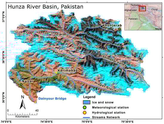
Figure 1.
Study area in northern Pakistan, representing the streams, valleys, and locations of the meteorological and hydrological stations.
3. Data Sets and Methods
3.1. Digital Elevation Models (DEM) Data
The DEM data derived from the Shuttle Radar Topography Mission (SRTM) was downloaded from www.earthexplorer.usgs.gov (accessed on 12 June 2022). The DEM, with a spatial resolution of 1 arc-second (equivalent to 30 m), was used to extract the basin characteristics, i.e., basin outline (boundary), elevation zones, and zonal hypsometric mean elevation required for the SRM. The Hunza basin was divided into 8 elevation zones, at intervals of 800 m (Figure 2b). The DEM was also used to extract zonal snow cover area, the total basin area, drainage network, and reference elevation of the basin outlet (River Gauge Station) as shown in Figure 2.
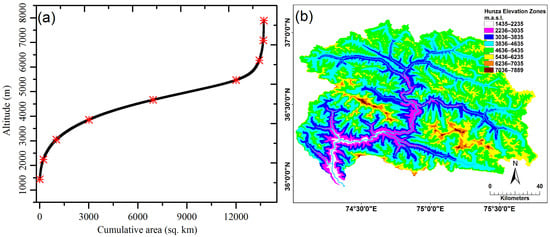
Figure 2.
(a) Cumulative area vs. elevation curve used for hypsometric mean elevations within the study area (red asterisks represent boundaries among elevation zones). (b) Hunza basin elevation zones and the drainage network.
3.2. Hydrological and Meteorological Data
The hydrological data of Pakistan was acquired from the Water and Power Development Authority (WAPDA) recorded under the Surface Water Hydrology Project (SWHP). Daily average river flows (in cubic meters per second) recorded at the Dainyour Bridge on the Hunza River during the 1966–2010 period were used in this study. Unfortunately, hydrological data was not available for the years 1999, 2005, 2006, and 2007. The recession coefficient (k) is vital for the SRM because (1-k) is the fraction of the daily melt-water that appears instantly in the runoff [61]. The available observational data was used to estimate the historical flow trends and calculate the recession coefficient (k). The observational hydrological data was used as an input to the model as well to assess the performance of the model by comparing the simulated runoff with the observed runoff.
The meteorological data was also acquired through the WAPDA Surface Water Hydrology Project (SWHP). The data from the Naltar (2810 m.a.s.l.), Ziarat (3669 m.a.s.l.), and Khunjerab (4730 m.a.s.l.) stations covered the period from 1995 to 2010. In addition to daily precipitation data, daily minimum and maximum temperatures were also used as input into the degree day SRM. Figure 3 represents the hydrological and meteorological observations during the respective periods.
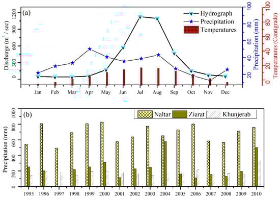
Figure 3.
(a) Monthly average discharge (m3/s), total precipitation (mm), and average temperature (°C) data for Hunza River Basin during the 1966–2010 period. (b) Total annual precipitation recorded at the three meteorological stations (Naltar, Ziarat, and Khunjerab) in Hunza Basin during the 1995–2010 period.
3.3. Remote Sensing of Snow Cover
Satellite data has been used for extracting snow cover extent in the different elevation zones, which was an important input for the SRM. There is no need to discriminate between snow and glacier, rather, snow and glacier are collectively taken as the “snow fraction” used in the SRM as input. However, such discrimination is possible in several ways. One way is to mask snow cover based on glacier outlines. Depending upon the time (season) and space (altitude) of the image pixels representing snow in a particular zone, relevant degree day factor values can be selected to simulate the runoff. Images stacked in a 7-2-1 (as RGB) band combination, with a 250 m spatial resolution (most of the studies have used comparatively low resolution data of 500 m) from the Moderate Resolution Imaging Spectro-radiometer (MODIS) sensors on the Terra and Aqua satellites, were downloaded from the NASA Worldview Snapshots website https://wvs.earthdata.nasa.gov/ (accessed on 1 February 2022). These images were processed and classified into snow and snow-free areas using supervised classification. Even though daily images were available from both these satellites, getting cloud-free images was not always possible. Snow-covered areas on cloudy days were therefore calculated using a linear interpolation technique between images from cloud-free days. It is important to mention that uncertainties in satellite-based snow cover, due to mixing of snow pixels in areas of forest cover or vegetation cover [62], requires careful evaluation to map snow cover in forested areas. The processing of snow cover raster data using DEM resulted in the snow fraction for each elevation zone. MODIS data was available for the period 2000–2010, whereas for the years earlier to 2000 (i.e., for 1995–1999), cloud-free higher spatial resolution Landsat images were used to determine the snow cover. Available cloud-free Landsat images were also used to modify the average snow depletion curves obtained from the Terra and Aqua satellite data for 2000–2010, which were then referred to as modified depletion curves, and these were used as input to the SRM for the period from 1995 to 1999. The SRM needs daily snow input which is possible only by daily passes of the Terra and Aqua satellites. Although high resolution Landsat data is available during 2001–2010, the acquisition of cloud-free images as well as daily temporal coverage (due to temporal resolution of 16 days) was not possible. Similarly, geo-stationary satellite imagery have been utilized [63] to estimate the snow cover, but the Hunza basin is relatively small and the resolution of such imagery was too coarse for this purpose in the basin. SAR data can be utilized to discriminate between wet and dry snow [64], but further classification of snow classes into wet and dry snow was also not the primary scope of this study. Therefore, MODIS images were mostly utilized for snow cover extraction in this study.
It is important to note that most of the seasonal snow is melted by June, except at higher elevation zones (Figure 4). In contrast, the hydrographs show increased river flows in July and August, indicating the increased proportion of ice melting that is mostly from glaciers in these months. This fact supports the reasoning for higher proportions of glacier melt in river runoff.
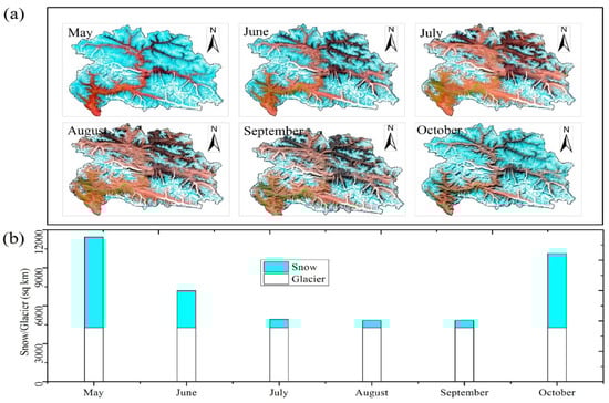
Figure 4.
(a) Monthly images acquired by MODIS sensors on the Terra and Aqua satellites, superimposed with glacier outlines. (b) Monthly snow cover (derived from satellite data shown in cyan color) variations vs. glacier cover shown in white (RGI 6.0) within the Hunza Basin.
3.4. Methods
The Snowmelt Runoff Model (SRM) was used to simulate the daily runoff contributions to river flows, compared to the observational discharge data (Figure 3). Satellite-based snow cover fractions were integrated with the SRM for runoff estimation. Chronological calibration, validation, simulation, and statistical analyses of the observational data were conducted. The SRM parameters were derived by analyzing the hydrological data, basin characteristics, and universal physical laws. The SRM was calibrated and validated by achieving correlation between recorded and simulated streamflow (graphical display), using Nash–Sutcliffe Efficiency (NSE) and the percent volume difference (%Dv) (statistical) as discussed in Section 3.4.1. The SRM uses the degree day factor to convert the daily degree days into melt depths (Equation (1)). To make the SRM semi-distributed, the basin was divided into eight elevation zones and runoff components from each zone were simulated using (Equation (2)). The distribution of the basin in several elevation zones is useful for model value parameterization.
where “a” is the degree day factor (DDF) [cm °C−1 d−1] representing the depth of snow and glacier melt “M (cm)” resulting from one degree day, and T is the degree days [°C·d]. The model execution in no-snow mode provided the rainfall runoff component which was subtracted from the model simulation in snow mode to separate melt runoff. The distribution of melt runoff into snow and glacier melt was carried by a hypothesis that “in summer, we see that most of the seasonal snow has disappeared and permanent snow remained the major source for melt runoff (Figure 4)”.
Meteorological data were analyzed to compute the variations in runoff components. The flowchart (Figure 5) shows the required basin variables, input model parameters, and meteorological data and their trend analysis.
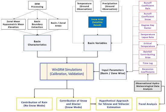
Figure 5.
Flowchart explaining methodology used in the study.
3.4.1. Structure of SRM
The SRM was developed by Martinec in 1975. The core advantage of the SRM is the requirement of minimal amounts of input data. This makes it most suitable for data sparse regions, e.g., HKH. The degree day method is used in most of the conceptual hydrological models because it requires the least amount of data [65]; it does not consider other energy components, especially the solar incoming radiation, besides wind parameters and latent heat of condensation. SRM parameters are very difficult to measure precisely in the field, therefore, they were mostly derived by analysis of recorded hydrological data, basin characteristics, and universal physical laws [66].
The structure of the SRM is based on the following equation:
where Q is the mean daily discharge [m3 s−1]; Cs and Cr are the runoff coefficients for snow for rain, respectively; a is the degree day factor (DDF) [cm °C−1 d−1] representing the depth of snow melt resulting from one degree day; T is the degree days [°C·d]; P is precipitation input to runoff [cm]; ∆T is the change in temperature, i.e., lapse rate for extrapolating the temperature recorded at the base station to the mean elevation of any zone [°C·d]; S is the fraction of snow in each elevation zone; A is the basin or zonal area [km2]; k represents the recession coefficient indicating the decline in discharge when there is no runoff from snow melt or rainfall; 10,000/86,400 is for converting cm·km2·d−1 to m3 s−1; and n represents the sequence of days of the discharge period.
The SRM consists of a graphical display of computed hydrographs against the measured runoff. The accuracy criteria of the SRM consists of the Nash–Sutcliffe Efficiency (NSE) measurements and the percent volume difference (%Dv).
The NSE value portrays the accuracy in daily computed flows against daily recorded flows and is as follows:
where is the recorded daily discharge, is the simulated daily discharge, and is the yearly averaged recorded discharge. The percent runoff volume, %Dv is computed as follows:
where is the measured yearly or seasonal runoff volume and is the computed yearly or seasonal runoff volume. Therefore, %Dv provides the error in annual computed volume against annual recorded volume.
3.4.2. Calibration and Validation of SRM
The first and most important step in the calibration of the SRM model was calculating the precise recession coefficient (k) value for the basin under study. By definition, “k” for each day is dependent on recession constants (x, y) and the previous day’s recorded streamflow as is evident from Equation (5).
If “k” values are appropriate, i.e., x, y constants are precisely derived, then the modelled streamflow will follow the pattern of recorded streamflow. The required constants were derived from historical recorded stream flows and hence, the SRM successfully achieved the pattern of recorded stream flows. The second step was the analysis of over and underestimation in the modelled stream flows against the recorded stream flows. It was achieved by calibrating the model input parameters (Table 1). The SRM is more sensitive to temperature lapse rate, followed by the degree day factor and runoff coefficients for rain and snow (Table 2). Therefore, initially, careful adjustments were carried out in those parameters to which the SRM is more sensitive. Graphical display and accuracy criteria (NSE and %Dv) were the indicators of a successful calibration (Section 4.2). The SRM was calibrated for 2008, 2009, and 2010.

Table 1.
Values of calibration parameters for SRM simulations.
Table 2.
Sensitivity analysis of SRM (Original Results: NSE = 0.966 and %Dv = −1.1165%).
The parameters of the SRM are shown in the flowchart presented in Figure 5. The time frame of 2000 to 2004 was selected for SRM validation (Table 3). TCRIT is the critical temperature deciding the type of precipitation either in form of rain or snow. For quantification of rainfall runoff and snow/glacier melt runoff, the model was executed in two separate modes, namely snow mode and no-snow mode. The no-snow mode provided the rainfall contribution to runoff for each year during the 1995–2010 period. The remaining river flow was taken as the contribution from snow and glacier melt.
Table 3.
Accuracy statistics for SRM simulations during the 1995–2010 period.
3.4.3. Sources of Uncertainty
The uncertainty starts with the input parameters of the SRM. The degree day factor is dependent on snow and ice densities as well as air temperatures [67] varying with time and space. Temperature lapse rate varies with altitude as well as with slope aspect and is even more complex based on time scales [68,69,70,71]. This means that the nature of lapse rate variation is temporally and spatially non-linear (heterogeneous), but is close to the global values (e.g., 0.63–0.65 °C per 100 m change in altitude) on average. As a result, we used long-term averaged values for temperature lapse rate. The situation is similar for other input parameters as well, such as runoff coefficients for rain and snow, due to their dependence on land cover and land use. Some uncertainties also exist in assigning monthly percentages to snow and glaciers. Uncertainties in spatial coverage and discontinuities in meteorological and hydrological data cause more trouble in runoff simulations and in conducting long-term studies.
4. Results
4.1. Trend Analysis of Meteorological and Hydrological Data
There are three high altitude meteorological stations in the HRB and one hydrological station measuring river discharge at Dainyour Bridge. The average annual temperatures of the stations at Naltar, Ziarat, and Khunjerab are 6.4 °C, 2.6 °C, and −5.5 °C, respectively. Statistical analysis showed that July was the hottest month each year. Recordings at these three stations indicated an annual average temperature lapse rate (TLR) of 0.62 °C per 100 m altitudinal change. The seasonal values equal the annual average temperature lapse rate value, but there are monthly variations. The model simulations were based on the observed monthly average TLR values. The TLR for July was 0.61, and 0.59 for August and September. Seasonal (winter and summer) and annual variations in temperature and precipitation are shown in Figure 6a–f. The average winter temperatures of the three stations showed an increasing trend of ~1.47 °C (during the 1995–2010 period), in contrast to a decreasing summer temperatures trend of ~0.33°C (Figure 6a–c). The decreasing summer trend was more gradual than the increasing trend in winter, resulting in a slightly increased annual trend (~0.6°C increase for the whole study period, i.e., during 1995–2010) in the observation. Figure 6a–c also shows the increase in winter temperatures at high altitudes compared to lower altitudes.
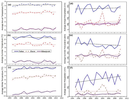
Figure 6.
The left side shows annual, summer, and winter temperatures from top to bottom (a–c), whereas the right side shows respective precipitation having the same pattern (d–f) during the 1995–2010 period from all three stations in the Hunza Basin. The blue solid line represents recordings at Naltar, the red dashed line at Ziarat, and the purple solid line at Khunjerab.
Precipitation varied laterally and with elevation during the sixteen-year period (1995–2010) with an average annual total of 182 mm, 228 mm, and 684 mm recorded at Khunjerab, Ziarat, and Naltar, respectively (Figure 6d). Note that the above mentioned total annual recorded precipitation with a decreasing trend with increasing in altitudes are not compatible with earlier studies [25,72,73], suggesting 5–10 times more precipitation at high altitudes than at the valley floor, thus leaving a question about the quality of the recorded data.
The winter precipitation showed an increasing trend at all three stations, while the summer precipitation showed a decreasing trend (Figure 6e–f). The total annual precipitation showed a general, non-monotonic increasing trend. The average annual precipitation averaged over all three stations over the sixteen years was 365 mm, which is very low compared to the estimates of 836 mm [74] and 1238 mm [75].
The seasonal precipitation pattern at Naltar and Ziarat was heterogeneous, with summer rainfall dominant in some years while winter rainfall was dominant in others. However, the summer precipitation recorded at the Khunjerab station was almost double the winter precipitation. The spatial variability of meteorological parameters in such complex terrain is always challenging [24,76] and cannot be fully covered by only three observation stations at the valley floor. Model simulations inherit these uncertainties in the observational data [75]. The increasing trend in recorded winter precipitation suggests more snow accumulation which is available for melting in summer, i.e., increases in summer river flows.
The decreasing summer temperatures (Figure 6) make it difficult to explain the reason behind increasing river flows. We, therefore, further investigated the available data by making groups of months (i.e., January, February, and March as JFM; April, May, and June as AMJ; July, August, and September as JAS; and October, November, and December as OND) (Figure 7). We found that the only difference between temperature and river flows is in the JAS group, as shown in the figure below. Furthermore, mass balance studies [32,38,55] showed slight negative mass balances, so the increased runoff is probably the result of excessive melting during the 1995–2010 period (Figure 7).
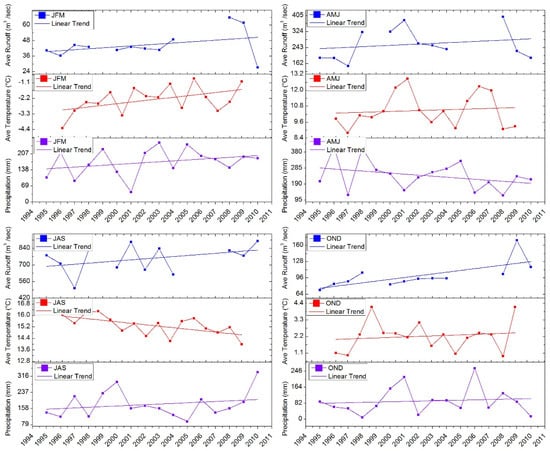
Figure 7.
Comparison among the recorded hydrological and meteorological data during the 1995–2010 period; grouped as JFM (January, February, March), AMJ (April, May, June), JAS (July, August, September), and OND (October, November, December).
River runoff was on the rise in all four groups which can be explained in groups JFM, AMJ, and OND (with a rise in temperature supported by an occasional rise in precipitation) but group JAS is exceptional, where temperatures showed a declining trend (Figure 7). However, precipitation was rising in the same group and supports the rise in runoff. Average temperatures were highest in this group among all four groups, and the decreasing trend was 0.08 °C per year during the 1995–2010 period. It is important to mention that warmer rain water over the glacier surface can cause accelerated melting called rain-induced melting [77,78,79]. We believe that this would have happened in study area as well. Moreover, the Hunza basin is a very complex basin and there are chances of missing heavy rain events and temperature recordings in sub-basins where there are no observation stations. At times, the quality of recorded data also limited the explanation of such situations.
Annual and seasonal flow were analyzed from the recorded hydrological data. Figure 8 shows the average monthly, seasonal, and annual river flows at the Dainyour Bridge on the Hunza River. The annual river flows showed a decreasing trend (Figure 8a), mostly dominated by summer flows (Figure 8b,c) during the 1966–2010 period. However, an increasing trend in annual flows was visible during 1995 and 2010 (Figure 8a). This increasing trend corroborates the increasing summer flows (Figure 7). On average, winter discharge contributed only 8% to the annual flows during the observation period, with only minor variations (Figure 8c). Further investigations revealed that the summer hydrographs were dominated by flows in July and August, with intermediate flows in June and September (Figure 8b).
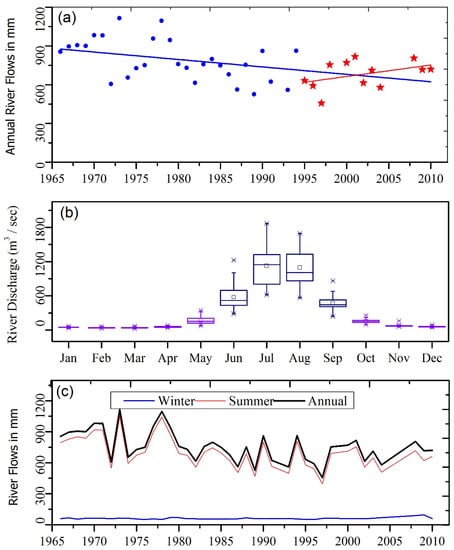
Figure 8.
(a) Annual river flows during 1966 and 2010 (stars indicate annual flows during 1995 and 2010 only) with linear trends. (b) Box plot of monthly flows during 1966 and 2010, dominated by flows in July and August followed by June and September. (c) Winter flows were very low, whereas summer and annual flows followed the same pattern which means annual flows are governed by summer flows.
4.2. SRM Simulations and Quantification of Runoff Components
The results of the SRM simulations for 1995–2010 are shown in Table 3 and Figure 9a–c. The Nash–Sutcliffe Efficiency (NSE) values show that the SRM performed effectively for most of the years with two exceptions, 1997 and 2000, where the model performed poorly (Figure 9a,b), as indicated by the values for NSE (−0.49, 0.564) and %Dv (−65.26%, −35.45%). The black line (Figure 9c) represents the observed river discharge data and the red line represents the SRM simulations. The model accurately simulated the low and high flows (Figure 9c), as confirmed by the accuracy assessment for the validation years shown in Figure 9b and for the calibration years in Figure 9a, with encouraging NSE values.
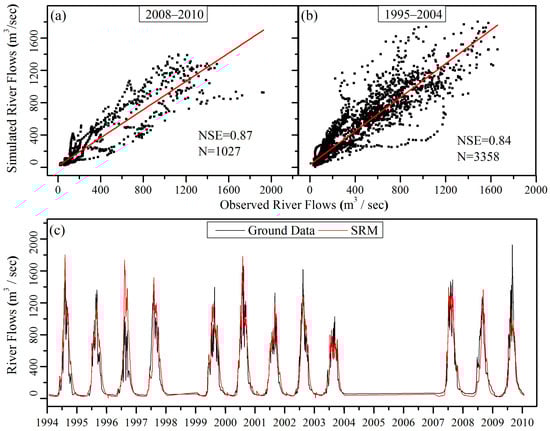
Figure 9.
(a) Simulated vs. recorded flows during calibration period (2008–2010). (b) Simulated flows versus observed flows during the validation period (1995–2004). (c) Comparison between observed and simulated flows in the Hunza River Basin during 1995 and 2010.
The poor performance in the years 1997 and 2000 were due to inefficient simulations of the flows in July, August, and September (summer months), and in May and July in the respective years. The SRM significantly overestimated the river flows during these specific periods. Further investigations of meteorological observations for the year 1997 revealed that the average monthly temperatures in July, August, and September were above the 16-year average temperatures. This suggest that more positive degree days were available for melting. Total monthly rainfall values were also above the long-term average for the year 1997. Total annual flow volume during this year were below average, so inconsistency in observation data is also possible. The meteorological data for the year 2000 showed that the rainfall remained above long-term monthly averages in the respective summer months. This appeared to be one of the reasons for an overestimation by the SRM for the year 2000. The simulations showed an overestimation of annual flow volume in 1995 and underestimation in 2010 (Figure 10c,d), as can be seen from the %Dv values (−25.63%, 23.37%), but were still good enough based on NSE values (0.85, 0.77). The SRM underestimated the annual flows in June, July, and August of 2010 and overestimated flows in July, September, and October in 1995. The rainfall recordings in June, July, and August of 2010 were well above the long-term averages, but the SRM showed underestimations. This means that the values of Cr for these respective months in 2010 were considered too low compared to the actual high values, hence, forcing the SRM to underestimate these values. The above average rainfall also suggests that there would be more melting if rainfall occurred on the surface of the snow and ice. The inconsistent simulations in 1995, 1997, 2000, and 2010 revealed that the SRM cannot simulate extreme scenarios where the conditions are not similar to the calibration year. This fact was also accepted by [80] that showed that models using calibrated parameters generally cope less well with extreme years and exceptional runoff situations. Above all, the inconsistent simulations may also occur due to limited amounts and quality of input data (temperature, precipitation, river flows), which mostly had to be interpolated to obtain the respective missing data.
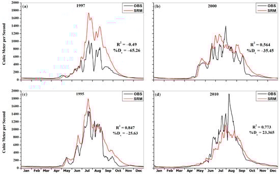
Figure 10.
(a–d): Inconsistent simulations by SRM for years 1995, 1997, 2000, and 2010.
The SRM performed well for the remaining years during the 1995–2010 period, with an average NSE value of 0.88 and %Dv value of −1.7. The detailed statistics are given in Table 3. To avoid any miscalculation due to over and underestimation, the rainfall runoff is subtracted from observational data for the snow–glacier components calculation.
5. Discussion
The estimated snow–glacier proportional contribution demonstrated that the glacier melt runoff component is explicitly dominant in the Hunza River Basin, e.g., 51.4% from glacier melt runoff on average during 1995 and 2010. The runoff derived from snow melt averaged 34.2% and runoff due to rainfall was 14.4% during the same period. [80] and [75] have used physically based distributed hydrological models for the quantification of runoff components in the HRB. Our results are comparable to those obtained by [81], who used a conceptual distributed hydrological model HBV (Hydrolo-giska Byråns Vatten-balansavdelning). This study estimated the average runoff contributions of 64%, 16.5%, and 19.4% from glacier melt, snow melt, and rain, respectively, to the Hunza River. However, [75] found contradictory percentages of snow and glacier melt runoff for the same basin, suggesting 50% of runoff was from baseflow and only 33% from glacier melt. Another study [51] obtained 38.73% as the total runoff contribution from snow and glacier melt whereas the base flow remained as the dominant contributor. The observational data in this study clearly depicted that the annual flows were governed by summer month flows (Figure 8c) where most of the seasonal snow has melted with some exceptions at higher altitudes; therefore, we adhere with our findings that glacier melt runoff should be dominant in summer and throughout the annual flows. Thus, a simple degree day model appeared to be successful in simulating comparable results with those by distributed hydrological models. Analysis of all of these investigations, including our own, indicated that individual contributions from snow and glacier melt may be different, but there is less disagreement on their combined effect, i.e., snow–glacier melt were collectively contributing 81–86% of the total runoff followed by 14–19% by rainfall (Table 4). Using a fully distributed hydrological model including all cryospheric processes, the authors of [33] measured the hydrological regimes of five major river basins in High Mountain Asia (HMA), including the UIB. Lutz [33] found that the UIB is dominated by glacier melt, contributing up to 40.6% of the total runoff. In an another study [38], it was reported that the Karakoram Mountains alone accommodate 70% of the glaciers in the UIB, indicating that the glacier melt runoff contribution would be greater than 40.6% as mentioned by Lutz [33]. It can therefore be assumed that the findings of our analysis i.e., the dominance of glacier melt runoff in HRB is valid. The results of this study corroborate with a few earlier studies validating the dominancy of melt runoff in flows of the Indus River and its tributaries. Thus, variations in river flows in the HKH region would be dominated by melt runoff i.e., fluctuations in the volume of glaciers.
Table 4.
Results comparison with similar studies in the Hunza basin.
Figure 11a,b shows the rain, snow, and glacier melt runoff percentages. The results showed that rainfall runoff was gradually decreasing, while melt runoff due to snow and glaciers was gradually increasing. As discussed in the results section, the temperature and precipitation data in JFM, AMJ, and OND months supported the rising melt runoff except for the July, August, and September (JAS) group throughout the study period. Only the temperature data showed a mismatch in Figure 7 whereas the precipitation data followed the rising pattern of melt runoff in all groups except for the April, May, and June group in Figure 7. The uncertainties in the model input parameters and hydrological and meteorological observations discussed in Section 3.4.3 may be the reason for mismatches in melt runoff trends and their causative factors. Similarly, remote sensing data also contain uncertainties in the estimation of the regional or basin-scale glacier mass balance, mainly due to coarse spatial resolution, seasonality of data acquisition, and density assumptions [27]. Besides the existing uncertainties, our results are corroborated by some recent studies. Brun et al. [32] calculated the total glacier mass change in the HMA from 2000 to 2016, and concluded that the Karakoram was a region of transition from positive to negative mass balance, implying a slight increase in glacier melting. Muhammad et al. [31] also reported slight mass losses of −0.02 ± 0.12 in the western Karakoram (Hunza) and a relatively more negative mass balance of −0.26 ± 0.21 m w.e. a−1 in the eastern (Shyok) Karakoram, which is in agreement with our results. Lutz et al. [33] concluded a slight decrease in the future snow melt runoff component in the UIB against our marginally rising pattern of the respective runoff component.
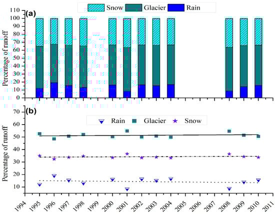
Figure 11.
Annual variations in runoff components between 1995 and 2010. (a): stacked percent snow, glacier melt runoff along with percent rainfall runoff of the respective years, (b): percent runoff components of the respective years.
The unavailability of consistent long-term data as well as desired spatial and temporal resolution of hydrological and meteorological observational data is still a challenge for an accurate explanation of the evidence of climate change in the basin. Nonetheless, the continuation of the ongoing increasing trend in melt runoff for yet another decade or more has the potential to predominantly affect the hydrology of the basin. Over time, it will affect the availability of fresh water at the right time for agriculture, besides other domestic and commercial uses. These challenges can be mitigated by developing water reservoirs to conserve and control the use of freshwater resources.
The comparison of our research with previous research work indicated that the quantification of melt runoff components and their long-term annual patterns have provided valuable information on the health of glaciers in the HRB and can be generalized globally in other glacierized regions.
6. Conclusions
Long-term river runoff trends (especially melt-runoff trends) can be a potential surrogate for mountain glacier changes. It is a widely accepted indicator of human-induced climate change worldwide. We used a satellite data-dependent degree day snowmelt runoff modeling approach to quantify the runoff components and assess their annual trends across the Hunza River Basin, i.e., one of the most densely glacierized sub-basins in the HKH region. For the period assessed (1950–2010), the temperature and precipitation data showed a rising trend in the winter, relatively higher than the summer reductions, resulting in slightly increased annual runoff trends. The decrease in JAS temperatures was inconsistent with the increase in river flows. The precipitation data showed a rising trend for the same period. The rising trends of river flows, especially the rise in melt runoff, were found to be supported by rising trends of precipitation, rain-induced melting, and possible missing information from recordings of heavy rain events.
The contributions of rainfall, snow, and glacier melt runoff components to river flows in the HRB were found to be 14.6%, 34.2%, and 51.2%, respectively. There are monotonic rising or declining patterns in runoff, but a gradual increase in snow and glacier melt was observed for the 1995–2010 period. This increased melting is considered an indicator of climate-induced change in the volume of glaciers in the study region.
There are indeed certain limitations of this study and the methods that were used in this study, e.g., discontinuity in the availability of observational hydrological and meteorological data, unavailability of daily cloud-free satellite images, unavailability of well-distributed recorded meteorological data both horizontally and vertically, and unavailability of actual parameter values in the study area. However, the consistency of the model results with mass balance studies of the same period and other studies confirms the usability of the SRM in other glaciated areas of the world. Such an approach can be especially useful for the areas where long-term mass balance studies are difficult to conduct. It can be concluded from this study that fluctuations in fresh water availability will occur due to climate-induced variations in melt runoff in the HRB. To cope with the freshwater fluctuations and possible shortages, effective management of the water supplies is advised, with a view to safeguarding the future water supply for the dependent population downstream.
Author Contributions
Conceptualization, M.H. and K.A.; methodology, M.H.; software, S.Q.; validation, K.A., M.H. and S.M.; formal analysis, M.H.; writing—original draft preparation, M.H.; writing—review and editing, T.B. and S.Q.; visualization, Z.H.; supervision, M.J.I. All authors have read and agreed to the published version of the manuscript.
Funding
This research received no external funding.
Institutional Review Board Statement
Not applicable.
Informed Consent Statement
Not applicable.
Data Availability Statement
The data presented in this study are available on request from the corresponding author.
Acknowledgments
We acknowledge the use of imagery from the USGS EarthExplorer and the Worldview Snapshots application https://wvs.earthdata.nasa.gov/ (accessed on 1 February 2022), part of the Earth Observing System Data and Information System (EOSDIS). We are also grateful to the Water and Power Development Authority (WAPDA) in Pakistan for the provision of hydrological and meteorological data. We further acknowledge that the article processing charge was funded by the Deutsche Forschungsge-meinschaft (DFG, German Research Foundation)—491192747 and the Open Access Publication Fund of Humboldt-Universität zu Berlin.
Conflicts of Interest
The authors declare no conflict of interest.
References
- Gourbesville, P. Challenges for integrated water resources management. Phys. Chem. Earth Parts ABC 2008, 33, 284–289. [Google Scholar] [CrossRef]
- Boretti, A.; Rosa, L. Reassessing the projections of the World Water Development Report. npj Clean Water 2019, 2, 15. [Google Scholar] [CrossRef]
- Mark, B.G.; Baraer, M.; Fernandez, A.; Immerzeel, W.; Moore, R.D.; Weingartner, R. Glaciers as water resources. In The High-Mountain Cryosphere, 1st ed.; Huggel, C., Carey, M., Clague, J., Kääb, A., Eds.; Cambridge University Press: Cambridge, UK, 2015; pp. 184–203. [Google Scholar] [CrossRef]
- Miller, J.D.; Immerzeel, W.W.; Rees, G. Climate Change Impacts on Glacier Hydrology and River Discharge in the Hindu Kush–Himalayas: A Synthesis of the Scientific Basis. Mt. Res. Dev. 2012, 32, 461–467. [Google Scholar] [CrossRef]
- Bolch, T.; Kulkarni, A.; Kääb, A.; Huggel, C.; Paul, F.; Cogley, J.G.; Frey, H.; Kargel, J.S.; Fujita, K.; Scheel, M.; et al. The State and Fate of Himalayan Glaciers. Science 2012, 336, 310–314. [Google Scholar] [CrossRef]
- IPCC. AR5 Climate Change 2013: The Physical Science Basis—IPCC. 2013. Available online: https://www.ipcc.ch/report/ar5/wg1/ (accessed on 14 August 2021).
- IPCC. Impacts, Adaptation, and Vulnerability, Part A: Global and Sectoral Aspects (GSA). 2014. Available online: https://www.ipcc.ch/report/ar5/syr/ (accessed on 14 August 2021).
- Bajracharya, S.R.; Maharjan, S.B.; Shrestha, F.; Guo, W.; Liu, S.; Immerzeel, W.; Shrestha, B. The glaciers of the Hindu Kush Himalayas: Current status and observed changes from the 1980s to 2010. Int. J. Water Resour. Dev. 2015, 31, 161–173. [Google Scholar] [CrossRef]
- World Glacier Monitoring Service (WGMS). Fluctuations of Glaciers Database; World Glacier Monitoring Service (WGMS): Zurich, Switzerland, 2017. [Google Scholar] [CrossRef]
- Kaser, G.; Fountain, A.; Jansson, P.; Heucke, E.; Knaus, M. A Manual for Monitoring the Mass Balance of Mountain Glaciers; Unesco: Paris, France, 2003; Volume 137. [Google Scholar]
- Huss, M.; Bookhagen, B.; Huggel, C.; Jacobsen, D.; Bradley, R.; Clague, J.; Vuille, M.; Buytaert, W.; Cayan, D.; Greenwood, G.; et al. Toward mountains without permanent snow and ice: Mountains without permanent snow and ice. Earths Future 2017, 5, 418–435. [Google Scholar] [CrossRef]
- Wester, P.; Mishra, A.; Mukherji, A.; Shrestha, A.B. (Eds.) The Hindu Kush Himalaya Assessment: Mountains, Climate Change, Sustainability and People; Springer International Publishing: Cham, Switzerland, 2019. [Google Scholar] [CrossRef]
- Scott, C.A.; Zhang, F.; Mukherji, A.; Immerzeel, W.; Mustafa, D.; Bharati, L. Water in the Hindu Kush Himalaya. In The Hindu Kush Himalaya Assessment; Wester, P., Mishra, A., Mukherji, A., Shrestha, A.B., Eds.; Springer International Publishing: Cham, Switzerland, 2019; pp. 257–299. [Google Scholar] [CrossRef]
- Dyurgerov, M. Mountain and subpolar glaciers show an increase in sensitivity to climate warming and intensification of the water cycle. J. Hydrol. 2003, 282, 164–176. [Google Scholar] [CrossRef]
- Huss, M.; Hock, R. A new model for global glacier change and sea-level rise. Front. Earth Sci. 2015, 3. [Google Scholar] [CrossRef]
- Marzeion, B.; Kaser, G.; Maussion, F.; Champollion, N. Limited influence of climate change mitigation on short-term glacier mass loss. Nat. Clim. Chang. 2018, 8, 305–308. [Google Scholar] [CrossRef]
- Shugar, D.H.; Jacquemart, M.; Shean, D.; Bhushan, S.; Upadhyay, K.; Sattar, A.; Schwanghart, W.; McBride, S.; de Vries, M.V.W.; Mergili, M.; et al. A massive rock and ice avalanche caused the 2021 disaster at Chamoli, Indian Himalaya. Science 2021, 373, 300–306. [Google Scholar] [CrossRef]
- Gautam, R.; Hsu, N.; Lau, W.-M.; Yasunari, T.J. Satellite observations of desert dust-induced Himalayan snow darkening: Dust-induced himalayan snow darkening. Geophys. Res. Lett. 2013, 40, 988–993. [Google Scholar] [CrossRef]
- Painter, T.H.; Deems, J.; Belnap, J.; Hamlet, A.; Landry, C.; Udall, B. Response of Colorado River runoff to dust radiative forcing in snow. Proc. Natl. Acad. Sci. USA 2010, 107, 17125–17130. [Google Scholar] [CrossRef] [PubMed]
- Muhuri, A.; Bhattacharya, A.; Natsuaki, R.; Hirose, A. Glacier surface velocity estimation using stokes vector correlation. In Proceedings of the 2015 IEEE 5th Asia-Pacific Conference on Synthetic Aperture Radar (APSAR), Singapore, 1–4 September 2015; pp. 606–609. [Google Scholar] [CrossRef]
- Huang, L.; Li, Z. Comparison of SAR and optical data in deriving glacier velocity with feature tracking. Int. J. Remote Sens. 2011, 32, 2681–2698. [Google Scholar] [CrossRef]
- Paul, F.; Bolch, T.; Briggs, K.; Kääb, A.; McMillan, M.; McNabb, R.; Nagler, T.; Nuth, C.; Rastner, P.; Strozzi, T.; et al. Error sources and guidelines for quality assessment of glacier area, elevation change, and velocity products derived from satellite data in the Glaciers_cci project. Remote. Sens. Environ. 2017, 203, 256–275. [Google Scholar] [CrossRef]
- Immerzeel, W.W.; van Beek, L.; Bierkens, M.F.P. Climate Change Will Affect the Asian Water Towers. Science 2010, 328, 1382–1385. [Google Scholar] [CrossRef] [PubMed]
- Tahir, A.A.; Chevallier, P.; Arnaud, Y.; Neppel, L.; Ahmad, B. Modeling snowmelt-runoff under climate scenarios in the Hunza River basin, Karakoram Range, Northern Pakistan. J. Hydrol. 2011, 409, 104–117. [Google Scholar] [CrossRef]
- Wake, C.P. Glaciochemical Investigations as a Tool for Determining the Spatial and Seasonal Variation of Snow Accumulation in the Central Karakoram, Northern Pakistan. Ann. Glaciol. 1989, 13, 279–284. [Google Scholar] [CrossRef]
- Hewitt, K.; Wake, C.; Young, G.; David, C. Hydrological Investigations at Biafo Glacier, Karakoram Range, Himalaya; an Important Source of Water for the Indus River. Ann. Glaciol. 1989, 13, 103–108. [Google Scholar] [CrossRef]
- Young, G.J.; Hewitt, K. Hydrology research in the upper Indus basin, Karakoram Himalaya, Pakistan. IAHS-AISH Publ. 1989, 190, 139–152. [Google Scholar]
- Archer, D.R.; Fowler, H.J. Spatial and temporal variations in precipitation in the Upper Indus Basin, global teleconnections and hydrological implications. Hydrol. Earth Syst. Sci. 2004, 8, 47–61. [Google Scholar] [CrossRef]
- Bookhagen, B.; Burbank, D.W. Toward a complete Himalayan hydrological budget: Spatiotemporal distribution of snowmelt and rainfall and their impact on river discharge. J. Geophys. Res. 2010, 115, F03019. [Google Scholar] [CrossRef]
- Archer, D. Contrasting hydrological regimes in the upper Indus Basin. J. Hydrol. 2003, 274, 198–210. [Google Scholar] [CrossRef]
- Muhammad, S.; Tian, L.; Khan, A. Early twenty-first century glacier mass losses in the Indus Basin constrained by density assumptions. J. Hydrol. 2019, 574, 467–475. [Google Scholar] [CrossRef]
- Brun, F.; Berthier, E.; Wagnon, P.; Kääb, A.; Treichler, D. A spatially resolved estimate of High Mountain Asia glacier mass balances from 2000 to 2016. Nat. Geosci. 2017, 10, 668–673. [Google Scholar] [CrossRef] [PubMed]
- Lutz, A.F.; Immerzeel, W.; Shrestha, A.; Bierkens, M.F.P. Consistent increase in High Asia’s runoff due to increasing glacier melt and precipitation. Nat. Clim. Chang. 2014, 4, 587–592. [Google Scholar] [CrossRef]
- Singh, P. Snow and Glacier Hydrology; Springer: Amsterdam, The Netherlands, 2001; Available online: https://www.springer.com/gp/book/9780792367673 (accessed on 14 August 2021).
- Akhtar, M.; Ahmad, N.; Booij, M.J. The impact of climate change on the water resources of Hindukush–Karakorum–Himalaya region under different glacier coverage scenarios. J. Hydrol. 2008, 355, 148–163. [Google Scholar] [CrossRef]
- Immerzeel, W.W.; Pellicciotti, F.; Bierkens, M.F.P. Rising river flows throughout the twenty-first century in two Himalayan glacierized watersheds. Nat. Geosci. 2013, 6, 742–745. [Google Scholar] [CrossRef]
- Adnan, M.; Nabi, G.; Kang, S.; Zhang, G.; Adnan, R.M.; Anjum, M.N.; Iqbal, M.; Ali, A.F. Snowmelt Runoff Modelling under Projected Climate Change Patterns in the Gilgit River Basin of Northern Pakistan. Pol. J. Environ. Stud. 2017, 26, 525–542. [Google Scholar] [CrossRef]
- Gao, H.; Zou, X.; Wu, J.; Zhang, Y.; Deng, X.; Hussain, S.; Wazir, M.A.; Zhu, G. Post-20th century near-steady state of Batura Glacier: Observational evidence of Karakoram Anomaly. Sci. Rep. 2020, 10, 987. [Google Scholar] [CrossRef]
- Bashir, F.; Zeng, X.; Gupta, H.; Hazenberg, P. A Hydrometeorological Perspective on the Karakoram Anomaly Using Unique Valley-Based Synoptic Weather Observations: Explaining the Karakoram Anomaly. Geophys. Res. Lett. 2017, 44, 10470–10478. [Google Scholar] [CrossRef]
- Hewitt, K. The Karakoram Anomaly? Glacier Expansion 332 and the ‘Elevation Effect,’ Karakoram Himalaya. Mt. Res. Dev. 2005, 25, 332–340. [Google Scholar] [CrossRef]
- Hewitt, K. Tributary glacier surges: An exceptional concentration at Panmah Glacier, Karakoram Himalaya. J. Glaciol. 2007, 53, 181–188. [Google Scholar] [CrossRef]
- Gardelle, J. Slight mass gain of Karakoram glaciers in the early twenty-first century. Nat. Geosci. 2012, 5, 322–325. [Google Scholar] [CrossRef]
- Asad, F.; Zhu, H.; Zhang, H.; Liang, E.; Muhammad, S.; Bin Farhan, S.; Hussain, I.; Wazir, M.A.; Ahmed, M.; Esper, J. Are Karakoram temperatures out of phase compared to hemispheric trends? Clim. Dyn. 2016, 48, 3381–3390. [Google Scholar] [CrossRef]
- Muhammad, S.; Tian, L. Changes in the ablation zones of glaciers in the western Himalaya and the Karakoram between 1972 and 2015. Remote Sens. Environ. 2016, 187, 505–512. [Google Scholar] [CrossRef]
- Qureshi, M.A.; Yi, C.; Xu, X.; Li, Y. Glacier status during the period 1973–2014 in the Hunza Basin, Western Karakoram. Quat. Int. 2017, 444, 125–136. [Google Scholar] [CrossRef]
- Gul, C.; Kang, S.; Ghauri, B.; Haq, M.; Muhammad, S.; Ali, S. Using Landsat images to monitor changes in the snow-covered area of selected glaciers in northern Pakistan. J. Mt. Sci. 2017, 14, 2013–2027. [Google Scholar] [CrossRef]
- Baig, S.U.; Khan, H.; Din, A. Spatio-temporal analysis of glacial ice area distribution of Hunza River Basin, Karakoram region of Pakistan. Hydrol. Process. 2018, 32, 1491–1501. [Google Scholar] [CrossRef]
- Shafique, M.; Faiz, B.; Bacha, A. Evaluating Glacier Dynamics Using Temporal Remote Sensing Images: A Case Study Of Hunza Valley, Northern Pakistan. Int. Arch. Photogramm. Remote Sens. Spat. Inf. Sci. 2019, XLII-2/W13, 1781–1785. [Google Scholar] [CrossRef]
- Muhammad, S.; Tian, L.; Nüsser, M. No significant mass loss in the glaciers of Astore Basin (North-Western Himalaya), between 1999 and 2016. J. Glaciol. 2019, 65, 270–278. [Google Scholar] [CrossRef]
- Khattak, M.; Babel, M.; Sharif, M. Hydro-meteorological trends in the upper Indus River basin in Pakistan. Clim. Res. 2011, 46, 103–119. [Google Scholar] [CrossRef]
- Ali, S.H.; Bano, I.; Kayastha, R.; Shrestha, A. Comparative Assessment of Runoff And Its Components in Two Catchments of upper Indus Basin by Using A Semi Distributed Glacio-Hydrological Model. Int. Arch. Photogramm. Remote Sens. Spat. Inf. Sci. 2017, XLII-2/W7, 1487–1494. [Google Scholar] [CrossRef]
- Bin Farhan, S.; Zhang, Y.; Aziz, A.; Gao, H.; Ma, Y.; Kazmi, J.; Shahzad, A.; Hussain, I.; Mansha, M.; Umar, M.; et al. Assessing the impacts of climate change on the high altitude snow- and glacier-fed hydrological regimes of Astore and Hunza, the sub-catchments of Upper Indus Basin. J. Water Clim. Chang. 2018, 11, 479–490. [Google Scholar] [CrossRef]
- Zhang, S.; Ye, B.; Liu, S.; Zhang, X.; Hagemann, S. A modified monthly degree-day model for evaluating glacier runoff changes in China. Part I: Model development: Evaluation of changes in glacier runoff in china. Hydrol. Process. 2011, 26, 1686–1696. [Google Scholar] [CrossRef]
- Zhou, Y.; Li, Z.; Li, J. Slight glacier mass loss in the Karakoram region during the 1970s to 2000 revealed by KH-9 images and SRTM DEM. J. Glaciol. 2017, 63, 331–342. [Google Scholar] [CrossRef]
- Bolch, T.; Pieczonka, T.; Mukherjee, K.; Shea, J. Brief communication: Glaciers in the Hunza catchment (Karakoram) have been nearly in balance since the 1970s. Cryosphere 2017, 11, 531–539. [Google Scholar] [CrossRef]
- Kääb, A.; Berthier, E.; Nuth, C.; Gardelle, J.; Arnaud, Y. Contrasting patterns of early twenty-first-century glacier mass change in the Himalayas. Nature 2012, 488, 495–498. [Google Scholar] [CrossRef]
- Hewitt, K. Glacier Change, Concentration, and Elevation Effects in the Karakoram Himalaya, Upper Indus Basin. Mt. Res. Dev. 2011, 31, 188–200. [Google Scholar] [CrossRef]
- Hewitt, K. Glaciers of the Karakoram Himalaya; Springer: Dordrecht, The Netherlands, 2014. [Google Scholar] [CrossRef]
- Racoviteanu, A.E.; Rittger, K.; Armstrong, R. An Automated Approach for Estimating Snowline Altitudes in the Karakoram and Eastern Himalaya From Remote Sensing. Front. Earth Sci. 2019, 7, 220. [Google Scholar] [CrossRef]
- Quincey, D.J.; Copland, L.; Mayer, C.; Bishop, M.; Luckman, A.; Belò, M. Ice velocity and climate variations for Baltoro Glacier, Pakistan. J. Glaciol. 2009, 55, 1061–1071. [Google Scholar] [CrossRef]
- Martinec, J.; Rango, A.; Roberts, R. WinSRM User’ s Manual for Windows; New Mexico State University: Las Cruces, NM, USA, 2008; p. 180. [Google Scholar]
- Muhuri, A.; Gascoin, S.; Menzel, L.; Kostadinov, T.S.; Harpold, A.A.; Sanmiguel-Vallelado, A.; Moreno, J.I.L. Performance Assessment of Optical Satellite-Based Operational Snow Cover Monitoring Algorithms in Forested Landscapes. IEEE J. Sel. Top. Appl. Earth Obs. Remote Sens. 2021, 14, 7159–7178. [Google Scholar] [CrossRef]
- Qiao, H.; Zhang, P.; Li, Z.; Liu, C. A New Geostationary Satellite-Based Snow Cover Recognition Method for FY-4A AGRI. IEEE J. Sel. Top. Appl. Earth Obs. Remote Sens. 2021, 14, 11372–11385. [Google Scholar] [CrossRef]
- Tsai, Y.-L.S.; Dietz, A.; Oppelt, N.; Kuenzer, C. Remote Sensing of Snow Cover Using Spaceborne SAR: A Review. Remote Sens. 2019, 11, 1456. [Google Scholar] [CrossRef]
- Hock, R. Temperature index melt modelling in mountain areas. J. Hydrol. 2003, 282, 104–115. [Google Scholar] [CrossRef]
- Martinec, J.; Rango, A.; Roberts, R. Snowmelt runoff model (SRM) user’s manual. In Geographica Bernensia P 35; Updated Edition for Windows; University of Bern: Bern, Switzerland, 2008. [Google Scholar]
- Asaoka, Y.; Kominami, Y. Incorporation of satellite-derived snow-cover area in spatial snowmelt modeling for a large area: Determination of a gridded degree-day factor. Ann. Glaciol. 2013, 54, 205–213. [Google Scholar] [CrossRef]
- McCutchan, M.H. Comparing Temperature and Humidity on a Mountain Slope and in the Free Air Nearby. Mon. Weather Rev. 1983, 111, 836–845. [Google Scholar] [CrossRef]
- Minder, J.R.; Mote, P.; Lundquist, J.D. Surface temperature lapse rates over complex terrain: Lessons from the Cascade Mountains. J. Geophys. Res. 2010, 115, D14122. [Google Scholar] [CrossRef]
- Gouvas, M.A.; Sakellariou, N.; Kambezidis, H.D. Estimation of the monthly and annual mean maximum and mean minimum air temperature values in Greece. Meteorol. Atmos. Phys. 2011, 110, 143–149. [Google Scholar] [CrossRef]
- Kattel, D.B.; Yao, T.; Yang, W.; Gao, Y.; Tian, L. Comparison of temperature lapse rates from the northern to the southern slopes of the Himalayas: Temperature lapse rates on the northern slopes of the Himalayas. Int. J. Climatol. 2015, 35, 4431–4443. [Google Scholar] [CrossRef]
- Mayer, C.; Lambrecht, A.; Belò, M.; Smiraglia, C.; Diolaiuti, G. Glaciological characteristics of the ablation zone of Baltoro glacier, Karakoram, Pakistan. Ann. Glaciol. 2006, 43, 123–131. [Google Scholar] [CrossRef]
- Immerzeel, W.W.; Pellicciotti, F.; Shrestha, A.B. Glaciers as a Proxy to Quantify the Spatial Distribution of Precipitation in the Hunza Basin. Mt. Res. Dev. 2012, 32, 30–38. [Google Scholar] [CrossRef]
- Immerzeel, W.W.; van Beek, L.; Konz, M.; Shrestha, A.; Bierkens, M.F.P. Hydrological response to climate change in a glacierized catchment in the Himalayas. Clim. Chang. 2012, 110, 721–736. [Google Scholar] [CrossRef]
- Shrestha, M.; Koike, T.; Hirabayashi, Y.; Xue, Y.; Wang, L.; Rasul, G.; Ahmad, B. Integrated simulation of snow and glacier melt in water and energy balance-based, distributed hydrological modeling framework at Hunza River Basin of Pakistan Karakoram region: Integrated snow and glaciermelt model. J. Geophys. Res. Atmospheres 2015, 120, 4889–4919. [Google Scholar] [CrossRef]
- Fowler, H.J.; Archer, D.R. Conflicting Signals of Climatic Change in the Upper Indus Basin. J. Clim. 2006, 19, 4276–4293. [Google Scholar] [CrossRef]
- Alexander, D.; Shulmeister, J.; Davies, T. High basal melting rates within high-precipitation temperate glaciers. J. Glaciol. 2011, 57, 789–795. [Google Scholar] [CrossRef]
- Doyle, S.H.; Hubbard, A.; Van De Wal, R.S.W.; Box, J.E.; van As, D.; Scharrer, K.; Meierbachtol, T.W.; Smeets, P.C.J.P.; Harper, J.T.; Johansson, E.; et al. Amplified melt and flow of the Greenland ice sheet driven by late-summer cyclonic rainfall. Nat. Geosci. 2015, 8, 647–653. [Google Scholar] [CrossRef]
- Fox, A. Rain Is Melting Greenland’s Ice, Even in Winter, Raising Fears about Sea Level Rise. Available online: https://www.science.org/content/article/rain-melting-greenland-s-ice-even-winter-raising-fears-about-sea-level-rise (accessed on 7 March 2019).
- Martinec, J.; Rango, A. Parameter values for snowmelt runoff modelling. J. Hydrol. 1986, 84, 197–219. [Google Scholar] [CrossRef]
- Ali, A.F.; Xiao, C.; Zhang, X.; Adnan, M.; Iqbal, M.; Khan, G. Projection of future streamflow of the Hunza River Basin, Karakoram Range (Pakistan) using HBV hydrological model. J. Mt. Sci. 2018, 15, 2218–2235. [Google Scholar] [CrossRef]
Disclaimer/Publisher’s Note: The statements, opinions and data contained in all publications are solely those of the individual author(s) and contributor(s) and not of MDPI and/or the editor(s). MDPI and/or the editor(s) disclaim responsibility for any injury to people or property resulting from any ideas, methods, instructions or products referred to in the content. |
© 2023 by the authors. Licensee MDPI, Basel, Switzerland. This article is an open access article distributed under the terms and conditions of the Creative Commons Attribution (CC BY) license (https://creativecommons.org/licenses/by/4.0/).