Quantifying Temperate Forest Diversity by Integrating GEDI LiDAR and Multi-Temporal Sentinel-2 Imagery

Abstract

Remotely sensed estimates of forest diversity have become increasingly important in assessing anthropogenic and natural disturbances and their effects on biodiversity under limited resources. Whereas field inventories and optical images are generally used to estimate forest diversity, studies that combine vertical structure information and multi-temporal phenological characteristics to accurately quantify diversity in large, heterogeneous forest areas are still lacking. In this study, combined with regression models, three different diversity indices, namely Simpson (λ), Shannon (H′), and Pielou (J′), were applied to characterize forest tree species diversity by using GEDI LiDAR data and Sentinel-2 imagery in temperate natural forest, northeast China. We used Mean Decrease Gini (MDG) and Boosted Regression Tree (BRT) to assess the importance of certain variables including monthly spectral bands, vegetation indices, foliage height diversity (FHD), and plant area index (PAI) of growing season and non-growing seasons (68 variables in total). We produced 12 forest diversity maps on three different diversity indices using four regression algorithms: Support Vector Machines (SVM), Random Forest (RF), K-Nearest Neighbors (KNN), and Lasso Regression (LR). Our study concluded that the most important variables are FHD, NDVI, NDWI, EVI, short-wave infrared (SWIR) and red-edge (RE) bands, especially in the growing season (May and June). In terms of algorithms, the estimation accuracies of the RF (averaged R² = 0.79) and SVM (averaged R² = 0.76) models outperformed the other models (R² of KNN and LR are 0.68 and 0.57, respectively). The study demonstrates the accuracy of GEDI LiDAR data and multi-temporal Sentinel-2 images in estimating forest diversity over large areas, advancing the capacity to monitor and manage forest ecosystems.

1. Introduction

Forests host unique tree species diversities, which support key ecosystem services such as nutrient cycles, head-water conservation, and biomass estimation [1]. Forest diversity is changing in response to climate change, soil erosion, species introductions and more [2]. In addition, forest productivity increases with tree species richness, and higher tree species diversity provides more food options for wildlife. Thus, developing effective technology is urgently needed for mapping forest diversity distribution over large areas to assess their current states and carrying capacity for animal populations [3].

Forest diversity is typically assessed by botanical surveys of the woods and metrics related to their species diversity (i.e., richness, Simpson, and Pielou diversity) [2,4]. Traditionally, forest diversity is calculated by counting the number and types of trees, which is an expensive, time-consuming process. Additionally, due to accuracy problems and difficulty in recognizing intertwined tree species, such a strategy is difficult to implement in large (e.g., hundreds of hectares) forest communities [5]. The challenges are more significant in natural forests with dense canopies. Remote sensing techniques have shown great potential for large-scale estimations of forest diversity and have been successfully used to estimate species diversity of subtropical and tropical forest ecosystems [6,7]. However, contemporary remote sensing-based approaches to estimate forest diversity vary with regard to the satellite data and machine learning models deployed. Plant richness of herbaceous ecosystems has been assessed using hyperspectral imagery by Oldeland et al. [3]. Nagendra et al. [7] used IKONOS and Landsat images to estimate forest species richness and diversity in central India. Stenzel et al. [8] used multi-seasonal, multi-spectral remote sensing data (RapidEye) to map ecological regions with high species richness. Almeida et al. [9] used hyperspectral images and airborne LiDAR data to assess the structure and diversity of restoration plantings. Clearly, rich spectral information plays an important role in species richness. However, these remote-sensing data are limited by area coverage, weather conditions, high costs, and acquisition time [10], making it challenging to develop detailed maps of forest diversity across large areas. Currently, commonly used methods for estimating forests diversity based on remote sensing data are extrapolated by using field data collected. Leutner et al. [11] examined the relationship between remotely sensed and field data, and mapped α- and β-diversity in the Yucatan Peninsula by using a regression kriging procedure. Hakkenberg et al. [12] predicted floristic diversity at different spatial scales using nonparametric models trained with spatially nested field plots and aerial LiDAR-hyperspectral data. Chrysafis et al. [13] developed a workflow to obtain tree diversity maps with machine learning algorithms using multispectral and multi-seasonal Sentinel-2 images and geodiversity data at the regional scale. The most important process in these methods is to extract features from remote sensing data, which are spectral indices or LiDAR-based metrics highly relevant to forest diversity, and then using these features as a set of mixed variables for regression analysis. Although these methods have achieved good prediction accuracy, it is unclear which types of algorithms are more effective in estimating forest diversity.

Sentinel-2 satellite data with 10 m spatial resolution has large spatial coverage, short acquisition time, and rich spectral bands that offer unprecedented opportunities to estimate tree species diversity [14]. The phenological differences of plant communities can be captured by their high temporal resolution and used as metrics to calculate plant diversity [15]. Detailed spectral information is related to plant biochemical composition, canopy structure, and leaf morphology characteristics, specifically for red-edge wavelengths [16]. Then, being available for free, they can be used to process large areas and complement field surveys at a reduced cost [17]. Sentinel-2 imagery has achieved good performance in mapping tree species classification [15], vegetation phenology monitoring [18], and forest aboveground biomass [19]. However, estimating tree species diversity is still lacking, especially in temperate mixed forests. Additionally, since April 2019, the NASA Global Ecosystem Dynamics Investigation (GEDI), a spaceborne LiDAR sensor in the International Space Station, has acquired footprint data with an average diameter of 25 m [20]. GEDI is a full waveform LiDAR that was created with the purpose of detecting vegetation structure [21] and provides an unprecedented sampling density, which could be an ideal structure parameter for estimating forest diversity [22]. Potapov et al. [23] combined GEDI LiDAR and Landsat to produce a global tree height map at a 30 m resolution. Liang et al. [24] quantified aboveground biomass dynamics of charcoal degradation in Mozambique using GEDI LiDAR and Landsat. These studies provide promising examples for the potential of GEDI-Sentinel data fusion to estimate forest diversity continuously across large extents.

In this study, GEDI LiDAR data and multi-temporal Sentinel-2 images were integrated to estimate forest diversity at the pixel level within natural forests in northeast China. Specifically, this study aims to: (1) quantify the relationships between forest diversity and variables from Sentinel-2 and GEDI LiDAR, (2) explore the effective algorithm for high precision mapping of forest diversity, and (3) map forest diversity by using GEDI LiDAR data and Sentinel-2 images for forest ecological assessment.

2. Materials

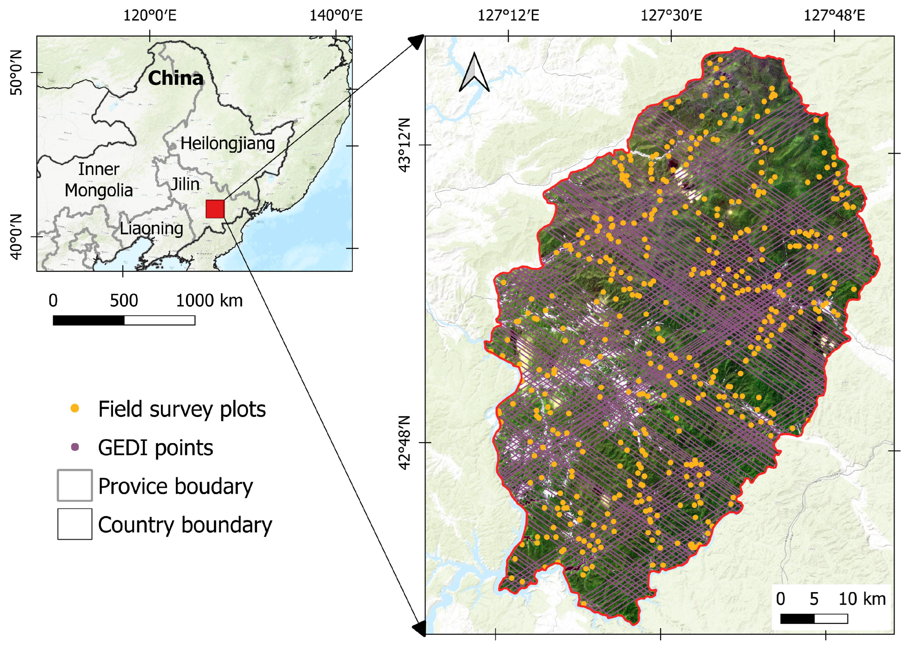
2.1. Study Area

The study area is located in the southeast region of Jilin Province, northeast China (Figure 1). It covers approximately 311,000 ha with an average elevation of 500 m. The average annual temperature ranges from nearly −3 to 7 °C, and the precipitation ranges from 500 mm to 1400 mm [25]. The forest types are mainly temporal mixed broadleaf-conifer woodlands, which are dominated by Juglans mandshurica, Pinus koraiensis, Betula costata, Larix gmelinii, Quercus mongolica, and Populus tremula.

2.2. Field Botanical Surveys

Compared with other forest parameters, forest diversity is related to spatial variability. Prior to field excursion, one would need to determine what size plots can achieve a stable range of spatial variability. In this study, we used the semi-variogram to determine the investigated plot size, which quantifies the spatial variability due to distance change [2]. Specifically, we calculated the square deviation between adjacent pixel values to test spatial variability with the Sentinel-based NDVI band. Semi-variance gradually increases with the distance between pixels until it starts to level off. Our findings indicated that lag distances of 50 m correspond to the scale for tree species variability in the study area (Appendix A, Figure A1). Thus, the plot size of 50 m × 50 m was identified as optimal in terms of capturing spatial variation in tree species diversity. From June to July 2019, field surveys were conducted. Based on spatial distribution randomness and road accessibility principles, a total of 452 plots were designed; The Global Positioning System was used to record each plot of position. In this study, based on the Chinese Forest Biodiversity Monitoring Network (CForBio) [26], all trees with a diameter at breast height (DBH) greater than 10 cm were identified, while trees with DBH less than 10 cm, shrubs and grasslands were not investigated considering the effect of dense canopy. In addition, the spatial distribution of different forest types was also obtained through the 9th National Forest Inventory of China (2018).

2.3. Data Source and Processing

2.3.1. Diversity Index Data

Based on sample data obtained from the field survey, tree species diversity for each plot was calculated using the three commonly used plant diversity indices, namely Shannon (H′), Simpson (λ) and Pielou (J′) (

Table 1. Three diversity indexes and corresponding equations were used in the study. Note: S is the total number of tree species in a plot; $P_i$ is the proportional abundance of species i relative to the total abundance of all species S in a plot; $In{P}_i$ is the natural logarithm of this proportion.

Diversity Index	Equation	Reference	Description
Shannon index (H′, based e)	$H^{\prime }=-{\displaystyle {\displaystyle \sum }_{i=1}^s}{P}_{i}In{P}_i$	[27]	Species richness and equitability in distribution in a plot
Simpson index (λ form)	$\lambda ={\displaystyle {\displaystyle \sum }_{i=1}^s}{P}_i^2$	[28]	The dominance of a species in a plot
Pielou evenness index (J′)	$J^{\prime }=\frac{-{{\displaystyle \sum }}_{i=1}^s{P}_{i}In{P}_i}{InS}$	[29]	How close in numbers each species in a plot

). Specifically, we first counted the species ($i$) and proportion ($P_i$) of trees in each plot, and then input the statistical parameters into the equations of diversity index to calculate diversity values of each plot (see Figure A2). Finally, the diversity values of each plot were used as dependent variables, and multi-variables from remote sensing data corresponding to the plot location were used as the prediction variables for the next step.

2.3.2. Sentinel-2 Images

Multi-temporal Sentinel-2 imagery was obtained from the Copernicus open access (COA) Hub [30]. We extracted 4 tiles of Sentinel-2 images which corresponded to different phenological phases and covered the study areas from May, June, September, and October in 2020. Using the Sen2Cor plug-in provided by the ESA [31], the Sentinel images were atmospherically corrected. In the sentinel application platform [32], bilinear interpolation method is used to resample all bands to 50 m, and then multiple vegetation indices were also calculated using Sentinel-2 bands (

Table 2. Vegetation indices extracted from Sentinel-2 satellite imagery.

Vegetation Indices	Expression	References
Normalized Difference Vegetation Index (NDVI)	$\frac{R_{nir}-R_{red}}{R_{nir}+R_{red}}$	[33]
Normalized Difference Water Index (NDWI)	$\frac{R_{nir}-R_{swir}}{R_{nir}+R_{swir}}$	[34]
Difference Vegetation Index (DVI)	$R_{nir}-R_{red}$	[35]
Enhanced Vegetation Index (EVI)	$2.5\left[\frac{R_{nir}-R_r}{L+R_{nir}+C_1{R}_r}\right]$	[36]
Soil Adjusted Vegetation Index (SAVI)	$\frac{R_{nir}-R_{red}}{L+R_{nir}+R_{red}}\ast \left(1+L\right)$	[37]

).

2.3.3. GEDI LiDAR Data

GEDI LiDAR L2B data were obtained from NASA Land Processes Distributed Active Archive Center (https://search.earthdata.nasa.gov/search, accessed on 21 October 2022) in 2019–2021, matching the region of study. The GEDI instrument acquired structural information, such as canopy height metrics, vertical profiles, and surface topography, by analyzing the amount of energy returned by various tree components at different heights above the ground [38]. In this study, the foliage height diversity (FHD) and plant area index (PAI) were extracted from 154,371 observations from GEDI L2B. The FHD index is a plant structural measure that describes the vertical heterogeneity of the foliage profile (

Table 3. Characteristics of data used in this study.

Data Type	Variables	Time	Description
Sentinel-2	B1	May. Jun. Sep. and Oct.	Coastal aerosol, 443 nm
	B2	May. Jun. Sep. and Oct.	Blue, 490 nm
	B3	May. Jun. Sep. and Oct.	Green, 560 nm
	B4	May. Jun. Sep. and Oct.	Red, 665 nm
	B5	May. Jun. Sep. and Oct.	Red edge, 705 nm
	B6	May. Jun. Sep. and Oct.	Red edge, 740 nm
	B7	May. Jun. Sep. and Oct.	Red edge, 783 nm
	B8	May. Jun. Sep. and Oct.	Near infrared, 842 nm
	B8A	May. Jun. Sep. and Oct.	Near infrared, 865 nm
	B11	May. Jun. Sep. and Oct.	Short-wave infrared, 1610 nm
	B12	May. Jun. Sep. and Oct.	Short-wave infrared, 2190 nm
Vegetation indices	NDVI	May. Jun. Sep. and Oct.	Normalized Difference Vegetation Index
	NDWI	May. Jun. Sep. and Oct.	Normalized Difference Water Index
	EVI	May. Jun. Sep. and Oct.	Enhanced Vegetation Index
	DVI	May. Jun. Sep. and Oct.	Difference Vegetation Index
	SAVI	May. Jun. Sep. and Oct.	Soil Adjusted Vegetation Index
GEDI LiDAR	FHD_NGS	Non-growing season	Foliage height diversity in non-growing season
	FHD_GS	Growing season	Foliage height diversity in growing season
	PAI_NGS	Non-growing season	Plant area index in non-growing season
	PAI_GS	Growing season	Plant area index in growing season

) [39]. The PAI, which comprises various plant components (stem, branches, and leaves), is the one-sided area of plant material surface per unit ground surface area [39]. Considering the changes in forest structure caused by phenological differences, we differentiated the two metrics as growing season and non-growing season. Considering the signal-to-noise ratio of the waveform, the sensitivity of a GEDI footprint shows the dense canopy cover that can be penetrated. Thus, we excluded footprints with sensitivity less than 0.9. After filtering out these invalid observations, 62,593 pairs of FHD and PAI were used for further processing.

To obtain spatially continuous FHD and PAI, we used inverse distance weighting (IDW) interpolation to achieve wall-to-wall diversity mapping. The IDW, as a global interpolation, is usually used for sample datasets that are uniformly distributed and dense enough to reflect local differences [40]. Measured values closest to the predicted location have a greater effect on the predicted value than those farther away, resulting in sensitivity of IDW interpolation to outliers and sampling configurations (i.e., clustering and isolation points) [41]. Thus, we randomly select dense GEDI points until these points are uniformly distributed throughout the study area. Then, we selected 80% of GEDI points for interpolation and parameter optimization and applied the remaining sample data (20%) for validation until the correlation coefficient was higher than 0.8.

3. Methods

3.1. Variable Importance Assessment

Selecting the most important variables from high-dimensional datasets is beneficial in improving efficiency and reducing model overfitting. In this study, Boosted Regression Tree (BRT) and Mean Decrease Gini (MDG) algorithms were used to evaluate the importance of independent variables. MDG indicates the contribution of each variable to the homogeneity of the nodes and leaves in the resulting random forest, while BRT evaluates variable performance by iteratively fitting and combining multiple regression tree models [42]. Both algorithms are capable of ingesting multiple classes of predicted variables to model complex interactions without making assumptions about variable interactions and have been widely used in ecological and remote sensing research [43].

3.2. Algorithms for Forest Diversity Mapping

In this study, four machine-learning algorithms with various setups were employed: Lasso Regression (LR), Random Forest (RF), K-Nearest Neighbors (KNN), and Support Vector Machine (SVM). Non-parametric, non-linear algorithms including KNN, RF, and SVM have been applied successfully in a variety of remote sensing applications [44]. KNN and SVM represent distance-based and kernel-based models, respectively, while RF represents tree-based models. Specifically, KNN finds similarities between the new data and available results and puts the new results into the category most similar to those available. SVM can hold regression problems with multidimensional data by separating positive and negative samples to identify the optimum decision hyperplane [45]. RF is a classifier containing a large number of decision tree classifiers [46], and each tree is trained with randomly selected training samples to solve a single problem [47]. All algorithms were implemented using the Scikit-learn python library, and the hyperparameters of LR, K-NN, SVM, and RF methods were fitted through cross-validation (

Table 4. Description of the regression models used in this study, including the parameters considered and the criteria used to rank the feature importance.

Model	Abbr.	Parameters	Feature Rank Criteria
Lasso regression	LR	—	Absolute value of coefficients
K-Nearest Neighbors	KNN	K values = 3, 5, 7, 9, 11	Minimum error rate
Support Vector Machine	SVM	cost = 0.1, 0.5, 1, 2, 4, 10	Squared weights
		kernel = linear, radial, sigmoid, rbf.
Random Forest	RF	ntree = 200, 500, 800, 1000	Increase in mean squared error by permuting a variable
		mtry = 2, 5, 10, 20, or k/3

) [48].

3.3. Accuracy Assessment

The coefficient of determination (${\mathrm{R}}^2$), root-mean-square error (RMSE) and mean absolute error (MAE) were applied to assess the accuracy of tree species diversity estimation. The following equations were used to calculated ${\mathrm{R}}^2$, RMSE, and MAE:

$${\mathrm{R}}^2=1-\frac{{{\displaystyle \sum }}_{\mathrm{i}=1}^{\mathrm{n}}{\left({\mathrm{y}}_{\mathrm{i}}-{\mathrm{x}}_{\mathrm{i}}\right)}^2}{{{\displaystyle \sum }}_{\mathrm{i}=1}^{\mathrm{n}}{\left({\mathrm{y}}_{\mathrm{i}}- \overline{\mathrm{y}}\right)}^2}$$

(1)

$$\mathrm{RMSE}=\sqrt{\frac{{{\displaystyle \sum }}_{\mathrm{i}=1}^{\mathrm{n}}{\left({\mathrm{x}}_{\mathrm{i}}-{\mathrm{y}}_{\mathrm{i}}\right)}^2}{\mathrm{n}}}$$

(2)

$$\mathrm{MAE}=\frac{{{\displaystyle \sum }}_{\mathrm{i}=1}^{\mathrm{n}}\left|{\mathrm{x}}_{\mathrm{i}}-{\mathrm{y}}_{\mathrm{i}}\right|}{\mathrm{n}}$$

(3)

where ${\mathrm{x}}_{\mathrm{i}}$ and ${\mathrm{y}}_{\mathrm{i}}$ are the estimated and measured values, respectively. $\overline{\mathrm{y}}$ is the average measured values, and n is the sample number.

All samples were randomly assigned to one of the two sets of training and validation, following the ratio of 70%:30%. Then, k-fold cross validation was also employed. The generalization error of a given method is directly estimated by cross-validation: The data is divided into K folds of almost equal size, and K folds are used to fit the model. Additionally, the estimated generalization error is the average error over the K folds.

4. Results

4.1. Optimal Features from SENTINEL-2 Images and GEDI LiDAR Data

MDG and BRT algorithms were applied to analyze the 68 features obtained by Sentinel-2 images and GEDI LiDAR data to find the optimal features for diversity mapping. Cross-validation is further used to score several feature subsets and choose the best scoring feature collection. Figure 2 shows the ranking results of key features for three diversity indices, other detailed results are displayed in Appendix A,

Table A1. Detailed results of variables importance.

	Simpson			Shannon			Pielou
Rank	Variables	BRT (%)	MDG (%)	Variables	BRT (%)	MDG (%)	Variables	BRT (%)	MDG (%)
1	FHD_GS	16.49	14.07	FHD_GS	15.59	12.14	NDVI_Jun	11.43	11.34
2	NDVI_Jun	12.16	12.37	NDVI_Jun	12.78	8.52	FHD_GS	9.33	7.48
3	NDWI_May	7.74	8.91	NDWI_May	10.48	9.38	NDWI_Jun	8.51	3.97
4	PAI_GS	7.55	6.33	B12_May	7.59	7.09	NDWI_May	5.38	5.07
5	NDWI_Jun	5.25	5.66	NDVI_Oct	6.40	6.84	PAI_GS	4.72	3.77
6	B12_May	4.58	5.55	PAI_GS	2.10	4.73	B12_May	3.97	2.94
7	EVI_May	5.18	3.84	B11_Oct	4.11	3.40	EVI_May	2.95	2.38
8	NDVI_May	3.75	3.18	EVI_May	3.52	2.70	B11_Oct	2.83	2.42
9	B12_Oct	3.21	2.76	B7_Jun	2.77	2.37	B7_Jun	2.77	2.40
10	B7_Jun	2.91	2.47	B11_Jun	2.36	2.25	B11_Jun	2.70	2.06
11	B11_Oct	2.58	2.25	B12_Oct	2.07	2.23	B12_Oct	1.66	2.02
12	B8A_Jun	1.97	2.18	NDVI_May	1.83	1.94	NDVI_May	1.59	1.68
13	B6_Jun	1.71	1.80	B8A_Jun	1.43	1.85	B5_May	1.59	1.45
14	B2_Jun	1.46	1.56	B8A_May	1.32	1.46	B8A_May	1.50	1.41
15	FHD_NGS	1.27	1.10	FHD_NGS	1.20	1.46	B5_Jun	1.49	1.40
16	B11_May	1.15	1.02	EVI_Oct	1.26	1.34	B8A_Jun	1.44	1.29
17	B1_Jun	0.92	0.99	B1_May	1.14	1.29	B5_Sep	1.29	1.18
18	NDWI_Sep	0.85	0.87	B8_Jun	1.08	1.19	NDVI_Oct	1.16	1.17
19	B4_May	0.83	0.85	DVI_Sep	1.02	1.05	B3_Sep	1.15	1.17
20	B3_May	0.78	0.84	B5_Oct	1.02	1.03	B3_Oct	1.11	1.16
21	B1_May	0.76	0.79	EVI_Jun	0.98	1.00	B4_Oct	1.09	1.13
22	B7_Sep	0.75	0.78	DVI_Oct	0.96	0.82	B7_Sep	1.07	1.12
23	B1_Oct	0.74	0.77	B3_May	0.89	0.80	B6_Sep	1.05	1.11
24	EVI_Oct	0.74	0.71	B4_May	0.89	0.78	B1_May	1.05	1.11
25	B6_Sep	0.71	0.69	B5_Jun	0.84	0.75	B1_Oct	1.04	1.09
26	B5_Jun	0.70	0.67	B1_Oct	0.78	0.75	B4_Sep	0.99	1.06
27	DVI_Sep	0.69	0.60	B12_Jun	0.75	0.72	B2_Oct	0.97	1.05
28	B12_Jun	0.68	0.60	B4_Sep	0.66	0.72	B1_Jun	0.97	1.05
29	B5_Sep	0.65	0.59	B2_Jun	0.65	0.69	DVI_Sep	0.97	1.04
30	B11_Jun	0.65	0.58	B3_Sep	0.62	0.68	B2_Sep	0.96	1.03
31	DVI_Oct	0.60	0.58	B5_May	0.61	0.68	PAI_NGS	0.95	1.03
32	B8_Jun	0.56	0.55	B1_Jun	0.61	0.65	DVI_Jun	0.93	1.00
33	NDVI_Oct	0.56	0.55	B2_Sep	0.57	0.64	DVI_Oct	0.93	0.99
34	PAI_NGS	0.55	0.49	B2_Oct	0.55	0.63	B6_May	0.85	0.98
35	DVI_Jun	0.54	0.49	B7_Sep	0.50	0.61	B6_Jun	0.84	0.98
36	B2_Oct	0.51	0.49	NDWI_Sep	0.48	0.61	B4_May	0.82	0.96
37	B8_Oct	0.48	0.48	B8_May	0.45	0.61	EVI_Oct	0.82	0.94
38	B9_Oct	0.48	0.47	NDWI_Oct	0.44	0.56	B9_Oct	0.80	0.92
39	B3_Jun	0.47	0.44	B6_May	0.44	0.54	B3_Jun	0.77	0.91
40	B3_Sep	0.47	0.43	B8A_Sep	0.43	0.52	B1_Sep	0.73	0.88
41	B3_Oct	0.46	0.42	NDWI_Jun	0.41	0.51	B5_Oct	0.73	0.88
42	B5_Oct	0.46	0.41	B11_May	0.40	0.51	B8_Jun	0.72	0.88
43	B2_Sep	0.31	0.40	B1_Sep	0.39	0.50	B2_May	0.71	0.86
44	B1_Sep	0.31	0.40	B6_Oct	0.37	0.49	EVI_Jun	0.71	0.85
45	B8A_Sep	0.30	0.39	B12_Sep	0.37	0.48	B12_Jun	0.70	0.85
46	B4_Oct	0.30	0.39	B6_Jun	0.36	0.48	NDVI_Sep	0.70	0.85
47	B2_May	0.28	0.39	DVI_Jun	0.36	0.47	B8A_Sep	0.70	0.84
48	B8_May	0.28	0.39	B8_Oct	0.31	0.47	B11_May	0.68	0.83
49	EVI_Jun	0.27	0.38	B5_Sep	0.30	0.46	B3_May	0.65	0.83
50	B4_Sep	0.26	0.38	NDVI_Sep	0.30	0.45	SAVI_May	0.56	0.83
51	NDWI_Oct	0.24	0.37	B6_Sep	0.30	0.45	SAVI_Sep	0.55	0.81
52	B5_May	0.24	0.37	B2_May	0.29	0.45	B8_Oct	0.53	0.81
53	B7_Oct	0.21	0.37	B11_Sep	0.28	0.43	FHD_NGS	0.52	0.81
54	B8A_May	0.20	0.37	PAI_NGS	0.26	0.42	B6_Oct	0.52	0.81
55	B6_Oct	0.19	0.37	B7_May	0.23	0.42	B11_Sep	0.50	0.79
56	B11_Sep	0.19	0.36	B9_Oct	0.22	0.42	B8_Sep	0.48	0.79
57	B8_Sep	0.18	0.36	B3_Oct	0.21	0.41	B4_Jun	0.48	0.77
58	B12_Sep	0.18	0.35	B4_Jun	0.19	0.41	B7_May	0.48	0.77
59	NDVI_Sep	0.16	0.33	SAVI_Sep	0.15	0.41	B2_Jun	0.47	0.77
60	B4_Jun	0.15	0.33	B4_Oct	0.07	0.40	B8_May	0.45	0.75
61	B6_May	0.13	0.32	DVI_May	0.02	0.40	DVI_May	0.33	0.73
62	DVI_May	0.03	0.31	B7_Oct	0.02	0.39	B12_Sep	0.30	0.72
63	SAVI_May	0.01	0.29	B8_Sep	0.02	0.39	B7_Oct	0.22	0.72
64	B7_May	0.00	0.27	SAVI_May	0.01	0.38	NDWI_Oct	0.17	0.67
65	SAVI_Sep	0.00	0.27	B3_Jun	0.00	0.37	SAVI_Jun	0.00	0.66
66	SAVI_Jun	0.00	0.25	SAVI_Jun	0.00	0.34	EVI_Sep	0.00	0.65
67	EVI_Sep	0.00	0.24	EVI_Sep	0.00	0.33	SAVI_Oct	0.00	0.65
68	SAVI_Oct	0.00	0.20	SAVI_Oct	0.00	0.32	NDWI_Sep	0.00	0.65

. Using the FHD and PAI of GEDI LiDAR in growing season, the vegetation indices of NDVI, NDWI, and EVI, and the spectral bands of B7, B8A, B11, and B12 were identified. Compared with individual spectral bands, GEDI feature and vegetation indices have a stronger explanation on the variations of forest diversity.

After feature selection, we applied mixed features from GEDI LiDAR data and Sentinel-2 images to estimate forest diversity. For comparison, we selected RF model and applied only GEDI LiDAR data or Sentinel-2 images for forest diversity estimation. Our results show that the Sentinel-2 data alone (averaged R² = 0.62) gives better prediction accuracies than the GEDI LiDAR data alone (averaged R² = 0.51), but both are lower than that of combined data sources (

Table 5. Estimated accuracy for different data combinations in three diversity indices.

Combined Variables	H′ Index		λ Index		J′ Index
	R2	RMSE	R2	RMSE	R2	RMSE
GEDI	0.51	0.78	0.54	0.26	0.48	0.35
Sentinel-2 &VIs	0.66	0.56	0.57	0.15	0.63	0.18
GEDI & Sentinel-2 &VIs	0.72	0.46	0.78	0.14	0.86	0.11

). Specifically, the Sentinel-2&VIs has a good performance on the prediction of H′ and J′ indices, with R² values of 0.66 and 0.63, RMSE of 0.56 and 0.18, although the result of λ index is slightly lower than other indices (R² = 0.57, RMSE = 0.15). The GEDI data alone is observed to have a relatively high prediction on H′ and λ indices (R² = 0.51; R² = 0.54 respectively), but a lower prediction on J′ index (R² = 0.48).

4.2. Diversity Indices Modelling Using Machine Learning Algorithms

Based on selected optimal predictor variables from Sentinel-2 and GEDI data, three diversity indices were characterized using LR, K-NN, RF, and SVM models. Our results showed that the R² values of all models are above 0.45 in all the diversity indices (Figure 3). Specifically, the RF model exhibited the best performance with R² = 0.86 (RMSE = 0.11) for the J′ index, 0.78 (RMSE = 0.15) for the λ index, and 0.73 (RMSE = 0.47) for H′ index (Figure 3a,e,i). The SVM also had positive results on the H′ and λ indices, with R² values of 0.80 and 0.72, RMSE of 0.37 and 0.16, although the result of the J′ index was lower than the other models (R² = 0.57, RMSE = 0.21) (Figure 3b,f,j). The KNN and LR models showed relatively low results on the λ index (R² = 0.46 and 0.57, respectively) (Figure 3c,d) but higher results on the J′ index (R² = 0.81 and 0.71, respectively) (Figure 3k,l). Overall, the main trend was that lower values of the three indices were a bit overestimated (above the 1:1 line) while high values were underestimated (below the 1:1 line).

4.3. Spatial Variability of the Predicted Diversity Indices

Based on the four regression models, we plotted the spatial variation of diversity indices and predicted variables within forests. The spatial distribution of the three diversity indices for the RF result is displayed in Figure 4, while the other results are displayed in Appendix A, Figure A3. Visually, the predicted maps show strong spatial agreements between the H′ and J′ indices, which are negatively related to the λ index in most parts of a forest. The H′ and λ indices account for species richness (i.e., number of different species) and abundance (i.e., number of individual trees per species), while J′ index accounts for species evenness (i.e., the numerical dominance of a few abundant tree species). Generally speaking, forest diversity was higher in the north than in the south, especially in the northeast. It is worth noting that the forest diversity of the sparse woods in the southwest area is significantly lower than that of other regions.

There are notable differences in tree species diversity according to the various forest types obtained by the 9th National Forest Inventory of China (2018). The diversity of the secondary forest regions (the right part of Figure 5a) could be easily distinguished from the natural forests based on predicted variables (Figure 5b–d). However, the performance varies amongst the three indices. Compared with other regions, the diversity of areas along rivers and roads did not significantly differ, but the J′ index along rivers expressed relatively low values (Figure 5f–h,j–l). Although the best prediction results were obtained by testing four regression models, we found that a single indicator does not adequately characterize diversity. For example, on the right side of the road in Figure 5f–h, there are significant differences in the three diversity indices, which forced us to obtain a more comprehensive assessment of diversity.

5. Discussion

5.1. Prospects of GEDI LiDAR and Sentinel-2 Data on Forest Diversity

In this study, we succeeded in estimating forest diversity in a mixed broadleaf-conifer forest, using multi-temporal Sentinel-2 and GEDI LiDAR data. This suggests promising potential for LiDAR data and optical images, combined with machine-learning approach, to estimate forest species diversity over large areas. Such a method would greatly improve conservation and management of forest resources. GEDI LiDAR data uses the reflected laser energy within ~25 m footprints to determine the height, canopy cover, and vertical distribution of plant material. This study is the first to apply the GEDI-derived FHD metrics to forest diversity estimation, our results demonstrate the importance of FHD metrics in future diversity studies. In forest ecology, a high FHD value typically indicates a more complex forest structure (e.g., caused by multiple canopy layers). Structure differences across tree species provide a different directional gap probability, which underlies the LiDAR-based estimations of forest diversity and were confirmed by the direct correlations between tree species diversity by indices (H′, λ and J′) and GEDI-derived FHD and PAI indices (Figure 6). Therefore, GEDI LiDAR data will become one of the most important parameters in forest diversity estimation. Nonetheless, we argue that it is difficult to achieve good performance using only GEDI data. Our study demonstrated that combined remote sensing data sources were better than GEDI LiDAR data or Sentinel-2 images alone in explaining tree species diversity. The higher explanatory power of the combined data sources was attributed to the full utilization of vegetation properties (vegetation structure information, biochemical properties, and phenological variability).

Unique spectral responses are caused by differences in the physical and chemical characteristics of various tree species, which is the main driver of forest diversity estimation. Compared to band features, vegetation indices (NDVI, NDWI, EVI, and SAVI) were more significantly correlated with forest diversity (H′, λ and J′). These results coincide with those reported by Madonsela et al. [2]. Vegetation indices enhance the spectral information from vegetation while limiting the spectral reflectance from non-vegetative characteristics [49]. This is also proven in Figure 7: The correlation coefficient between predicted H′ index and vegetation indices in the fall season is significantly higher than that of the band features. Variability in vegetation indices is caused by a variety of vegetation properties, such as photosynthetic pigments, biomass, and structural carbohydrates [50]. Thus, it is unsurprising that vegetation indices have a significant relationship with forest diversity indices (H′, λ and J′). Additionally, the value of Red-Edge, NIR, and SWIR bands for estimating plant diversity has been demonstrated in previous studies by Sothe et al. [51] and Grabska et al. [52]. This study also confirmed the importance of these bands using the BRT and MDG algorithm (see Figure 2). This success is attributed to the rich spectral band setting in Sentinel-2, for example, NIR and SWIR bands are sensitive to water content, lignin, starch, and nitrogen [53]. In addition, we noticed that the correlation coefficients of growing season and non-growing seasons showed a great gap, especially for spectral features. Seasonal variations in canopy structure and biochemical characteristics among several tree species were captured by the spectral values and vegetation indices. These differences provide important references for estimating forest diversity in various forest environments.

5.2. Machine Learning Algorithms for Forest Diversity Mapping

Four different types of machine-learning algorithms were used to estimate forest diversity indices, with three of the diversity indices used having their own variable selection. Our results showed that RF and SVM models provided the highest estimation accuracy in terms of the highest R², the lower RMSE, and MAE. This was confirmed by the KNN and LR models. The RF classifier, as an ensemble approach, consisted of a number of tree classifiers, which reduces overfitting impacts and has been the most often used in remote sensing tasks [54]. Similarly, SVMs are a high-performance method designed to solve nonlinear problems using various kernel functions, such as the radial basis function [55]. The solid performance of RF and SVM models were confirmed in other studies [56,57]. For λ and J′ indices, RF has the best prediction result, while in the H′ index, the SVM model is best. The kernel-based algorithm (e.g., SVM) is prone to overfitting when presented with an extreme value that cannot be identified in the sample [57]. In contrast, tree-based algorithms (e.g., RF) seem to be more resistant to overfitting, though they do not fit as well as kernel-based algorithms [58].

5.3. Prediction Performance and Uncertainty for Forest Diversity

Among the three diversity indices, J′ index has the highest correlation coefficient (R² = 0.86), followed by H′ index (R² = 0.80) and λ index (R² = 0.78). The three diversity indices, being different representations of plant diversity, varied in spatial distribution (Figure 5). λ index, which accounts for the proportion of species in a sample, is considered to be a dominance indicator [59]. H′ index reflects both species richness and equitable distribution of those species within a sample [3]. Moreover, Oldeland et al. [3] emphasized that the H′ index better mirrors what one could call “vegetation structure”, which is a subset of habitat heterogeneity and thus better reflects spectral variability. The spatial difference between the two indices has been well demonstrated in natural forests and secondary forests (Figure 5b,d). The J′ index is an indication of dominance and distribution of individuals across the community within a sample. Relatively few studies have reported this index in remote sensing studies, but it is still of great significance, especially considering the landscape scale [60].

While we derived the forest diversity map with high accuracy, several issues that may limit further estimations still exist. The first is the uncertainty of on-site measurements. In this study, we used semi-variance to determine a spatial scale for forest diversity investigation. Although fixed spatial scales are highly efficient in field surveys, they do not adequately represent the diversity values of the survey region [61]. Secondly, the presence of rare tree species in the understory and trees with DBH less than 10 cm may bring uncertainty on the estimation of forest diversity. Our study area is primarily composed of protected pristine natural forests [27], and the DBH of most trees exceeds 10 cm, which is also confirmed in field surveys. Thus, these trees have no impact on the experimental design and analysis, especially under dense canopy [49]. Finally, errors already exist in the process of forest diversity prediction. For example, the background, including the shading caused by tree canopy, topography, and/or soil color, could cause biased reflectance captured by Sentinel-2 [62].

6. Conclusions

In this study, we applied machine-learning-based regression models to map the spatial patterns of forest diversity in a temperate mixed forest in northeast China. We did this by coupling the newly available diversity product from GEDI LiDAR and multi-temporal Sentinel-2 imagery. Our results showed that a variety of diversity indices can be predicted accurately through combining forest vertical structure information, plant biochemistry, and phenological variability. More accurately, utilizing the FHD index from GEDI, vegetation indices (NDVI, NDWI and EVI), and shortwave infrared band from Sentinel-2 imagery enhanced our ability to estimate forest diversity better than other variables, especially during the growing season. Moreover, comparing four regression algorithms, the study confirmed that the RF model, combined with GEDI LiDAR and Sentinel-2 data, showed strong performance on forest diversity estimation (R² = 0.79) and outperformed SVM, KNN, and LR models (R² = 0.76, 0.68 and 0.57, respectively). Our results also stressed the great potential of GEDI LiDAR and Sentinel-2 images as explanatory variables for the prediction of forest biodiversity indices. From a forest management perspective, our study developed a reproducible workflow, based on free and openly available GEDI LiDAR and Sentinel-2, that can potentially be used in a routine manner to map forest diversity distribution with a high-resolution, advancing biodiversity conservation and forest ecological restoration.

References

- Qi, W.; Saarela, S.; Armston, J.; Ståhl, G.; Dubayah, R. Forest biomass estimation over three distinct forest types using TanDEM-X InSAR data and simulated GEDI lidar data. Remote Sens. Environ. 2019, 232, 111283. [Google Scholar] [CrossRef]
- Madonsela, S.; Cho, M.A.; Ramoelo, A.; Mutanga, O. Remote sensing of species diversity using Landsat 8 spectral variables. ISPRS J. Photogramm. Remote Sens. 2017, 133, 116–127. [Google Scholar] [CrossRef]
- Oldeland, J.; Wesuls, D.; Rocchini, D.; Schmidt, M.; Jürgens, N. Does using species abundance data improve estimates of species diversity from remotely sensed spectral heterogeneity? Ecol. Indic. 2010, 10, 390–396. [Google Scholar] [CrossRef]
- Brown, K.A.; Gurevitch, J. Long-term impacts of logging on forest diversity in Madagascar. Proc. Natl. Acad. Sci. USA 2004, 101, 6045–6049. [Google Scholar] [CrossRef] [PubMed]
- Asner, G.P.; Martin, R.E.; Knapp, D.E.; Tupayachi, R.; Anderson, C.B.; Sinca, F.; Vaughn, N.R.; Llactayo, W. Airborne laser-guided imaging spectroscopy to map forest trait diversity and guide conservation. Science 2017, 355, 385–389. [Google Scholar] [CrossRef] [PubMed]
- Zhang, J.; Zhang, Z.; Lutz, J.A.; Chu, C.; Hu, J.; Shen, G.; Li, B.; Yang, Q.; Lian, J.; Zhang, M.; et al. Drone-acquired data reveal the importance of forest canopy structure in predicting tree diversity. For. Ecol. Manag. 2022, 505, 119945. [Google Scholar] [CrossRef]
- Nagendra, H.; Rocchini, D.; Ghate, R.; Sharma, B.; Pareeth, S. Assessing Plant Diversity in a Dry Tropical Forest: Comparing the Utility of Landsat and Ikonos Satellite Images. Remote Sens. 2010, 2, 478–496. [Google Scholar] [CrossRef]
- Stenzel, S.; Fassnacht, F.E.; Mack, B.; Schmidtlein, S. Identification of high nature value grassland with remote sensing and minimal field data. Ecol. Indic. 2017, 74, 28–38. [Google Scholar] [CrossRef]
- Almeida, D.R.A.d.; Broadbent, E.N.; Ferreira, M.P.; Meli, P.; Zambrano, A.M.A.; Gorgens, E.B.; Resende, A.F.; de Almeida, C.T.; do Amaral, C.H.; Corte, A.P.D.; et al. Monitoring restored tropical forest diversity and structure through UAV-borne hyperspectral and lidar fusion. Remote Sens. Environ. 2021, 264, 112582. [Google Scholar] [CrossRef]
- Fauvel, C.; Weizman, O.; Trimaille, A.; Mika, D.; Pommier, T.; Pace, N.; Douair, A.; Barbin, E.; Fraix, A.; Bouchot, O.; et al. Pulmonary embolism in COVID-19 patients: A French multicentre cohort study. Eur. Heart J. 2020, 41, 3058–3068. [Google Scholar] [CrossRef]
- Leutner, B.F.; Reineking, B.; Müller, J.; Bachmann, M.; Beierkuhnlein, C.; Dech, S.; Wegmann, M. Modelling forest α-diversity and floristic composition—On the added value of LiDAR plus hyperspectral remote sensing. Remote Sens. 2012, 4, 2818–2845. [Google Scholar] [CrossRef]
- Hakkenberg, C.R.; Zhu, K.; Peet, R.K.; Song, C. Mapping multi-scale vascular plant richness in a forest landscape with integrated Li DAR and hyperspectral remote-sensing. Ecology 2018, 99, 474–487. [Google Scholar] [CrossRef]
- Chrysafis, I.; Korakis, G.; Kyriazopoulos, A.P.; Mallinis, G. Predicting Tree Species Diversity Using Geodiversity and Sentinel-2 Multi-Seasonal Spectral Information. Sustainability 2020, 12, 9250. [Google Scholar] [CrossRef]
- Hauser, L.T.; Féret, J.-B.; An Binh, N.; van der Windt, N.; Sil, Â.F.; Timmermans, J.; Soudzilovskaia, N.A.; van Bodegom, P.M. Towards scalable estimation of plant functional diversity from Sentinel-2: In-situ validation in a heterogeneous (semi-)natural landscape. Remote Sens. Environ. 2021, 262, 112505. [Google Scholar] [CrossRef]
- Xi, Y.; Ren, C.; Tian, Q.; Ren, Y.; Dong, X.; Zhang, Z. Exploitation of Time Series Sentinel-2 Data and Different Machine Learning Algorithms for Detailed Tree Species Classification. IEEE J. Sel. Top. Appl. Earth Obs. Remote Sens. 2021, 14, 7589–7603. [Google Scholar] [CrossRef]
- Chen, C.; Ma, Y.; Ren, G.; Wang, J. Aboveground biomass of salt-marsh vegetation in coastal wetlands: Sample expansion of in situ hyperspectral and Sentinel-2 data using a generative adversarial network. Remote Sens. Environ. 2022, 270, 112885. [Google Scholar] [CrossRef]
- Shamshiri, R.; Eide, E.; Høyland, K.V. Spatio-temporal distribution of sea-ice thickness using a machine learning approach with Google Earth Engine and Sentinel-1 GRD data. Remote Sens. Environ. 2022, 270, 112851. [Google Scholar] [CrossRef]
- Kowalski, K.; Senf, C.; Hostert, P.; Pflugmacher, D. Characterizing spring phenology of temperate broadleaf forests using Landsat and Sentinel-2 time series. Int. J. Appl. Earth Obs. Geoinf. 2020, 92, 102172. [Google Scholar] [CrossRef]
- Li, H.; Kato, T.; Hayashi, M.; Wu, L. Estimation of Forest Aboveground Biomass of Two Major Conifers in Ibaraki Prefecture, Japan, from PALSAR-2 and Sentinel-2 Data. Remote Sens. 2022, 14, 468. [Google Scholar] [CrossRef]
- Coyle, D.B.; Stysley, P.R.; Poulios, D.; Clarke, G.B.; Kay, R.B. Laser transmitter development for NASA’s Global Ecosystem Dynamics Investigation (GEDI) lidar. In Lidar Remote Sensing for Environmental Monitoring XV; SPIE: Bellingham, WA, USA, 2015; pp. 19–25. [Google Scholar] [CrossRef]
- Qi, W.; Dubayah, R.O. Combining Tandem-X InSAR and simulated GEDI lidar observations for forest structure mapping. Remote Sens. Environ. 2016, 187, 253–266. [Google Scholar] [CrossRef]
- Lang, N.; Kalischek, N.; Armston, J.; Schindler, K.; Dubayah, R.; Wegner, J. Global canopy height regression and uncertainty estimation from GEDI LIDAR waveforms with deep ensembles. Remote Sens. Environ. 2022, 268, 112760. [Google Scholar] [CrossRef]
- Potapov, P.; Li, X.; Hernandez-Serna, A.; Tyukavina, A.; Hansen, M.C.; Kommareddy, A.; Pickens, A.; Turubanova, S.; Tang, H.; Silva, C.E.; et al. Mapping Global Forest Canopy Height Through Integration of GEDI and Landsat Data. Remote Sens. Environ. 2020, 253, 112165. [Google Scholar] [CrossRef]
- Liang, M.; Duncanson, L.; Silva, J.A.; Sedano, F. Quantifying aboveground biomass dynamics from charcoal degradation in Mozambique using GEDI Lidar and Landsat. Remote Sens. Environ. 2023, 284, 113367. [Google Scholar] [CrossRef]
- Zeng, W.; Tomppo, E.; Healey, S.P.; Gadow, K.V. The national forest inventory in China: History—results—international context. For. Ecosyst. 2015, 2, 23. [Google Scholar] [CrossRef]
- Mi, X.; Guo, J.; Hao, Z.; Xie, Z.; Guo, K.; Ma, K. Chinese forest biodiversity monitoring: Scientific foundations and strategic planning. Biodivers. Sci. 2016, 24, 1203. [Google Scholar] [CrossRef]
- Shannon, C.E. A mathematical theory of communication. Bell Syst. Tech. J. 1948, 27, 379–423. [Google Scholar] [CrossRef]
- Simpson, E.H. Measurement of diversity. Nature 1949, 163, 688. [Google Scholar] [CrossRef]
- Pielou, E.C. The measurement of diversity in different types of biological collections. J. Theor. Biol. 1966, 13, 131–144. [Google Scholar] [CrossRef]
- Bereta, K.; Caumont, H.; Daniels, U.; Goor, E.; Koubarakis, M.; Pantazi, D.-A.; Stamoulis, G.; Ubels, S.; Venus, V.; Wahyudi, F. The Copernicus App Lab Project: Easy Access to Copernicus Data; EDBT: Lisbon, Portugal, 2019; pp. 501–511. [Google Scholar]
- Main-Knorn, M.; Pflug, B.; Louis, J.; Debaecker, V.; Müller-Wilm, U.; Gascon, F. Sen2Cor for sentinel-2. In Image and Signal Processing for Remote Sensing XXIII; SPIE Remote Sensing: Warsaw, Poland, 2017; pp. 37–48. [Google Scholar]
- Zuhlke, M.; Fomferra, N.; Brockmann, C.; Peters, M.; Veci, L.; Malik, J.; Regner, P. SNAP (sentinel application platform) and the ESA sentinel 3 toolbox. In Sentinel-3 for Science Workshop; ESA: Venice, Italy, 2015; p. 21. [Google Scholar]
- Rouse, J.W., Jr.; Haas, R.H.; Deering, D.W.; Schell, J.A.; Harlan, J.C. Monitoring the Vernal Advancement and Retrogradation (Green Wave Effect) of Natural Vegetation; Texas A&M university: College Station, TX, USA, 1974; No. E75-10354. [Google Scholar]
- Gao, G.; Ting-Toomey, S.; Gudykunst, W.B. Chinese Communication Processes; Oxford University Press: Oxford, UK, 1996. [Google Scholar]
- Tucker, C.J.; Elgin Jr, J.H.; McMurtrey Iii, J.E.; Fan, C.J. Monitoring corn and soybean crop development with hand-held radiometer spectral data. Remote Sens. Environ. 1979, 8, 237–248. [Google Scholar] [CrossRef]
- Huete, A.; Didan, K.; Miura, T.; Rodriguez, E.P.; Gao, X.; Ferreira, L.G. Overview of the radiometric and biophysical performance of the MODIS vegetation indices. Remote Sens. Environ. 2002, 83, 195–213. [Google Scholar] [CrossRef]
- Huete, A.R. A soil-adjusted vegetation index (SAVI). Remote Sens. Environ. 1988, 25, 295–309. [Google Scholar] [CrossRef]
- Hancock, S.; Armston, J.; Hofton, M.; Sun, X.; Tang, H.; Duncanson, L.I.; Kellner, J.R.; Dubayah, R. The GEDI Simulator: A Large-Footprint Waveform Lidar Simulator for Calibration and Validation of Spaceborne Missions. Earth Space Sci. 2019, 6, 294–310. [Google Scholar] [CrossRef] [PubMed]
- MacArthur, R.H.; Horn, H.S. Foliage profile by vertical measurements. Ecology 1969, 50, 802–804. [Google Scholar] [CrossRef]
- Lu, G.Y.; Wong, D.W. An adaptive inverse-distance weighting spatial interpolation technique. Comput. Geosci. 2008, 34, 1044–1055. [Google Scholar] [CrossRef]
- Bartier, P.M.; Keller, C.P. Multivariate interpolation to incorporate thematic surface data using inverse distance weighting (IDW). Comput. Geosci. 1996, 22, 795–799. [Google Scholar] [CrossRef]
- Hallman, T.A.; Robinson, W.D. Comparing multi-and single-scale species distribution and abundance models built with the boosted regression tree algorithm. Landsc. Ecol. 2020, 35, 1161–1174. [Google Scholar] [CrossRef]
- Valbuena, R.; Eerikäinen, K.; Packalen, P.; Maltamo, M. Gini coefficient predictions from airborne lidar remote sensing display the effect of management intensity on forest structure. Ecol. Indic. 2016, 60, 574–585. [Google Scholar] [CrossRef]
- Maxwell, A.E.; Warner, T.A.; Fang, F. Implementation of machine-learning classification in remote sensing: An applied review. Int. J. Remote Sens. 2018, 39, 2784–2817. [Google Scholar] [CrossRef]
- Vafaei, S.; Soosani, J.; Adeli, K.; Fadaei, H.; Naghavi, H.; Pham, T.; Tien Bui, D. Improving Accuracy Estimation of Forest Aboveground Biomass Based on Incorporation of ALOS-2 PALSAR-2 and Sentinel-2A Imagery and Machine Learning: A Case Study of the Hyrcanian Forest Area (Iran). Remote Sens. 2018, 10, 172. [Google Scholar] [CrossRef]
- Mitchell, M.W. Bias of the Random Forest Out-of-Bag (OOB) Error for Certain Input Parameters. Open J. Stat. 2011, 1, 205–211. [Google Scholar] [CrossRef]
- Chen, L.; Ren, C.; Zhang, B.; Wang, Z.; Liu, M.; Man, W.; Liu, J. Improved estimation of forest stand volume by the integration of GEDI LiDAR data and multi-sensor imagery in the Changbai Mountains Mixed forests Ecoregion (CMMFE), northeast China. Int. J. Appl. Earth Obs. Geoinf. 2021, 100, 102326. [Google Scholar] [CrossRef]
- Hastie, T.; Tibshirani, R.; Friedman, J.H.; Friedman, J.H. The Elements of Statistical Learning: Data Mining, Inference, and Prediction; Springer: New York, NY, USA, 2009; Volume 2, pp. 1–758. [Google Scholar]
- Fauvel, M.; Lopes, M.; Dubo, T.; Rivers-Moore, J.; Frison, P.-L.; Gross, N.; Ouin, A. Prediction of plant diversity in grasslands using Sentinel-1 and -2 satellite image time series. Remote Sens. Environ. 2020, 237, 111536. [Google Scholar] [CrossRef]
- Yue, J.; Tian, Q.; Dong, X.; Xu, N. Using broadband crop residue angle index to estimate the fractional cover of vegetation, crop residue, and bare soil in cropland systems. Remote Sens. Environ. 2020, 237, 111538. [Google Scholar] [CrossRef]
- Sothe, C.; Almeida, C.; Liesenberg, V.; Schimalski, M. Evaluating Sentinel-2 and Landsat-8 Data to Map Sucessional Forest Stages in a Subtropical Forest in Southern Brazil. Remote Sens. 2017, 9, 838. [Google Scholar] [CrossRef]
- Grabska, E.; Frantz, D.; Ostapowicz, K. Evaluation of machine learning algorithms for forest stand species mapping using Sentinel-2 imagery and environmental data in the Polish Carpathians. Remote Sens. Environ. 2020, 251, 112103. [Google Scholar] [CrossRef]
- Fassnacht, F.E.; Latifi, H.; Stereńczak, K.; Modzelewska, A.; Lefsky, M.; Waser, L.T.; Straub, C.; Ghosh, A. Review of studies on tree species classification from remotely sensed data. Remote Sens. Environ. 2016, 186, 64–87. [Google Scholar] [CrossRef]
- Belgiu, M.; Drăguţ, L. Random forest in remote sensing: A review of applications and future directions. ISPRS J. Photogramm. Remote Sens. 2016, 114, 24–31. [Google Scholar] [CrossRef]
- Wessel, M.; Brandmeier, M.; Tiede, D. Evaluation of Different Machine Learning Algorithms for Scalable Classification of Tree Types and Tree Species Based on Sentinel-2 Data. Remote Sens. 2018, 10, 1419. [Google Scholar] [CrossRef]
- Kuter, S. Completing the machine learning saga in fractional snow cover estimation from MODIS Terra reflectance data: Random forests versus support vector regression. Remote Sens. Environ. 2021, 255, 112294. [Google Scholar] [CrossRef]
- Poorazimy, M.; Shataee, S.; McRoberts, R.E.; Mohammadi, J. Integrating airborne laser scanning data, space-borne radar data and digital aerial imagery to estimate aboveground carbon stock in Hyrcanian forests, Iran. Remote Sens. Environ. 2020, 240, 111669. [Google Scholar] [CrossRef]
- Latifi, H.; Nothdurft, A.; Koch, B. Non-parametric prediction and mapping of standing timber volume and biomass in a temperate forest: Application of multiple optical/LiDAR-derived predictors. Forestry 2010, 83, 395–407. [Google Scholar] [CrossRef]
- Cesarz, S.; Ruess, L.; Jacob, M.; Jacob, A.; Schaefer, M.; Scheu, S. Tree species diversity versus tree species identity: Driving forces in structuring forest food webs as indicated by soil nematodes. Soil Biol. Biochem. 2013, 62, 36–45. [Google Scholar] [CrossRef]
- Peng, Y.; Fan, M.; Song, J.; Cui, T.; Li, R. Assessment of plant species diversity based on hyperspectral indices at a fine scale. Sci. Rep. 2018, 8, 4776. [Google Scholar] [CrossRef] [PubMed]
- Cabrero-González, C.; Garrido-Almonacid, A.; Esquivel, F.J.; Cámara-Serrano, J.A. A model of spatial location: New data for the Gor River megalithic landscape (Spain) from LiDAR technology and field survey. Archaeol. Prospect. 2022, 1–15. [Google Scholar] [CrossRef]
- Lechner, A.M.; Foody, G.M.; Boyd, D.S. Applications in remote sensing to forest ecology and management. One Earth 2020, 2, 405–412. [Google Scholar] [CrossRef]