Abstract
The Greenhouse Gas Monitoring Instrument (GMI), carried by Gaofen 5 (GF5-01), and the Hyperspectral Observation Satellite (GF5-02) were successfully launched on 9 May 2018, and September 7, 2021, respectively, and are the only passive greenhouse gas payloads in China that can regularly obtain effective detection data in-orbit at this stage. Before launch, the research team carried out much laboratory calibration work and designed an on-board calibration system based on solar radiation sources which guarantees the quantitative accuracy of the payload data to the greatest extent. In order to more effectively meet the high frequency calibration requirements over the whole life cycle of the payload, the research team carried out research using the on-track site calibration method based on digital calibration field network technology, and the obtained calibration coefficient effectively complements the laboratory and on-board calibration results. The working principle of the GMI is quite different from that of a traditional imaging payload. Spatial heterodyne spectroscopy (SHS) is used to detect the absorption spectrum of greenhouse gases, has a large field of view and is non-imaging and hyperspectral. The existing fixed-site alternative calibration methods cannot fully meet the requirements of calibration tasks. In this paper, we propose a set of global digital calibration radiation field screening criteria that can meet the characteristics of the GMI and design a method to calculate the site calibration coefficients of non-absorption spectral channels according to the characteristics of hyperspectral data. Based on the historical observation data of the GMI, the initial calibration calculation of the payload launch was carried out, and the calibration results of four spectral channels of the GMI were obtained: The calibration coefficient range of the O2 channel is 1.05–1.15, the mean value is 1.10 and the standard deviation is 2.72%; the calibration coefficient of the CO2-1 channel is 1.05–1.13, the mean value is 1.09 and the standard deviation is 2.64%; the calibration coefficient of the CH4 channel is 1.08–1.10, the mean value is 1.11 and the standard deviation is 2.73%; the calibration coefficient of the CO2-2 channel is 1.09–1.14, the mean value is 1.12 and the standard deviation is 2.93%. The above results show that the radiation performance of each channel of the GMI shows no significant attenuation during this period, that the site calibration coefficient has no significant fluctuation and that the in-orbit operation state is stable.
1. Introduction
The rapid increase in carbon emissions associated with the world economy has led to global warming, sea level rises, frequent extreme weather and increased natural disasters, and has aroused great concern in the international community and led to rising calls for emissions reductions. The Chinese government has proposed to peak carbon dioxide emissions by around 2030 and to reduce carbon emissions per unit of GDP by 60% to 65% compared with 2005 [1]. Satellite remote sensing detection can obtain the spatial distribution and concentration change of global and regional atmospheric CO2, and can conduct stable long time series and wide space range continuous measurements while avoiding the defects of ground and aerial measurements, which can help to improve our understanding of carbon cycle and climate system changes. Satellite remote sensing mainly uses visible light (0.76 μm). Additionally, near-infrared band (1.6 μm and 2.0 μm) hyperspectral observations (spectral resolution up to 0.1 nm) provide rich atmospheric CO2 absorption information and accomplish high-precision inversion of CO2 column concentrations. The greenhouse gas monitoring satellites currently launched include the GOSAT [2], the OCO-2 [3], the TanSat [4], the GF5-01/02 [5,6], the FY3D, etc. After years of Earth observation, a large number of greenhouse gas monitoring data have been obtained; these have played an important role in furthering our understanding of the global carbon cycle and climate change.
As the content of CO2 in the atmosphere is relatively small (about 420 ppm) and the change amplitude is not large (the CO2 concentration fluctuation caused by seasonal photosynthesis decreases from about 12–22 ppm in the northern hemisphere to 1–22 ppm in the southern hemisphere), according to Rayner and O’Brien [7], if space-based observation is to exceed the existing observation networks, it should achieve at least 8 × 10 degree grids with a monthly average accuracy of 2.5 ppm [3]. The existing greenhouse gas inversion algorithm uses the full physical method, which requires absolute radiance spectral data as the inversion input, so the calibration accuracy of the payload needs to be high. Much basic calibration work has been carried out for existing greenhouse gas payloads before launch. Special calibration devices [8,9] have been equipped synchronously for calibration needs during the in-orbit period. In-orbit site calibration research is seldom carried out, mainly because greenhouse gas payloads are in non-imaging observation mode and the field of view is large. The observation field of the FTS sensor carried by the GOSAT has a circular field of view with a ground diameter of 10.5 km, and the adjacent pixel spacing is 88–790 km, which can be revisited for 3 days. OCO-2 sky bottom observations use a 1.29 km × 2.25 km rectangular field of view to observe intensively, and the longitudinal width reaches 10.3 km. It can be revisited for 16 days, which makes it a type of strip observation. Most of the existing fixed calibration sites and calibration methods are designed for imaging payloads, which makes it difficult to meet the calibration requirements of greenhouse gas payload sites.
In order to adapt to the high frequency, in-orbit, radiometric calibration requirements of diversified, differentiated and complex new satellite payloads, and in order to better track the changes to the in-orbit radiation characteristics of remote sensors, relevant scientific research institutions have organized and carried out the global digital calibration field network research plan in recent years. It involves selecting sites that are suitable for in-orbit calibration on a global scale and jointly using the reflection/emission characteristics of multiple site surfaces to calibrate remote sensors at a high frequency. In order to meet the needs of the high-frequency site calibration of payloads, many organizations have completed the construction of the global calibration site network according to different functional requirements. Among them, the Committee on Earth Observation Satellites (CEOS) has developed different types of calibration site networks according to the needs of different task plans, including CEOS reference calibration sites (LANDNET Sites) [10], calibration test sites Cryonet and RadCalNet and pseudo invariant calibration sites (PICS) [11].
The GMI carried on the GF5-01 and GF5-02 satellites is different from the greenhouse gas satellite remote sensors based on Fourier interference (GOSAT) and grating light splitting (OCO-2) systems. It was developed using the principle of spatial heterodyne spectrum technology, has a large field of view and is non-imaging and hyperspectral. The key to site calibration is to select an appropriate and effective radiometric calibration site according to the characteristics of the instrument to be calibrated and to match the effective calibration data within the selected calibration field so as to provide data support for further site calibration. In contrast to common imaging instruments, the observed data of the GMI are ultra-high resolution spectral data, so the method for calculating the site calibration coefficient has certain particularities. Through the calculation results of the site calibration coefficient in different time ranges, the payload in-orbit operation status can be monitored and the existing calibration coefficient can be properly corrected. Based on the characteristics of the GMI, this paper analyzes the problems that should be considered in the process of selecting a digital calibration field network for this type of instrument and the solutions to this problem, screens the effective digital radiometric calibration field on a global scale and matches the GMI observation data that meet the calibration conditions in the selected site. The site calibration coefficient is calculated according to the selected calibration field and the matched observation data. Finally, we monitor the in-orbit operation at the initial stage of load launch, calculate the site’s high-frequency calibration coefficient and obtain the GMI performance decay coefficient.
2. GMI Overview
The GMI beam splitter adopts the principles of spatial heterodyne spectrum technology, which makes it different from a traditional Michelson interferometer. Diffraction gratings are used to replace plane mirrors. After a beam with a certain solid angle enters the beam splitter through a collimating lens, it is divided into two coherent beams with similar energy. After the beam is diffracted by two arm gratings, it returns to the beam splitter for interference. The array detector is used to collect interference images [12]. GMI has four optical channels: the O2 channel (0.765 μm), the CO2 weak absorption channel (1.575 μm) (defined as CO2-1), the CO2 strong absorption channel (2.050 μm) (defined as CO2-2) and the CH4 channel (1.650 μm).The working process of the payload is that the incident light is reflected by a two-dimensional pointing mirror and then enters the Gregory reflecting telescope. After the beam diameter is compressed, it enters the color splitter and is divided into four wave bands of incident light. The incident light of each wave band is modulated by interference through an interference body mainly composed of a beam splitter, a field expanding prism and a blazed light grid. After the interference is completed, it is imaged by the imaging lens of the detector and then goes through data acquisition. The interference spectrum data are preprocessed and transmitted to the output. The optical composition of the system is shown in Figure 1.
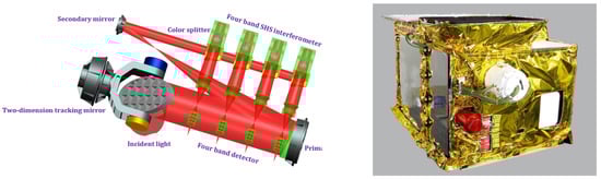
Figure 1.
Composition of the GMI payload optical system (left) and physical photos (right).
The ground data processing system obtains the greenhouse gas absorption spectrum data through data error correction, Fourier transform and other processing techniques performed on the interference image, and finally obtains the greenhouse gas column concentration results using the full physical inversion algorithm [13]. GMI’s working mode is set in advance, and it does not have the ability to judge land and sea in real time on orbit. After 14 days of continuous operation in the nadir mode, the sunglint mode works continuously for 7 days and the follow-up is carried out alternately according to this cycle. According to different ground sampling density requirements, the number of points taken in the rail crossing direction is divided into four modes: 1, 5, 7, and 9 points. The second mode is the sunglint observation mode, whichis used under ocean conditions and mainly calculates the flare tracking angle in real time in-orbit according to satellite, orbit, and other parameters and drives the scanning mirror to track. The working principle of the GMI load is shown in Figure 2, and the main technical indicators of the load are shown in Table 1.
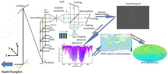
Figure 2.
The GMI’s workflow.

Table 1.
Main performance index of the GMI.
Before the GMI’s launch, a large amount of laboratory spectral and radiometric calibration work was carried out. The spectral calibration used the combination of an integrating sphere light source (SIRCUS) (as shown in Figure 3) with an external tunable laser and gas absorption method for fine calibration, and the spectral calibration accuracy reached 0.008 . In order to eliminate the influence of oxygen, carbon dioxide and water vapor in the air on the radiometric calibration accuracy, a nitrogen-filled circular replacement standard integrating the sphere radiation standard source (as is shown in Figure 4) was developed, which ensured that the integrating sphere was full of nitrogen without gas absorption and the payload absolute radiometric calibration was better than 4% [14].
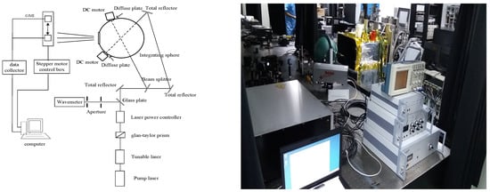
Figure 3.
Layout of the tunable laser hyperspectral scanning spectral calibration and the spectral calibration experiment.
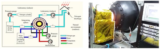
Figure 4.
Schematic diagram of the nitrogen circulation standard integrating sphere radiation source (left figure) and the radiation calibration experiment (right figure).
To improve the data accuracy, the GMI is equipped with an onboard calibration unit, as is shown in Figure 5, that uses high-stability sunlight as the calibration light source. The coordinate system is defined with X as the direction of satellite flight, Z as the direction of Earth observation and Y as the right-hand rule direction. When the GMI is going to carry out a calibration, the two-dimensional tracking mirror is adjusted from the nadir/sunglint observation mode to the calibration mode. The calibration is performed over the Antarctic. Firstly, the spectral calibration is carried out (the sunlight passes through the atmosphere, and the altitude is 10–100 km), and then the radiometric calibration is carried out (the sunlight does not pass through the atmosphere, and the altitude is greater than 100 km). To meet the requirements of in-orbit spectral and radiometric calibration, the calibration unit has a designed diffuser, light trap, ratio radiometer and other components, which are used to ensure the uniformity of the sunlight, monitor the decay of the diffuser and obtain the dark current of the instrument.
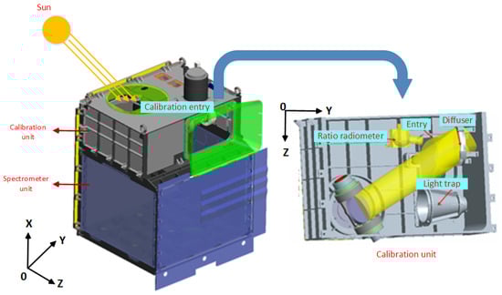
Figure 5.
Calibration unit of the GMI.
3. Screening Criteria
The calibration accuracy of the greenhouse gas payload plays an important role in the accurate inversion of greenhouse gasses. CO2 inversion of the data obtained from the Japanese greenhouse gas detection satellite GOSAT shows that there is a difference of 7–17 ppm between the inversion results and the model at the initial launch [15,16]. Obviously, such low accuracy cannot meet the design requirements. The National Environmental Agency of Japan (NIES), which is in charge of the inversion, believe that the instrument calibration result is one of the important factors affecting this result after analyzing this deviation; therefore, the calibration result is one of the keys to the application of remote sensing data [17]. When analyzing the whole process of the satellite remote sensor from its development and operation to the end of its mission, there are some problems that affect the application of remote sensing data, such as the inspection of sensor design indicators and changes in remote sensor performance during satellite operation. This process is inseparable from the calibration of satellite sensors. The laboratory absolute radiometric calibration can check the realization of the instrument indicators before the satellite remote sensor is launched and provide a basic basis for the subsequent application of remote sensing data. This calibration method is powerless to change the sensor performance during operation. By setting up a calibration system on the satellite platform, the sensor can be routinely calibrated during satellite operation to ensure the demand for calibration coefficients in remote sensing data applications. The key to this calibration method is the stability of the calibration source itself, so it is important to objectively evaluate it. Alternative calibration refers to the absolute radiometric calibration of the satellite remote sensor by carefully selecting the site, measuring the site and atmosphere and using radiative transfer calculations. This method can calibrate the satellite sensor in orbit on the basis of known accuracy, but it is impossible to perform regular calibration due to certain conditions.
Looking at the calibration methods for satellite sensors, the three existing calibration methods are independent of each other. In the whole cycle of satellite sensors from development to use, the undertakers play their respective roles. Effective satellite remote sensing data cannot be separated from the use of these methods. The satellite sensors need to be calibrated throughout the process. Site substitution calibration needs to be carried out synchronously during the period of greenhouse gas payload in orbit; however, it is necessary to solve the problem of the simultaneous measurement of environment and surface elements. A digital calibration field network can better solve such problems and improve the practicability of alternative calibration. By analyzing the GMI spectral principle, performance index and in-orbit operation mode, it can be concluded that the spatial resolution of the payload is about 10 km for non-imaging Earth observations, and that the spectral resolution is up to 0.035 nm [18]. However, the existing digital calibration field network is mainly designed for an imaging load with a meter-scale spatial resolution, which is quite different from the GMI field calibration application scenario. Data information acquisition of the digital calibration site is the key to determining whether the payload calibration can be achieved. In order to adapt to the high frequency of the orbit radiometric calibration requirements of the new greenhouse gas satellite load, achieve multisite high-frequency calibration without the support of measured data and better track the changes in the in-orbit radiation characteristics of remote sensors, it is vital to obtain basic data that can accurately describe these site characteristics. Based on the characteristics of the GMI, this section comprehensively considers the radiation site area, surface reflection characteristics, surface elevation characteristics, aerosol characteristics, greenhouse gas concentration and other factors, and screens the digital calibration radiometric correction field networks that meet the requirements of GMI alternative calibration on a global scale. The specific screening criteria are as follows:
(1) Site area: the effective area of the site is larger than the GMI field of view, and has good air terrain flatness so that during the radiometric calibration of the instrument, the impact of poor registration is minimized;
(2) Surface reflectance: the site has a high surface reflectance value and can obtain calibration observation data with a high signal-to-noise ratio. In addition, the surface reflectance should have good spatial uniformity and temporal stability;
(3) Atmosphere and meteorology: the site should mainly have sunny weather conditions, and the climate should be relatively stable throughout the year. The site atmospheric conditions are relatively simple, and the aerosol value is low;
(4) Greenhouse gas concentration: the greenhouse gas concentration of the site is relatively stable and is far away from cities, industrial areas and other carbon source areas, as well as forests, oceans and other carbon sink areas.
3.1. Surface Reflectivity
Since the diameter of the GMI is about 10.3 km, the calibration field should be continuous and uniform in space, and the length and width of the calibration field should be more than 10 km. Through an analysis of the global surface feature classification map, different large, continuous areas with uniform surface feature types are selected and analyzed on a global scale. In the process of actual site selection, it is found that only desert and vegetation types have large areas and continuous surfaces. Due to the limitations of these site areas, it is difficult to select a variety of surface types. In order to meet the requirement that the load detection data can obtain a high signal-to-noise ratio, it is also necessary to select a site with a high reflectivity value. Figure 6 shows the surface reflectance curves of different surface types in the four spectral channels of the GMI payload. Desert surfaces have high reflectance values. The subsequent site selection focuses on uniform desert surface areas.
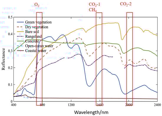
Figure 6.
Surface reflectivity curve of different surface feature types in the GMI spectral channel.
In addition to ensuring that the surface reflectivity has a high value, the stability of the surface reflectivity of the site should be considered in the process of selecting the site. At the same time, because the calibration field area selected by the GMI is large, the surface reflectivity of the site should be kept in a relatively uniform state. MYD09GA is a MODIS reflectivity product, with a day as the time resolution and a spatial resolution of 500 m. At the same time, the product has a corresponding longitude and latitude. This is convenient for matching the surface reflectivity of the corresponding site. The data on the statistical analysis of the surface reflectivity in this paper were obtained from the MODIS reflectivity product [19]. The coefficient of variation (CV) value can be used to analyze the uniformity of the reflectivity in the area to be studied. It is obtained by dividing the standard deviation of the reflectivity value in the area to be studied by the mean value. This equation is shown in Formula (1):
where s is the standard deviation of the surface reflectance of each pixel within the site, is the average value and the value is proportional to the degree of change. The smaller the value, the better the uniformity, and vice versa.
The variation coefficient of the site is calculated using Formula (1) to reflect the uniform reflectivity of each area within the site. The Kufra, Libya desert site obtained from the preliminary area screening is taken as the analysis object (this site is taken as an example for subsequent analysis). In 2018, a sunny day was selected from each month to analyze and calculate the variation coefficient of the surface reflectivity of the site. The CO2-1 spectral channel results are shown in Table 2. The variation coefficient of the surface reflectivity of the Kufra, Libya site is about 1%, which indicates that the surface reflectivity of each pixel in the site area changes little and has high uniformity.
Table 2.
CV of the Kufra, Libya field.
It can be seen from the analysis in Table 2 that the surface reflectance of each pixel in the Kufra, Libya site area shows little change, so the typical value of the surface reflectance of this calibration field can be characterized by the mean value method. The monthly average surface reflectivity of the Kufra, Libya site in 2018 is shown in Figure 7a. The annual average surface reflectivity is 0.5020, and the standard deviation is 0.2%. At the same time, in order to analyze whether the surface reflectivity of the Kufra, Libya site fluctuates significantly over short time periods, we also analyzed the surface reflectivity of July 2018 with many acquired day-by-day values. The statistical results are shown in Figure 7b and show a variance of 0.02%. The results show that the surface reflectivity of the Kufra, Libya site does not fluctuate significantly over short time periods.
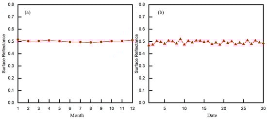
Figure 7.
(a) Surface reflectance of the Kufra, Libya site in 2018. (b) Surface reflectance of the Kufra, Libya site in July 2018.( red circle represents the monthly average result, red trangle represents the daily average results).
On the one hand, the stability of the surface reflectivity can be analyzed by a statistical analysis of the surface reflectivity data at different times; on the other hand, when the atmospheric environment is relatively stable, the stability of the calibration radiation characteristics of the calibration field can be analyzed by comparing the spectra of the GMI data at different observation points within the range of the calibration field at different times while excluding the influence of solar height. After the solar radiation reaches the surface through the atmosphere, it will be reflected to the instrument entrance pupil. The influencing factors of the reflection process are the surface reflectivity and the solar altitude angle. When the atmosphere is relatively consistent, the details can be expressed by the following formula:
where is the entrance pupil radiance, is the solar radiation, is the atmospheric transmittance, is the solar altitude angle and is the surface reflectance.
It can be seen from the above formula that the stability of the surface reflectivity can be evaluated when the radiance of the entrance pupil and the solar altitude angle are known. It is assumed that the radiance of the entrance pupil corresponding to two observation points at different times is expressed by the following formula:
so:
It can be inferred from Formula (4) that after removing the influence of the solar altitude angle of the observation point data, the reflectivity of the area to be studied can be evaluated by comparing the spectral data. Table 3 shows the basic information of the data from different observation points matched at different times at the Kufra, Libya site.
Table 3.
Data information of GMI observation points at Kufra, Libya site.
Figure 8 shows the comparison between the original spectral map (curves 1 and 2) of the data of the two observation points and the spectral data (curve 3) after excluding the influence of the solar altitude angle via Formulas (2–4). From the figure, it can be seen that after excluding the influence of the solar altitude angle, the spectra of the data of the two observation points are similar, indicating that the radiation characteristics of the Kufra, Libya site are stable and that the spectral data observed at different transit times are consistent (the maximum change rate is 3.1%).
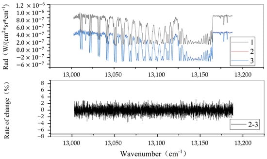
Figure 8.
Spectral stability analysis of the Kufra, Libya site in different observation periods.
3.2. Meteorological and Atmospheric Data
Weather conditions are the key factor affecting whether the site is suitable for carrying out the site calibration. Cloudy and rainy weather accompanied by dark clouds and rain will lead to the failure of the calibration task, so according to the site’s historical weather website (http://www.tianqihoubao.com/guoji/, accessed on 1 January 2018 to 1 December 2018), we statistically analyzed the stability and regularity of the weather conditions at the research site, determined whether the research site was suitable for carrying out the GMI site calibration task and identified a time period that was suitable for the calibration. A site with little continuous sunny weather should not be considered as a GMI calibration site. The results of the statistical analysis of the weather conditions of the Kufra, Libya calibration site in 2018 are shown in Figure 9.
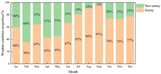
Figure 9.
Statistical chart of weather conditions at the Kufra, Libya site in 2018.
1. The site has fewer sunny days in the first half of the year, and the proportion of sunny days in April and May is only 43.33% and 45.16%, respectively;
2. The number of sunny days at the site increases significantly after June, accounting for more than 60% of days this month and more than 90% of days in August and September;
3. In 2018, the site had sunny weather in the first half of the year, and the number of days suitable for site calibration was less than that in the second half of the year. The number of sunny days was 246, accounting for 67.39% of the year. The statistical results show that the Kufra, Libya calibration site has a lot of sunny weather all year round, and the second half of the year is more suitable for the GMI to carry out site calibration.
During site calibration, radiation transfer between the space and the ground is realized through radiation transfer. The RTM we adopt in this study is SCIATRAN v3.5, which was developed by V.V. Rozanov and A.V. Rozanov [20] and adopted by GMI retrieval [6]. Aerosol optical depth (AOD) is an important parameter in the atmosphere. MODIS Terra (MOD04) and MODIS Aqua (MYD04) products can provide aerosol optical thicknesses of four spectral bands, 0.47 μm, 0.55 μm, 0.66 μm and 2.13 μm, respectively. Using 0.55, 0.66 and 2.13 μm aerosol products for wavelength interpolation, the aerosol optical thickness of four GMI spectral channels (0.76 μm, 1.575 μm, 1.65 μm, 2.05 μm) can be obtained. Figure 10 shows the monthly average statistical results of aerosol optical thickness (wavelength = 550 nm) in Kufra, Libya, Farafra, Egypt 1 and the Arabian Peninsula in 2018. The statistical results show that the aerosol content in the three sites is low, and there is no significant fluctuation in the aerosol content in different time ranges. Generally, AOD < 0.3, so the requirements for AOD content in site calibration were met.
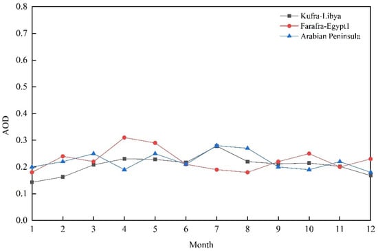
Figure 10.
Monthly average statistics of aerosol optical thickness of three sites in 2018.
Because the site calibration calculation needs to accurately calculate the theoretical simulation spectrum at the load entrance pupil, the greenhouse gas concentration in the radiation transfer calculation needs to be input into the model as an a priori value. If the regional greenhouse gas concentration in the calibration field fluctuates greatly, there will be some errors in the simulation spectrum, leading to large calibration coefficient errors. The digital calibration site of greenhouse gas load should be far away from areas of human activity so that the greenhouse gas concentration is only affected by seasonal fluctuations.
3.3. Digital Calibration Field Results
According to the above digital calibration field screening criteria, 14 radiation digital calibration fields, including Kufra, Libya, were selected globally. Due to the large field of view of the observation point, the lengths and widths of the selected sites are more than 15 km. Due to the limitations on site areas, the surface feature types are mainly desert types, and the site surface reflectance is between 0.3 and 0.8. The regional distribution of radiation calibration fields is shown in Figure 11, and the specific information of the calibration fields is shown in Table 4 and Table 5.
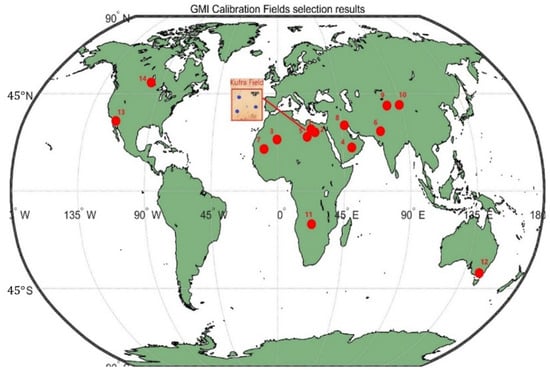
Figure 11.
GMI digital calibration field network selection results (red circles and numbers represent the calibration field and its serial number).
Table 4.
Statistics on the evaluation parameters of the GMI calibration field in 2018.
Table 5.
GMI radiation calibration field information.
4. Calibration Methodology
In order to further calculate the site calibration coefficient, it is necessary to match the location of GMI actual observation data with the location of the calibration field to ensure that the observation data for site calibration is included in the scope of the calibration field so as to ensure the correctness of the site calibration results. Due to the large field of view of the GMI and non-imaging of the ground, geometric processing should be performed on the data before calibration data matching, and reasonable matching results should be obtained by following certain matching principles.
4.1. Geometric Correction
The GMI is a non-imaging instrument, and the difference between the theoretical pointing position and the actual pointing position will cause observation error in the sudden change area of the ground. Therefore, before the observation data matches the calibration field, it is necessary to use the statistical analysis of the data to establish the relationship equation between the actual pointing and the theoretical pointing error to solve the longitude and latitude migration parameters and correct the longitude and latitude of the observation data to achieve the unity of observation and pointing. The premise of matching the actual calibration observation data with the effective site is to accurately align the GMI observation points. Due to the uniform geomorphology of the coastline area and the large difference in reflectivity between the land and the ocean surface, the average DN value of the interferograms of observation points on the ocean is much smaller than that on the land. When the average DN value of the observation point is the middle value, the point will fall on the coastline with a large probability. Therefore, the geometric position correction of GMI can be completed by using the characteristics of the observation point interference image. Figure 12 shows the flow chart of GMI geometric processing.
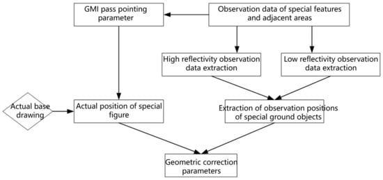
Figure 12.
GMI geometric processing flow chart.
The average luminance value of the baseline of the interferogram is set as DN1 on land and DN2 on sea, then the average luminance value I of the interferogram at the observation point of the coastline is calculated according to Formula (5):
where is the area of the observation point in a land area and is the area of the observation point in an ocean area. By determining that the observation point is a coastline point, the matching between the initial longitude and latitude of the observation point and the actual longitude and latitude is obtained. The longitude and latitude deviations were obtained by least-squares fitting. The longitude and latitude deviation formula was used to complete the pointing registration of the longitude and latitude of the GMI’s actual calibration observation point, which solves the problem of the geographic location information registration of the observation point caused by GMI non-Earth imaging.
According to the requirements for the selection of special features, the geometric calibration field of Durban, including the coastline, has been determined (Figure 13), and 100 GMI observation points within the site range have been selected for DN value reading and longitude and latitude reading, which are marked on the corresponding geometric location of the site; that is, the actual observation location of the observation points determines the GMI observation point located on the coastline. The longitude of the corresponding observation point is recorded as coastline point X, the latitude of the observation point is recorded as coastline point Y, the longitude of the intersection points between the GMI observation point and the coastline is recorded as offset X and the latitude of the intersection point is recorded as offset Y.
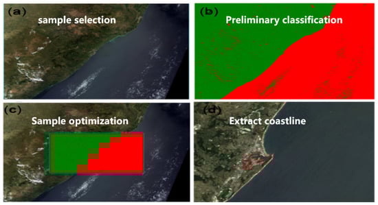
Figure 13.
Coastline extraction of Durban geometric calibration field.
The fitting formulas for longitude offset and latitude offset are obtained according to the fitting formula using the least-squares method, and the results are as follows:
4.2. Data Matching
The original data obtained by the GMI are in the form of an interferogram (Level 0) that was collected by an array detector. The radiance spectrum (Level 1) of the target gas was obtained through the processing techniques of error correction, Fourier transform, spectral calibration and radiation calibration performed on the satellite-downloaded detection data. The atmospheric inversion of spectral data based on the optimization iteration algorithm can yield the global column concentration distribution data for CO2 and CH4 (Level 2). This allows us to draw a global concentration map and estimate the global carbon flux (emission and source) (Level 3) and three-dimensional (3D) distribution of CO2 and CH4 after analyses that utilize the atmospheric transport model. The Level 0 data format is raw. The Level 1, Level 2 and Level 3 data formats are HDF5 format. The data products include not only scientific observation data but also satellite platform parameters, payload state parameters, calibration coefficients and other auxiliary data. This information is convenient for users to process the production of related scientific data products.
Because the load performance is easy to change at the initial stage of the launch, the site calibration calculation is carried out for three consecutive months (from September to November 2018) after the start of observations with the GF5-01 satellite GMI payload. The observation data are matched with the matching calibration field according to the longitude and latitude of the observation point. The central longitude and latitude and the length and width are known in the calibration field. The GMI observation data provide the central longitude and latitude and the 10 km diameter. To ensure the accuracy of the GMI site calibration data application, data matching should follow the following principles: before screening the observed data, the channel effectiveness should be determined to ensure that the corresponding channel spectral data can be read correctly; the observation points shall be completely included in the scope of the site to reduce the calibration error caused by the observation points falling outside the scope of the calibration field; when the observation point is within the scope of the site, we should ensure that there are no clouds above the observation point to avoid the impact of clouds.
According to the determined data-matching principles, effective observation data are matched using the following methods:
1. To judge the effectiveness of the observation data channel, a preliminary judgment should first be made according to the QualityFlag quality label provided in the GMI primary product, followed by a judgement as to whether the data with the quality label of “1” can be correctly read from the spectrum;
2. When the effective data are matched with the calibration field, in order to ensure that the observation point completely falls within the scope of the calibration field, the longitude and latitude of the observation point’s center should be included in the calibration site. The red dotted line in Figure 14 represents the boundary of the calibration field, and the green circle represents the observation point. The center of the observation point must fall inside the boundary line to be considered valid calibration data.
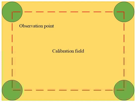
Figure 14.
Position relationship between observation point and calibration field.
3. When the above two conditions are met, according to the corresponding time of the observation point, one should query whether there is cloud coverage according to DPC cloud product [21,22]. Similarly to POLDER, the DPC instrument consists of three principal components: wide-field telecentric optics, a rotating wheel carrying the polarizers and spectral filters and a digital camera with a 512 × 512 pixel CCD detector. The wide-field telecentric optics and CCD matrix yield a field of view of ±50° both along the track and cross-track, and the pixel size is 3.3 km at nadir under a swath width of 1850 km. The GMI center is matched outward by 3 × 3 DPC pixels, and the DPC scanning width is large enough to ensure space-time consistency (Figure 15). If there is a large area of cloud coverage, the data cannot be used for site calibration.
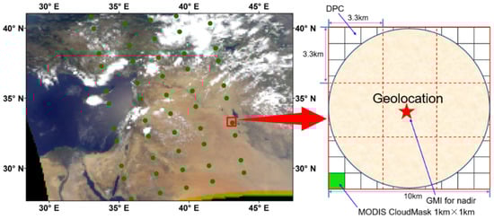
Figure 15.
Schematic diagram of GMI, DPC and MODIS data space matching.
Based on the established data-matching principle, the effective observation data of each channel of GMI is screened within the 14 effective calibration fields obtained, meeting the requirements for GMI to carry out site calibration. The matched observation data lay the foundation for the next step of site calibration coefficient calculation. Table 6 shows the matching quantity of the observation data of a calibration field with an area of 100 km × 100 km in Kufra, Libya, Fafara, Egypt 1 and the Arabian Peninsula. The detector type and dynamic range adopted by the four spectral channels of GMI are different. CCD (O2), InGaAs (CO2-1, CH4) and MCT (CO2-2) are selected, respectively, so the effective data amount of each spectral channel is different.
Table 6.
Calibration data of the GMI.
4.3. Calibration Coefficient
The GMI was developed based on spatial heterodyne interference technology, and its spectral resolution is extremely high. Therefore, in the process of site calibration, it is necessary to use a high-precision hyperspectral radiation transfer model to simulate the instrument’s entrance pupil radiance spectrum at the observation time of the calibration field, according to the surface characteristic parameters and atmospheric environment parameters (See Figure 16). The working band of the SCIATRAN radiative transfer model is from ultraviolet to near-infrared, and the spectral resolution also meets the requirements for a simulated spectrum in GMI site calibration. During the calculation of the GMI site calibration coefficient, the surface reflectivity, atmospheric parameter information and auxiliary parameters of the calibration observation data (observation geometry, platform parameters, time, etc.) of the calibration site must first be obtained using MODIS data products, and then this information must be input into the high-precision radiative transfer calculation model SCIATRAN after preprocessing to calculate the radiance data at the entrance pupil of the ultra-high spectrum. The spectral radiance at the entrance pupil is convolved with the instrument linear function of the corresponding channel of the load, and finally the simulated spectrum is obtained.
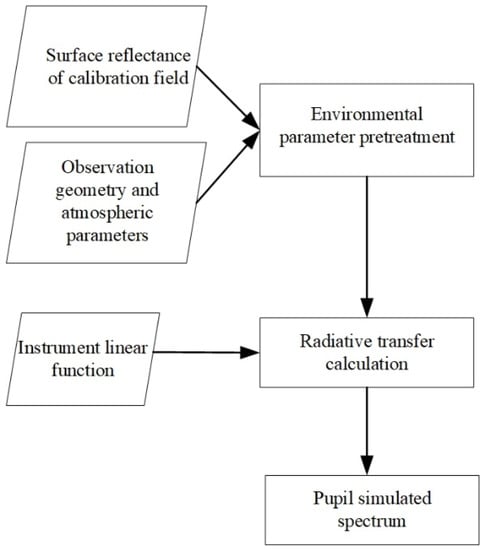
Figure 16.
Flow chart of simulated spectrum calculation.
The radiance spectrum of GMI observation data is directly read from the GMI primary products, which are in HDF5 format. The radiance spectrum is obtained mainly by reading three labels: SpectraData (restored spectral data), RadioCaliCoeff (radiation calibration coefficient) and SpecCaliCoeff (spectral calibration coefficient). The radiance of the observed number spectrum is obtained by calculating the recovered spectral data and the radiometric coefficient after laboratory calibration, as is shown in Formula (8):
The traditional calculation method for the radiometric calibration coefficient of an imaging sensor mainly uses the radiation transfer model to simulate the instrument’s entrance pupil radiance, and then calculates the calibration coefficient by correlation with the average DN brightness value of the actual observation image. When the load observes the calibration field, the DN brightness value of the observed image of the corresponding band and the simulated theoretical pupil radiance should be obtained, and the least-squares method used to obtain the slope and intercept of the radiometric calibration of the remote sensor, as is shown in Formula (9):
where is the calibration slope, is the calibration intercept, and is the equivalent radiance of the corresponding band of the remote sensor.
For spectral-type greenhouse gas satellite load observation data, the method of determining the baseline within the spectral range can reflect the in-orbit operation of the load well. Figure 17 (left) shows the spectrum range of the O2 channel and the actual spectrum range of the GMI observation data. Figure 17 (right) shows the spectrum range of the CO2-1 channel and the actual spectrum range of the GMI observation data. Because the corresponding spectral range of the GMI actual observation channel is narrow and the spectral absorption is rich, it is difficult to determine the baseline within the GMI observation spectral range to calculate the site calibration coefficient.
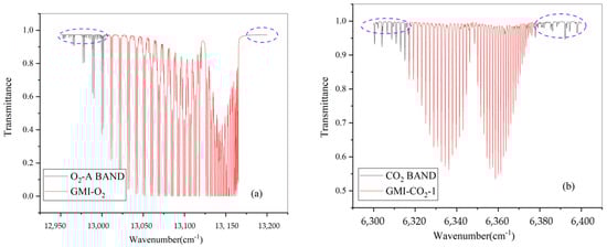
Figure 17.
Spectral range of the O2 (a) and CO2-1 (b) channels.
Neither the calculation method of the site calibration coefficient of the traditional imaging instrument nor the spectral baseline calculation method is applicable to the GMI, so this section will calculate the site calibration coefficient by analyzing the main gas collection of the corresponding band of the four channels of the GMI and selecting the wavelength points that have lower absorption rates of other gases in the band range that can directly reflect the in-orbit performance of the instrument. The O2 channel is mainly affected by O2 and O3. The range of the CO2-1 channel is mainly affected by H2O and CO2. The range of the CH4 channel is mainly affected by H2O, CO2, and CH4. The CO2 channel is mainly affected by H2O, CO2, and CH4. The calibration site is a clean area with a greenhouse gas background that is far away from any industrial building areas, with no interference and no external input. This is so that the stability of the gas in the calibration field in maintained. As is shown in Figure 18, the transmissivity of the main gas in each of the four channels of the GMI is calculated via the radiation transfer model to reflect the absorption of the gas in the band. Different wavelengths have different degrees of absorption of different gas components. The corresponding transmissivity of each wavelength point is superimposed to calculate the total transmissivity of each wavelength point. The wavelength point with the smallest impact on the absorption should have the largest corresponding total transmissivity, excluding the external impact of atmospheric component absorption, which can best reflect the radiation performance of the instrument itself and can be used as the wavelength point for the calculation of the calibration coefficient of the research site.
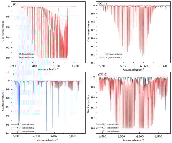
Figure 18.
Main gas permeability of the four GMI channels.
According to the gas absorption in the band, the wave number points with non-absorption or small absorption effects in each channel were determined, and the results are shown in Table 7.
Table 7.
Results of the four GMI channels’ unabsorbed wavenumbers.
5. Calibration Results
Selecting the calibration data of a single calibration site to calculate the site calibration coefficient may lead to large errors. Therefore, it is necessary to calculate the site calibration coefficient of the instrument through multiple effective observation data of the site, eliminate obvious unreasonable result values and obtain the site calibration coefficient within a certain period of time at the calibration site using fitting calculations to characterize the site calibration coefficient of the instrument. The site calibration coefficient results of the CO2-1 channel from the observed data that meet the site calibration conditions during the three months from September to November 2018 at the Kufra, Libya site are shown in Figure 19. The ordinate is the radiance value of the non-absorbable wave number corresponding to the measured spectrum of the observed data (6314.25/6352.65/6376.35 cm−1), and the abscissa is the radiance value of the wave number corresponding to the simulated spectrum of the SCIATRAN model radiation transfer calculation at the corresponding observation time. Fitting different points in the figure can help us to avoid the random error of a single point when calculating the site calibration coefficient. The calculation results show that the site calibration coefficient of the CO2-1 channel at the Kufra, Libya site is about 1.0632 during the three months from September to November 2018, reflecting the good in-orbit operation of the GMI and almost no attenuation of the radiation performance.
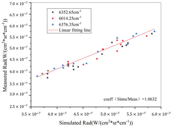
Figure 19.
Calculation of site calibration coefficient of the CO2-1 channel at the Kufra, Libya site.
According to the calculation method of the GMI site calibration coefficient combined with the GMI data matching results in Section 3, the effective observation data within the time range from September to December 2018 are obtained, and the time series site calibration results of different channels of GMI are statistically analyzed to monitor the attenuation changes in each channel during the in-orbit operation of the load. For a channel with a large attenuation, the calibration coefficient should be corrected to improve the product accuracy of the observed spectral data and ensure data stability during the long-term in-orbit operation of the load. The calculation results of the calibration coefficients of each spectral channel are shown in Figure 20.
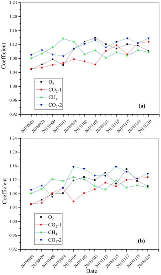
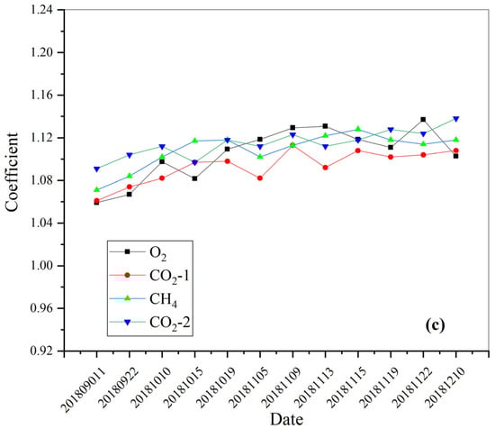
Figure 20.
GMI site calibration coefficient results. (a) Kufra, Libya, (b) Fafara, Egypt 1, (c) Arabian Peninsula.
The statistical results of the effective site calibration coefficient of the GMI channel are as follows: the range of the site calibration coefficient of the O2 channel is 1.05–1.15, the average value is 1.10 and the standard deviation is 2.72%. The calibration coefficient of the CO2-1 channel site is 1.05–1.13, the mean value is 1.09 and the standard deviation is 2.64%. The calibration coefficient range of the CH4 channel site is 1.08–1.10, the average value is 1.11 and the standard deviation is 2.73%. The calibration coefficient range of the CO2-2 channel site is 1.09–1.14, the average value is 1.12 and the standard deviation is 2.93%. The above results indicate that site calibration for the GMI should be carried out within a certain time range. The GMI can monitor the radiation performance attenuation of each channel in this period of time and modify the remote sensing data to a certain extent according to the site calibration coefficient.
6. Discussion
In order to verify the GMI site calibration results, the international high-precision greenhouse gas detection load of the GOSAT, which is of the same type, was used for cross-validation. The reliability of the site calibration coefficient was verified by comparing the difference between the radiance spectrum of the corresponding channel of the GMI before and after the application of the site calibration coefficient and the radiance spectrum observed by the GOSAT. That is, there is a certain difference between the GMI observation spectrum before the site calibration and the GOSAT observation spectrum. The GMI observation spectrum after correction with the site calibration coefficient is compared with the GOSAT observation spectrum. If the difference is reduced, the site calibration coefficient is considered to improve the accuracy of the GMI observation data to a certain extent. Otherwise, it indicates that there may be a problem with the calculation of the site calibration coefficient.
The GOSAT data mainly consist of the following levels: L0, FTS-L1A, FTS-SWIR L1B, FTS-TIR L1B, CAI L1B, FTS-SWIR L2, CAI L2, FTS-SWIR L3 and CAI L3 products. This article mainly uses the downloadable FTS L1B data from the official website of the GOSAT (https://data2.gosat.nies.go.jp, accessed on 1 November 2018). The product data are mainly GOSAT spectral data after phase correction, inverse Fourier transform, radiometric calibration, spectral calibration and geometric calibration. By downloading and processing the FTS L1B data products, the GOSAT observation spectra required for cross validation can be obtained. Figure 21 shows the observed spectrum of the GOSAT Band2 read from the FTS L1B data. The spectral range of the GOSAT Band2 channel is 5800 cm−1–6400 cm−1, and the spectral range of the GMI CH4 channel is 6317 cm−1–6377 cm−1. The spectral range of the GOSAT channel is much wider than that of the corresponding GMI channel. The spectral range of the GOSAT channel includes the complete spectral range of the corresponding channel of the GMI. Therefore, the GOSAT observation spectrum and GMI observation spectrum can be used for cross-validation.
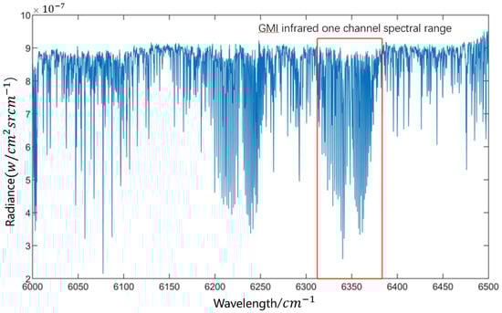
Figure 21.
The GOSAT L1B-Band2 observed spectrum.
In Table 8, the observation data in the Kufra, Libya calibration field on 11 October 2018 and the observation data of the GOSAT at the same time and in the same region are shown. According to the calculation method of the GMI site calibration coefficient in the previous section, the calibration coefficient of the Kufra, Libya calibration field is 1.0512. In order to conduct a validity judgment of the coefficient, the GMI observation data of the site will be used for analysis and judgment before and after the application of the site calibration coefficient and the GOSAT observation spectrum for cross-validation.
Table 8.
Cross-validation data information.
Figure 22 shows a comparison chart before the application of the site calibration coefficient of the GMI observation spectrum, and Figure 23 shows the comparison chart after the application of the site calibration coefficient of the GMI observation spectrum.
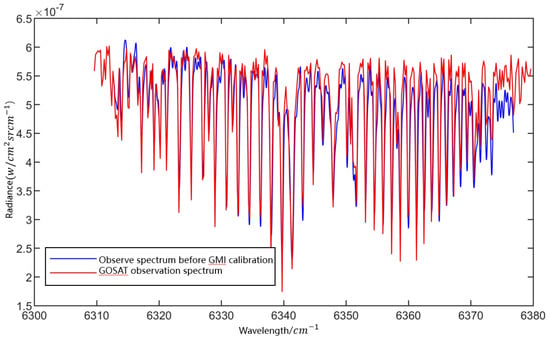
Figure 22.
The observed spectrum and the GOSAT spectrum before the GMI calibration.
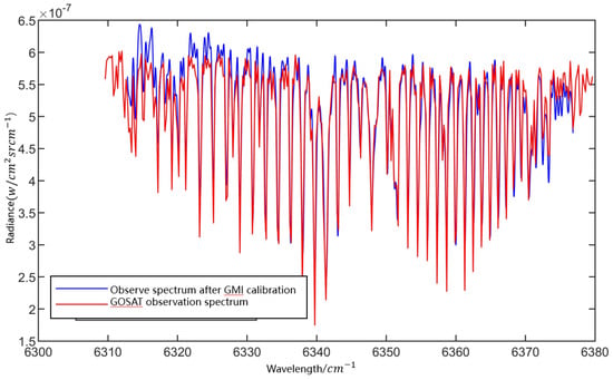
Figure 23.
The observed spectrum and the GOSAT spectrum after the GMI calibration.
In Figure 24 and Figure 25, the GMI observation spectrum is further compared with the GOSAT observation spectrum before and after the site calibration coefficient is applied by calculating the radiance ratio of the corresponding wave number of the GMI and GOSAT observation spectra. The calculated radiance ratio is obtained and fitted. The slope of the fitting line of the radiance ratio of the observed spectrum before the GMI calibration and the observed spectrum of the GOSAT is 0.928. The slope of the straight fit line of the radiance ratio between the observed spectrum after the GMI calibration and the observed spectrum of the GOSAT is 0.968. Through comparison, it was found that after the site calibration of the GMI observation spectrum, the observation spectrum is closer to the GOSAT observation spectrum than before the calibration, which shows that the calculation method and results of the site calibration coefficient are scientific and accurate.
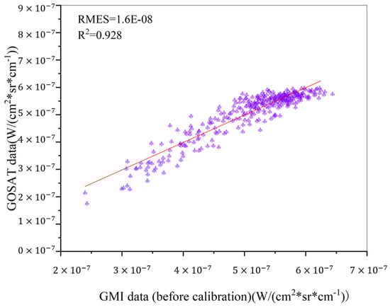
Figure 24.
The ratio of the observed spectrum and the GOSAT spectral radiance before the GMI calibration (purple symbols represents the observed data before calibration).
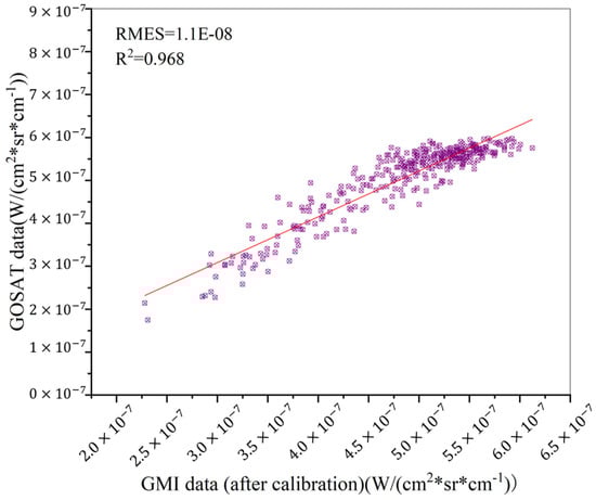
Figure 25.
The ratio of the observed spectrum and the GOSAT spectral radiance after the GMI calibration (purple symbols represents the observed data after calibration).
7. Conclusions
The GMI is a spatial interferometric greenhouse gas payload with a large field of view that is non-imaging and hyperspectral. It is mainly used to obtain global greenhouse gas (CO2 and CH4) column concentrations. In order to further improve the quantification accuracy of load remote sensing data products and ensure the reliability of inversion results, laboratory calibration and on-board calibration of this instrument have been carried out and actual data products have been successfully obtained. Based on the previous calibration work carried out on the GMI, this paper studies the site calibration of the load and introduces how to evaluate and select the calibration field and screen and match the actual observation data and the calibration field according to the large-field-of-view characteristic of the load of the station. We calculated the site calibration coefficient using the radiance value of the non-absorbable wave number points, and the reliability of the calibration results was verified through the GOSAT observation spectrum and the GMI site calibration coefficient before and after the application of the observation spectrum. Finally, site calibration was carried out at different times, at different calibration sites and with different calibration data; the results of the GMI site calibration coefficients from September 2018 to December 2018 were obtained, and the GMI in-orbit operation status was analyzed.
Author Contributions
Conceptualization, X.W.; Data curation, H.L.; Formal analysis, Z.L.; Funding acquisition, W.X.; Investigation, H.Y.; Methodology, H.Y.; Project administration, W.X.; Resources, H.S.; Software, H.Y.; Supervision, H.S.; Validation, Z.L.; Writing—original draft, H.S.; Writing—review & editing, H.S., Z.L. All authors have read and agreed to the published version of the manuscript.
Funding
This research was funded by Key deployment projects of Chinese Academy of Sciences (ZDRW-KT-2020-3).
Data Availability Statement
Restrictions apply to the availability of these data. GF-5 GMI Data was obtained from CRESDA and are available [http://www.cresda.com/CN/] with the permission of CRESDA.
Conflicts of Interest
The authors declare no conflict of interest.
References
- Schuh, A.E.; Byrne, B.; Jacobson, A.R.; Crowell, S.M.R.; Deng, F.; Baker, D.F.; Johnson, M.S.; Philip, S. On the role of atmospheric model transport uncertainty in estimating the Chinese land carbon sink. Nature 2022, 603, E13–E14. [Google Scholar] [CrossRef] [PubMed]
- Kuze, A.; Suto, H.; Nakajima, M.; Hamazaki, T. Thermal and near infrared sensor for carbon observation Fourier-transform spectrometer on the Greenhouse Gases Observing Satellite for greenhouse gases monitoring. Appl. Opt. 2009, 48, 6716–6733. [Google Scholar] [CrossRef] [PubMed]
- Miller, C.E.; Crisp, D.; DeCola, P.L.; Olsen, S.C.; Randerson, J.T.; Michalak, A.M.; Alkhaled, A.; Rayner, P.; Jacob, D.J.; Suntharalingam, P.; et al. Precision requirements for space-based data. J. Geophys. Res. Atmos. 2007, 112, D10314. [Google Scholar] [CrossRef]
- Hong, X.; Zhang, P.; Bi, Y.; Liu, C.; Sun, Y.; Wang, W.; Chen, Z.; Yin, H.; Zhang, C.; Tian, Y.; et al. Retrieval of Global Carbon Dioxide from TanSat Satellite and Comprehensive Validation with TCCON Measurements and Satellite Observations. IEEE Trans. Geosci. Remote Sens. 2022, 60, 3066623. [Google Scholar] [CrossRef]
- Shi, H.; Li, Z.; Ye, H.; Luo, H.; Xiong, W.; Wang, X. First Level 1 Product Results of the Greenhouse Gas Monitoring Instrument on the GaoFen-5 Satellite. IEEE Trans. Geosci. Remote Sens. 2021, 59, 899–914. [Google Scholar] [CrossRef]
- Ye, H.; Shi, H.; Li, C.; Wang, X.; Xiong, W.; An, Y.; Wang, Y.; Liu, L. A Coupled BRDF CO2 Retrieval Method for the GF-5 GMI and Improvements in the Correction of Atmospheric Scattering. Remote Sens. 2022, 14, 488. [Google Scholar] [CrossRef]
- Rayner, P.J.; O’Brien, D.M. The utility of remotely sensed CO2 concentration data in surface source inversions. Geophys. Res. Lett. 2001, 28, 175–178. [Google Scholar] [CrossRef]
- Sakuma, F.; Bruegge, C.; Rider, D.; Brown, D.; Geier, S.; Kawakami, S.; Kuze, A. OCO/GOSAT preflight cross-calibration experiment. IEEE Trans. Geosci. Remote Sens. 2010, 48, 585–599. [Google Scholar] [CrossRef]
- Crisp, D.; Eldering, A.; Gunson, M.R. Preliminary Results from the NASA Orbiting Carbon Observatory-2 (OCO-2). AGU Fall Meeting Abstr. 2014, 2014, A52E-01. [Google Scholar]
- CEOS LandNet Sites. Available online: http://calvalportal.ceos.org/ceos-landnet-sites (accessed on 1 November 2018).
- Bacour, C.; Briottet, X.; Bréon, F.-M.; Viallefont-Robinet, F.; Bouvet, M. Revisiting Pseudo Invariant Calibration Sites (PICS) Over Sand Deserts for Vicarious Calibration of Optical Imagers at 20 km and 100 km Scales. Remote Sens. 2019, 11, 1166. [Google Scholar] [CrossRef]
- Roesler, F.L.; Harlander, J.M. Spatial heterodyne spectroscopy: Interferometric performance at any wavelength without scanning. In Optical Spectroscopic Instrumentation and Techniques for the 1990s: Applications in Astronomy, Chemistry, and Physics; SPIE: Las Cruces, NM, USA, 1990; Volume 1318, pp. 234–243. [Google Scholar]
- Ye, H.; Wang, X.; Wu, S.; Li, C.; Li, Z.; Shi, H.; Xiong, W. Atmospheric CO2 Retrieval Method for Satellite Observations of Greenhouse Gases Monitoring Instrument on GF-5. J. Atmos. Environ. Opt. 2021, 16, 231–238. [Google Scholar]
- Xiong, W. Hyperspectral Greenhouse Gases Monitor Instrument (GMI) for Spaceborne Payload. Spacecr. Recovery Remote Sens. 2018, 39, 14–24. [Google Scholar]
- Yoshida, Y.; Ota, Y.; Eguchi, N.; Kikuchi, N.; Nobuta, K.; Tran, H.; Morino, I.; Yokota, T. Retrieval algorithm for CO2 and CH4 column abundances from short-wavelength infrared spectral observations by the Greenhouse gases observing satellite. Atmos. Meas. Tech. 2011, 4, 717–734. [Google Scholar] [CrossRef]
- Kataoka, F.; Crisp, D.; Taylor, T.E.; O’Dell, C.W.; Kuze, A.; Shiomi, K.; Suto, H.; Bruegge, C.; Schwandner, F.M.; Rosenberg, R.; et al. The Cross-Calibration of Spectral Radiances and Cross-Validation of CO2 Estimates from GOSAT and OCO-2. Remote Sens. 2017, 9, 1158. [Google Scholar] [CrossRef]
- Morino, I.; Uchino, O.; Inoue, M.; Yoshida, Y.; Yokota, T.; Wennberg, P.O.; Toon, G.C.; Wunch, D.; Roehl, C.M.; Notholt, J.; et al. Preliminary validation of column-averaged volume mixing ratios of carbon dioxide and methane retrieved from GOSAT short-wavelength infrared spectra. Atmos. Meas. Tech. 2011, 4, 1061–1076. [Google Scholar] [CrossRef]
- Wei, X. Greenhouse gases Monitoring Instrument(GMI) on GF5 satellite(invited). Infrared Laser Eng. 2019, 48, 24–30. [Google Scholar]
- MODIS Data Web. Available online: http://modis.gsfc.nasa.gov/ (accessed on 1 November 2018).
- Rozanov, V.V.; Dinter, T.; Rozanov, A.V.; Wolanin, A.; Bracher, A.; Burrows, J.P. Radiative transfer modeling through terrestrial atmosphere and ocean accounting for inelastic processes: Software package SCIATRAN. J. Quant. Spectrosc. Radiat. Transf. 2017, 194, 65–85. [Google Scholar] [CrossRef]
- Shen, F.; Zhang, Q.; Ma, J.; Li, Z.; Hong, J. Identification of polluted clouds and composition analysis based on GF-5 DPC data. J. Quant. Spectrosc. Radiat. Transf. 2021, 263, 107659. [Google Scholar] [CrossRef]
- Li, J.; Ma, J.; Li, C.; Wang, Y.; Hong, J. Multi-information collaborative cloud identification algorithm in Gaofen-5 Directional Polarimetric Camera imagery. J. Quant. Spectrosc. Radiat. Transf. 2020, 261, 107439. [Google Scholar] [CrossRef]
Disclaimer/Publisher’s Note: The statements, opinions and data contained in all publications are solely those of the individual author(s) and contributor(s) and not of MDPI and/or the editor(s). MDPI and/or the editor(s) disclaim responsibility for any injury to people or property resulting from any ideas, methods, instructions or products referred to in the content. |
© 2023 by the authors. Licensee MDPI, Basel, Switzerland. This article is an open access article distributed under the terms and conditions of the Creative Commons Attribution (CC BY) license (https://creativecommons.org/licenses/by/4.0/).