Automatic Detection of Subglacial Water Bodies in the AGAP Region, East Antarctica, Based on Short-Time Fourier Transform

Abstract

Subglacial water bodies are critical components in analyzing the instability of the Antarctic ice sheet. Their detection and identification normally rely on geophysical and remote sensing methods such as airborne radar echo sounding (RES), ground seismic, and satellite/airborne altimetry and gravity surveys. In particular, RES surveys are able to detect basal terrain with a relatively high accuracy that can assist with the mapping of subglacial hydrology systems. Traditional RES processing methods for the identification of subglacial water bodies mostly rely on their brightness in radargrams and hydraulic flatness. In this study, we propose an automatic method with the main objective to differentiate the basal materials by quantitatively evaluating the shape of the A-scope waveform near the basal interface in RES radargrams, which has been seldom investigated. We develop an automatic algorithm mainly based on the traditional short-time Fourier transform (STFT) to quantify the shape of the A-scope waveform in radargrams. Specifically, with an appropriate window width applied on the main peak of each A-scope waveform in the RES radargram, STFT shows distinct and contrasting frequency responses at the ice-water interface and ice-rock interface, which is largely dependent upon their different reflection characteristics at the basal interface. We apply this method on 882 RES radargrams collected in the Antarctic’s Gamburtsev Province (AGAP) in East Antarctica. There are 8822 identified A-scopes with the calculated detection value larger than the set threshold, out of the overall 1,515,065 valid A-scopes in these 882 RES radargrams. Although these identified A-scopes only takes 0.58% of the overall A-scope population, they show exceptionally continuous distribution to represent the subglacial water bodies. Through a comprehensive comparison with existing inventories of subglacial lakes, we successfully verify the validity and advantages of our method in identifying subglacial water bodies using the detection probability for other basal materials of theoretically the highest along-track resolution. The frequency signature obtained by the proposed joint time–frequency analysis provides a new corridor of investigation that can be further expanded to multivariable deep learning approaches for subglacial and englacial material characterization, as well as subglacial hydrology mapping.

1. Introduction

The subglacial environment and activities in Antarctica have an important effect on global climate change and sea level rising [1]. Large collections of subglacial water bodies can affect the overlaying internal icesheet structure, rheology of the ice body [2], and can also modulate velocities of ice streams and outlet glaciers [3]. Some subglacial water bodies connect over large distances through complex hierarchical hydrological chains [4,5]. The increasing evidence of a well-connected subglacial drainage system in Antarctica indicates that the subglacial hydrologic system is indispensable in understanding the mass balance of Antarctic ice sheets and its responses to global sea-level change [3].

Over the years, abundant methods have been developed and employed to discover the subglacial hydrology systems, and to reveal the underlying mechanism of how various drivers such as geothermal heat and basal friction increase the basal melting of the Antarctica ice sheet, accelerating the formation of channels of subglacial water bodies and drainage systems [6,7,8,9]. In particular, subglacial water bodies, or accumulated lakes entrapped beneath the ice sheet, are crucial elements for the subglacial hydraulic network environment and water circulation. Since the discovery of subglacial lakes near the Russian Soviet Station using radio echo sounding (RES) by Robin et al. [10], significant progress has been made in the study of Antarctic subglacial water bodies over the past 50 years, aided by various geophysical and remote sensing technologies, with the onboard platform ranging from terrestrial, to airborne [8], and even satellite [11]. The fourth inventory of Antarctica subglacial lakes was released in 2012, identifying 379 subglacial lakes [12]. As of February 2022, there are 773 subglacial lakes in the global inventory, of which 675 are from Antarctica, 64 are from Greenland, two are from the Devon Ice Cap, six are under the Icelandic ice cap, and 26 are from glaciers in valleys [13].

In general, subglacial lakes can be classified into two main types, i.e., an “active lake” [14,15,16] and a “stable lake” [17,18,19]. The former has periodic water exchange, which can be identified by the surface elevation change measured during repeated elevation observations, whereas the latter has characteristics that can be readily identified by using RES surveys [20]. In a typical airborne RES survey, the radar sounder emits low-frequency radar waves and the reflection power from the subsurface is recorded along a two-way travel time, which forms a one-dimensional A-scope. Discrete A-scopes along the survey line are assembled to construct a two-dimensional B-scope or radargram [20]. Since the reflection at the ice–water interface is stronger than that of the ice–rock interface, assuming similar specular conditions [21,22], the bed return power is often used as the major quantitative differentiator for basal materials, where stable lakes can be further classified into several subgroups, such as definite lakes, dim lakes, fuzzy lakes, indistinct lakes, and failing lakes [17]. Visually, a subglacial lake in the radargram can be described as a continuous basal reflection of 500 m or more, over which the water would be in a hydrostatic equilibrium [17]. However, due to the uncertainty of englacial attenuation, the identification of subglacial water bodies by such a sole examination of the bed return power has been demonstrated to be insufficient.

To avoid the subjective influence of the human estimate and make a quantitative judgment, manual and semiautomatic methods have been widely developed [23,24,25,26,27,28,29,30], and various parameters have been proposed to quantify the difference between the ice–water and ice–bedrock interfaces, such as the relative echo strength, specularity content, reflection coefficient, and cross-track bed energy [31,32]. These parameters have provided an effective tool for the automatic batching and identification of subglacial water bodies in RES data. However, the selected feature dimension is still often insufficient, which is, therefore, difficult to adapt to complex and diverse subglacial terrain conditions. On the other hand, these methods often focus on certain index calculations that rely on the magnitude of the absolute or relative intensity of the radar echoes, supplemented by parameters such as topography, hydraulic potential, and roughness, which complicates the reflection and scattering of RES signals [31,33,34,35,36,37]. More recently, Ilisei et al. [38] proposed a novel machine learning approach to discriminate between the lake and nonlake radar reflections based on the extracted three features (i.e., the basal topography, the shape of the basal reflected waveforms, and the statistical properties of the basal signal). In particular, the different shapes of the A-scope waveforms for the ice–water and ice–rock interfaces provide an intriguing representation of the physical behaviors of the incident, reflection, and scattering waves at the basal interface. They greatly improve the detectability of subglacial water bodies at a fine spatial resolution since the proposed pattern recognition approach is implemented at the A-scope level, which inherently means the highest possible resolution.

The majority of these aforementioned methods for subglacial water detection are from the perspective of the data processing of time-domain signal waveforms, which ignores the inherent frequency characteristics of the A-scope waveforms. In this study, we propose to utilize the short-time Fourier transform (STFT), a joint time–frequency analysis (JTFA) method, to analyze the inherent frequency characteristics of each A-scope of the RES data in Antarctica, which serves as the main contribution of this paper. Note that STFT has been widely used to evaluate the frequency characteristics of a time-series signal [39]. It can also extract the peak frequency in the spectrograms at a particular time/depth and generate a slice view of these peak frequencies that can reveal the location of subsurface targets. In addition, STFT is very easy to implement, which serves as a good illustrative JTFA method for the current study. It is successfully demonstrated to be able to help to differentiate between two major basal materials, i.e., subglacial water bodies and bedrocks, by using the publicly available RES data from the Antarctic’s Gamburtsev Province (AGAP) region, and it is compared with the recent inventories of subglacial lakes [13] and water bodies [29].

In Section 2, the basic characteristics of the basal interface are described, which lay the foundation of the proposed STFT-based method for differentiating subglacial water bodies and bedrocks, as detailed in Section 3. In Section 4, the detection results of the subglacial water bodies within the AGAP region in East Antarctica are provided for typical B-scopes, followed by the creation of a distribution map of subglacial water bodies in the AGAP region. Finally, conclusions are drawn in Section 5.

2. Characteristics of the Basal Interface

The traditional visual interpretation of subglacial water is largely dependent upon the characteristics of the basal interface in the RES data, which can be mainly characterized as being hydraulically flat and brighter than the surroundings in terms of reflected radar power. The former characteristic is based on the fact that subglacial water normally flows down the gradient of hydraulic heads and ponds in hydraulically flat regions, where the hydraulic flatness condition is satisfied [40]. Furthermore, if such flatness is characterized from the perspective of the radar wavelength, it means that subglacial water bodies shall have an interfacial roughness comparable or larger than that of the radar wavelength of the RES system [17]. The second characteristic is mainly based on the radar reflection intensity at the interface between ice and various basal materials, which can include water, rocks, and sediments, etc. [21]. Relative dielectric permittivity (${\epsilon }_r={\epsilon }^{\prime }-j{\epsilon }^{″}$) and electrical conductivity ($\sigma$) are used to describe their basic geophysical properties and response to radar waves. The real part of the permittivity of basal materials varies from about 4 to 81, as compared to that of overlain ice of about 3.15. The imaginary part, which includes the frequency-dependent loss component, is often difficult to determine, but the conductivity ${\sigma }_b$ is believed to be in the range of 0.01 mS/m to 3000 mS/m, as compared to the overlain ice (${\sigma }_i\approx$ 0.01 mS/m) [38]. When the radar waves reach the ice–water interface, due to the high permittivity of water (${\epsilon }_{\mathrm{rw}}$ ≈ 81) [41], most of the radar waves are reflected, as the calculated reflection coefficient $\rho$ is large when using Equation (1), where ${\epsilon }_{rb}$ is the relative permittivity of the basal material (e.g., ${\epsilon }_{rw}$ for water and ${\epsilon }_{rr}$ for bedrock), and ${\epsilon }_{ri}$ is the relative permittivity of ice. Only a very small amount of energy crosses the interface into the water, thus producing a sharp reflection signature in the A-scope [36]. As a result, a typical A-scope waveform for the ice–water interface shall have a high peak power, accompanied with steep leading and trailing edges [38], as illustrated by the red A-scope in Figure 1b. With the first characteristic of hydraulic flatness, which refers to a high degree of correlation of such sharp waveforms with adjacent along-track A-scopes, one can visually see in Figure 1a the subglacial water body as a flat interface in the along-track direction and as a narrow interface in the range direction.

$$\rho =\left|\frac{\sqrt{{\epsilon }_{rb}}-\sqrt{{\epsilon }_{ri}}}{\sqrt{{\epsilon }_{rb}}+\sqrt{{\epsilon }_{ri}}}\right|$$

(1)

On the other hand, bedrocks or dry basal materials do not have a high permittivity (e.g., ${\epsilon }_{\mathrm{rr}}$ ≈ [10 30] for bedrocks) [21], and thus, they will not lead to a high reflection coefficient. More radar waves can penetrate the ice–rock interface more easily and can maybe be reflected several times within the rock layers, which results in a gradual decrease in the intensity of the radar echoes after the interface is assessed through the A-scope. This can also be explained by the absorption after the radar waves penetrate the basal materials with a higher conductivity [21]. In addition, a rough basal interface means that radar waves are scattered in different directions, resulting in a lowered returned power, incoherent reflections at the basal interfaces, and moderate leading and trailing edges in the A-scopes [30,42]. For basal materials with different geophysical properties, such as reflection, the scattering and absorption of radar waves must be varied, resulting in different radar signatures in A-scopes. Note that the measured RES return power is a combined product of the reflection coefficient at the basal interface and of englacial attenuation. Although subglacial water bodies often pond at deeper depths, a strong reflection coefficient at the ice–water interface means that more radar power is reflected to counter the larger englacial attenuation, resulting in the higher returned radar power. The bedrocks, on the other hand, can absorb more radar power with a weaker reflection coefficient, although the englacial attenuation at a shallower depth can be smaller. As pointed out by Ilisei et al. [38], because of the hydraulic flatness, the correlation with adjacent traces in the along-track direction and the steepness of the radar waveform in the A-scopes may be worse for sediment; they can be well classified as the intermediate scenario in differentiating subglacial water bodies and bedrocks, which may be interpreted by comparing the power contrast between ice–water and ice–sediment interfaces.

In general, the differentiation of basal materials can only be achieved by their geophysical properties and the corresponding responses to radar waves. At the ice–water and ice–rock interfaces, the radar waveforms in the A-scopes show distinct signatures, i.e., the main peak at the ice–water interface is naturally narrow and sharp, whereas the main peak at the ice–rock interface is moderately wider. This indicates that subglacial water bodies show distinct high-frequency features, whereas basal bedrocks show low-frequency features. Based on this, this paper proposes the automatic detection of subglacial water bodies by utilizing a JTFA method.

3. Materials and Methods

3.1. Survey Area and Data

In this study, we aim to test our automatic detection method of subglacial water bodies in the AGAP region. It is a huge mountain range below the ice sheet in the Antarctic Dome A region (80°22'S, 77°21'E) [43], and a massive subglacial hydraulic system is believed to lie beneath the ice sheet, which has an average thickness of over 3000 m. The latest data suggest that the Gamburtsev Mountains are young, similar to the European Alps, and are not heavily weathered. In addition, the roots of this mountain range date back to major crustal events that occurred during the Permian and Cretaceous periods, about 250 million and 100 million years ago, respectively [44]. The Gamburtsev Mountains are also believed to be among the roughest subglacial topography in Antarctica, which indicates that in this area, small ponds of water bodies are more likely to be located between deep mountain valleys, compared to those broad subglacial basins trapping large subglacial lakes in other regions in Antarctica. Another important reason to study the AGAP region is that it is widely believed to be the initial site of Antarctic ice sheet growth during the major climate change that occurred about 35 million years ago. The subglacial environment in the AGAP region may have complex ice structures, and 24% of the ice at the bottom of the Dome A ice sheet is produced by refreezing the water at the bottom [43]. In terms of the subglacial water bodies in this region, Wolovick et al. [29] provided a comprehensive inventory including more than 100 visually and clearly picked subglacial water bodies, which successfully guided their investigation in the basal hydrologic system of the Gamburtsev Mountains.

We used the L1B 2009_Antarctica_TO_Gambit data from the Center for Remote Sensing of Ice Sheets (CReSIS) dataset [45]. The data were collected in 2008–2009 by the AGAP expedition in East Antarctica and were processed and published by CReSIS. The grid lines of this survey are spaced apart by 5 km and oriented roughly parallel to the local north, whereas the tie lines are spaced apart by 33 km and oriented roughly parallel to local east, as shown in Figure 2. The data catalog also includes several lines extending in the direction of Dome Fuji and Vostok, as well as one line extending in the direction of Coats Land. Overall, there are 882 valid B-scopes in the directory, comprising a total of 1,515,065 valid A-scopes. The survey lines in the AGAP region can be divided into two categories according to the distance between adjacent A-scopes. In Figure 2, the red line, which is designated as the distance between the two adjacent A-scopes, is about 18 m, whereas the black line, which is designated as the distance between the two adjacent A-scopes, is about 30 m. Black and white segments are used to differentiate adjacent B-scopes in Figure 2. The radar system used for this survey is the Multi-Channel Radar Depth Sounder (MCRDS) [46], designed by Lamont-Doherty Earth Observatory (LDEO). It has a transmit power of 800 W, and a center frequency of 150 MHz with a bandwidth of 10 MHz. A detailed description of the radar system can be found in [29], and we list the key parameters of the radar system in

Table 1. Parameters of the RES system for the AGAP region.

Campaign	AGAP
Radar type	MCRDS
Number of B-scope radargrams	882
Number of valid A-scopes	1,515,065
Platform type	Twin Otter aircraft
Platform height above ice sheet surface	Varied, hundreds of meters
Central frequency	150 MHz
Wavelength in ice	~1.12 m
Pulse duration	3 μs (low gain), 10 μs (high gain)
Bandwidth	10 MHz
Range resolution in ice (pulse compressed)	8.4 m
Along-track resolution	18 m, 30 m

.

3.2. Method

The proposed automatic detection method has the following four steps: along-track smoothing, banding, waveform reformation, and short-time Fourier transform. The flowchart is given in Figure 3.

3.2.1. Along-Track Smoothing

Each A-scope measured by an airborne radar is independent of each other, but there are often some commonalities between adjacent A-scopes because of two reasons. Firstly, geographically close subglacial basal interfaces are often at similar altitudes, which are referred to as the peaks in their A-scope waveforms that are located at similar sampling points. Secondly, random noises and subglacial clutters are common in every A-scope. Therefore, by smoothing the B-scope, that is, averaging several consecutive A-scopes, we can sustain the similarities among the A-scopes while filtering out random noises without changing the intrinsic frequency of the strongest peak within the A-scope. At the same time, because most of the subglacial water bodies appear as horizontal in the RES B-scopes, and the bedrocks often have dipped slopes, this along-track smoothing will make the peak of the reconstructed ice–water interface in the A-scope more prominent, and the peak at the ice–rock interface gentler, allowing us to further differentiate between their frequency responses. The operation for such along-track smoothing is:

$$\begin{gathered} B-Scop{e}_{j_1{,\mathrm{k}}_1}^{\text{'}}=\frac{{{\displaystyle \sum }}_{i_1=1}^{\frac{w_1-1}{2}}\left(B-Scop{e}_{j_1{,\mathrm{k}}_1{-\mathrm{i}}_1}+B-Scop{e}_{j_1{,\mathrm{k}}_1{+\mathrm{i}}_1}\right)+B-Scop{e}_{j_1{,\mathrm{k}}_1}}{w_1} \\ {j}_1=1...m,k_1=1...n \end{gathered}$$

(2)

where $w_1$ is the width of the smoothing window, $B-Scop{e}^{\prime }$ is the 2D radar image after along-track smoothing, m represents the total number of rows of the B-scope, n represents the total number of columns of the B-scope, the subscript j₁ indicates the row number of the B-scope, the subscript k₁ indicates the column number of the B-scope, and the subscript i₁ indicates the column number in the smoothing window. In this paper, $w_1$ is fixed to 20 traces for the AGAP region.

3.2.2. Banding

A complete A-scope usually contains direct waves, surface reflections, and basal reflections (bedrock or water). In some cases, chaotic layers exist, which are caused by englacial ice flow, refrozen ice from the melting ice bottom [43], and barcode-like interference stripes that are due to the saturation within the radar system. As the purpose is to concentrate on the basal interface, we usually do not need to process the whole A-scope, but only a few sampling points near the basal interface. In this paper, we select the maximum position within 50 sampling points above and below the basal interface as the real interface position, and then take m sampling points above and below this new interface to form a new striped B-scope. By doing so, the banded B-scope usually contains only ice–rock and ice–water interfaces and a small number of englacial layers:

$$\left[\begin{array}{c}B-Scop{e}_{1,k_2}^{″}\hfill \\ B-Scop{e}_{2,k_2}^{″}\hfill \\ ...\hfill \\ B-Scop{e}_{2w_2,k_2}^{″}\hfill \\ B-Scop{e}_{2w_2+1,k_2}^{″}\hfill \end{array}\right]=\left[\begin{array}{c}B-Scop{e}_{{\mathrm{bottom}}_{k_2}-w_2,k_2}^{\text{'}}\hfill \\ B-Scop{e}_{{\mathrm{bottom}}_{k_2}-w_2+1,k_2}^{\text{'}}\hfill \\ ...\hfill \\ B-Scop{e}_{{\mathrm{bottom}}_{k_2}{+w}_2-1,k_2}^{\text{'}}\hfill \\ B-Scop{e}_{{\mathrm{bottom}}_{k_2}{+w}_2,k_2}^{\text{'}}\hfill \end{array}\right],i=1...n$$

(3)

where $B-Scop{e}^{″}$ is the cropped 2D radargram, $B-Scop{e}^{\prime }$ is the 2D radargram after the along-track smoothing, the subscript ${\mathrm{bottom}}_{k_2}$ is the sampling point corresponding to the basal interface of the k₂^th column in $B-Scop{e}^{\prime }$, and $w_2$ is half the width of the banding window which is centered at ${\mathrm{bottom}}_{k_2}$. All the sampling points outside of the band are cropped, and, therefore, the number of sampling points per A-scope after banding is ${2w}_2+1$. In this study, $w_2$ is taken as 150. After the banding operation of the basal interface in Figure 4a, we obtain the banded B-scope (Figure 4b) for the next wave reforming operation.

3.2.3. Waveform Reforming

The value corresponding to each sampling point in the A-scope usually represents the relative radar echo intensity in decibels. The absolute echo intensity values differ between different radar systems, and it is clear that the echo intensity corresponding to each sampling point in the CReSIS RES data is not the absolute echo intensity and cannot provide physical meaning. Therefore, we can only use the relative values to represent the variation in echo intensity between bedrock and water. In addition, the Fourier transform of the A-scope can be found to have a larger average value for a segment of multiple A-scopes, resulting in the spectrum having a very strong zero-frequency component; therefore, we need to remove the DC drift for each A-scope of a size of m × 1 in the banded B-scope data as follows:

$$A-Scop{e}^{\prime }=A-Scope-{\displaystyle \sum }_{j_2=1}^{2w_2+1}\frac{A-Scop{e}_{j_2}}{2w_2+1}$$

(4)

where A-Scope refers to any single A-scope in the B-scope after the banding operation, $A-Scop{e}^{\prime }$ is the result after the DC drift is removed, $A-Scop{e}_{{\mathrm{j}}_2}$ is the sampling point j₂ of the A-scope, and ${2w}_2+1$ is the total number of sampling points within the band.

After this DC drift processing, we set one-sixth of the peak intensity of the basal interface as the threshold value, which is used to determine the left and right endpoints on either side of the main A-scope peak near the basal interface, denoted as point A and point B, respectively, in Figure 5. The peak height is set as the difference between point A (or B) and the peak, whereas the peak width is determined as the distance between point A and point B.

$$Pea{k}_{j_3}=A-Scop{e}_{l+j_3-1}^{\text{'}}-\frac{{{\displaystyle \sum }}_{i_3=1}^{2w_2+1}A-Scop{e}_{i_3}^{\text{'}}}{6},1<j_3<r-l+1$$

(5)

where l is the sampling point number between the left intersection (point A) of the main peak and the threshold, and r is the sampling point number between the right intersection (point B) of the main peak and the threshold, as displayed in Figure 5. Peak is defined as the part above the threshold of the main peak.

We only need to measure the frequency value of this small section of the signal between point A and point B, which can be defined as the intrinsic frequency of the A-scope signal across the basal interface. Since the mean value of the main peak is still large, its direct Fourier transform leads to a frequency response of 0 MHz. Therefore, a waveform reforming operation is needed, which can be performed via the following two steps: (1) flip the main peak and splice it to point A and B on both sides of the main peak; and (2) set the values of other samples in the banded A-scope to 0. The specific operation can be expressed as:

$$x_{j_4}=\left\{\begin{array}{c}-Pea{k}_{l-j_3+1},2l-r<j_3<l\\ Pea{k}_{j_3-l+1},l\le j_3\le r\\ -Pea{k}_{r-j_3+1},r<j_3<2r-l\\ 0,others\end{array}\right\}$$

(6)

where $x_{j_3}$ is the value of the sampling point j₃ after the waveform reforming operation. The comparison of the A-scope waveforms before (blue curves) and after (red curves) the reforming operation for the ice–water interface (Figure 5a) and ice–rock interface (Figure 5b) is illustrated in Figure 5a and Figure 5b, respectively.

Waveform reforming has the following three characteristics:

(1) By selecting the appropriate window width without changing the slope on both sides of the main peak, one can affirm that the average value of the reformed signal is zero, and that the reformed signal contains at least one main peak. This proposed waveform reforming method avoids the influence of zero-frequency components on the ice–basal interface.

(2) Due to the relatively wider main peak of the ice–rock interface, as shown in Figure 5, the window with the same size as that for the ice–water interface cannot completely cover the entire main peak at the ice–rock interface, and the average signal within this window is high enough to suppress its frequency response to zero.

(3) Waveform reforming avoids the sudden change in the time-domain signal caused by the direct truncation of the signal, which could produce false high-frequency components.

3.2.4. Short-Time Fourier Transform

The traditional JTFA techniques are mainly grouped into two categories: linear time–frequency analysis methods, of which the short-time Fourier transform (STFT) is one of the most classical ones [39,48]; and nonlinear time–frequency analysis methods, such as the Wigner–Weyl transform [49]. Many other JTFA methods have also been developed and successfully applied for radar data analysis, such as wavelet transform [50,51], S transform [52], synchrosqueezing transform [53], and variational mode decomposition [54]. Among them, the STFT shows distinct advantages in simplicity and efficiency, and is widely regarded as a useful tool to explain how the spectral properties of a signal change with time from both physical and mathematical perspectives. Therefore, we use the STFT to evaluate the frequency response at the basal interface in this paper.

For the STFT, the time-domain data are divided into time windows of a given width, then the time window multiplies the signal via the window function, before a discrete Fourier transform is implemented [39,55]. Moving the time window along the time axis, the spectrum of the signal is calculated for each frame, and the spectrum is, finally, combined into two-dimensional time–frequency data. For a discrete-time signal x, the defining equation of the short-time Fourier transform is:

$$STFT\left(\tau ,\omega \right)={{\displaystyle \int }}_{-\infty }^{\infty }\left[x\left(\tau \right)w\left(\tau -t\right)\right]e^{-j\omega \tau }d\tau$$

(7)

where $x(\tau )$ is the A-scope after the waveform reforming operation, $w$(*) is the window function, $w(\tau -\mathrm{t})$ is the window function used for the Fourier transform at time t, and $\omega$ is the angular frequency. In this study, we use the Hanning window as the window function, which is given by:

$$w\left(n\right)=0.5\left[1-\cos \left(2\pi n/N\right)\right],0\le n\le N$$

(8)

where the window length is N + 1.

At this point, we can obtain the two-dimensional matrix of each A-scope’s time–frequency response. If one takes an A-scope within a subglacial lake region (shaded in yellow) in the banded B-scope (Figure 6a), the main peak of its reformed waveform (Figure 6b) shows a distinct 1 MHz frequency response in Figure 6c. As a comparison, the A-scope within the bedrock region leads to a zero-frequency response, as shown in Figure 6d–f.

Note that basal sediments are widely distributed across Antarctica, especially in West Antarctica or along grounding lines, due to the intrusion of sea water. Inland basal sediments, such as those in the AGAP region, also have a non-zero-frequency response, although it is much weaker than that of the subglacial water body. It is, therefore, sensible to introduce the amplitude of the frequency response that can help to quantitatively differentiate the sediments whose wetness must be between that of subglacial water and bedrocks. Furthermore, as the hydraulic flatness is one of the key characteristics of the subglacial water bodies, subglacial water bodies with large terrain slopes are statistically unlikely, and they more often occur in places with small terrain slopes. Therefore, the terrain slope of the basal interface shall be incorporated into the material differentiation at the basal interface. In Equation (9), we propose to determine the subglacial water body by the frequency response (both the maximum frequency of the main peak after the STFT and the amplitude at that frequency) of the A-scope at the basal interface, as well as the terrain slope of that A-scope:

$$D=\frac{\mathrm{F} * \mathrm{A}}{e^{\mathsf{\alpha }*\mathrm{slope}}}$$

(9)

where $D$ is the detection value; $F$ is the normalized maximum frequency of the A-scope after the STFT, i.e., the frequency divided by the sampling frequency of that A-scope; $A$ is the magnitude of that maximum frequency; $\mathrm{slope}=\Delta z/\Delta x$ is the terrain slope, where ∆z is the elevation difference between two adjacent traces’ main peaks and ∆x is the horizontal distance between those two adjacent traces; and α is the weight of the terrain slope. The bigger α is, the greater the influence of the terrain slope on the results, and in the AGAP region, it is empirically determined as 5 to be statistically sound.

Since none of the other parameters in Equation (9) are zero, the normalized frequency value $F$ plays a crucial role. If it equals zero, then $D$ must be zero, which directly means that this is bedrock, and there is no need to set a threshold for bedrock. The value of $A$ is correlated to the radar reflection intensity at the interface between ice and various basal materials, as shown in Equation (1). Therefore, $A$ only depends on the contrast of material properties at the basal interface and shall not deviate with different radar systems.

In terms of the software, we use MATLAB R2022a for the implementation of the proposed method, as well as the plotting of all the results. We also use ArcGIS to handle bed elevation data and maps.

4. Results

To evaluate the performance of our proposed automatic identification method, we applied it to all the RES data in the AGAP region available from the CReSIS dataset, in which there are, overall, 1,515,065 valid A-scopes and 882 B-scopes. Note that our method is implemented at the A-scope level; therefore, it has the highest possible along-track resolution. In this paper, the detection value $D$ is used as the final metric for the identification of subglacial water bodies and other basal materials. If $D$ is greater than the set threshold, the corresponding A-scope indicates the existence of a subglacial water body. This threshold shall be set as the calculated value of the published subglacial lakes. As illustrated in Figure 7b (B-scope of 20081225_02_024), both [13] and [29] reported three subglacial lakes, which are highlighted in translucent yellow and green, respectively. The $D$ calculated via the proposed method for these three lakes is 9, and we set it as the threshold. Any A-scope with a $D$ > 9 is identified as a subglacial water body. The color bar in Figure 7 represents the calculated $D$ in the range from subglacial water ($D$ > 9) to bedrock ($D$ = 0). The color closer to blue means it is more likely to be subglacial water, the color closer to dark brown means it is more likely to be bedrock, and all those in between can be used as the probability of it being other basal materials.

Several other variables are used to assist with the analysis of our method, such as the bed return power after correction, ice thickness, and hydraulic head. Following the method in [29], we calculated the average attenuation rate in the AGAP region and used it to compensate the return power difference simply due to the elevation difference between the ice–water interface and ice–rock interface. The hydraulic head calculation is implemented following the Shreve hydrological model [17,40]. Note that the direction of the maximum gradient of the hydraulic head is the direction of the subglacial flow, and the subglacial water is usually located in the depression of the hydraulic head [40]. We can use the slope and depression characteristics of the hydraulic head to obtain the subglacial water flow and to predict subglacial water bodies in Antarctica [13]. The hydraulic head is calculated as:

$$\varphi =\frac{{\rho }_i}{{\rho }_w}S+\left(1-\frac{{\rho }_i}{{\rho }_w}\right)B$$

(10)

where ϕ is the hydraulic head in meters; ${\rho }_i$ and ${\rho }_w$ are the density of ice (917 kg/m³) and water (1000 kg/m³), respectively; and S and B are the surface elevation and bottom elevation, respectively, both in meters.

In Figure 7, we provide 14 examples of the processed B-scope radargrams for the detection probability of subglacial water or bedrocks. Such a probability is displayed at the bottom of each radargram, and the ranges of the subglacial lakes identified in [13,29] are masked in the radargrams with translucent yellow and green boxes, respectively. In Figure 7a, we visually identify a distinct subglacial water body with a strong STFT response for the herein A-scopes, with the bed return power being at least 20 dB higher than in the surrounding areas. This is also within Wolovick’s inventory [29], although we see a small discrepancy on the left edge. This is due to the strict requirement of the A-scope waveform for the proposed method in this paper, and due to the freeze-on ice, i.e., the refreezing of the water at the bottom of the ice, which can cause the mis-selection of the main peak range, leading to the misinterpretation of the amplitude and frequency of the true basal interface in the radargram. The selection of boundaries of the subglacial water body by the proposed method tends to be more conservative and more accurate since it is implemented for each A-scope. This newly identified large water body (LWB1) is around 5.7 km long in the along-track direction, whereas the reported length in [29] is about 6.5 km. Another reported small water body in [29] is identified by our method as basal sediment or wet bedrock, as its frequency response is not significant.

In Figure 7b, four subglacial water bodies are identified by our method, with their length in the along-track direction similar to that found in [13], and all of which have a bed return power of at least 10 dB higher than that of the surroundings. Note that these three water bodies identified by both [13,29] are used as the detection threshold for our method. In Figure 7c,d, our method identifies two clear subglacial water bodies that have not yet been reported, denoted by white arrows. Both have a strong frequency response, as well as a pronounced bed return power of around 20 dB higher than that of the adjacent areas. Compared with traditional methods that are mainly dependent upon the visual inspection of the bed return power, e.g., the method used in [29], our proposed method is more effective at identifying the shape of the A-scope at the basal interface, i.e., the leading and trailing edges; hence, our method provides more potential water body candidates, as seen in Figure 7c–e,h,j. It is also clear that for water bodies, the calculated slope is small, which also satisfies the water ponding condition [17]. Small water bodies, or subglacial channels, often exist in deep valleys as denoted by the blue arrows in Figure 7d,g.

Figure 7e,f provide an interesting comparable example in differentiating basal materials. It is evident in Figure 7e that a large water body (LWB2) shows a strong frequency response, evidenced by the bed return power that is at least 30 dB higher than its surroundings. Its along-track length is measured as at least 4 km. The adjacent, thin basal interfaces indicate a strong absorption of radar waves, and hence, a reduced bed return power, which could indicate wet bedrock or sediment. Similarly, as in Figure 7f, disconnected sediments with strong frequency responses are seen in the dashed green box, whereas their bed return power is about 10 dB lower than that of the subglacial water bodies in Figure 7e, although it is (in the dashed yellow box) not distinctly higher than that of the surroundings. This indicates that non-water basal materials are more difficult to be quantitatively differentiated when using the traditional return power method, but the proposed method may be a promising solution.

In Figure 7h, distinct frequency responses are shown in five separated regions, of which the left three appear to form a big subglacial lake through the visual inspection of the radargram and the bed return power. However, freeze-on ice above the basal interface [43] may influence our A-scope waveform reforming and the following detection value calculation, which eventually leads to misinterpretation. Such a scenario is difficult to interpret by not only our method, but also traditional methods, as illustrated in Figure 7i.

As shown in Figure 7j, two new subglacial water bodies are identified by the proposed method, where the corresponding bed return power is not as significant as the other two known lakes [29], which are denoted by the translucent yellow box. Note that our method is based on the threshold that is determined by the published subglacial lake, and thus, it will be inevitably influenced by the calculated detection value of the chosen benchmark subglacial lakes. Therefore, a slightly larger threshold may not be able to identify these two subglacial water bodies. This is also true in the identification of water-bearing sediments, as illustrated in Figure 7k, where a rougher topography and relatively small detection values are observed. In this case, the calculated detection values of only a few A-scopes exceed the threshold. Nevertheless, since the bedrock has a zero STFT frequency, its detection value calculation is always zero, as shown in Figure 7l, and the corrected bed return power is below 20 dB, which is much lower than that found in those regions with water bodies or basal sediments.

In Figure 7m, we can observe three large water bodies that possess strong frequency responses and a significant bed return power compared to their surroundings, as well as flat slopes and hydraulic heads. The along-track length of these large water bodies (as denoted as LWB3, LWB4, and LWB5 by the white arrows) are 5.1 km, 12 km, and 4.4 km, respectively. A significant contrast in the bed return power (more than 30 dB) for the water region and bedrock region is observed. In comparison, a much more dimmed contrast (around 10 dB) is seen in Figure 7n, and the two suspected subglacial water bodies in this region have the corresponding bed return power of 40 dB, which is much smaller than that in Figure 7m, i.e., around 60 dB. Note that the B-scope of Figure 7n is located in the southwest of the AGAP central area, where the topography is flatter. Our method successfully identifies a large sediment area, denoted as LS1, with a length of around 61 km along the RES survey line. It is topographically and hydraulically flat, with the bed return power barely distinguishable from the shallower bedrocks in the same B-scope.

A lower hydraulic head, compared to the surrounding areas, is a favorable condition for subglacial water bodies gathering into lakes [29,56], and it is often used as an assisted variable for the identification of subglacial water bodies. In this paper, in the regions of large subglacial water bodies (i.e., >2 km) identified by our method (e.g., Figure 7a,e), the hydraulic head is relatively low, which also validates the rationality of proposed method. In the regions of small subglacial water bodies or subglacial channels (e.g., Figure 7d, and the right part of Figure 7n), there is no significant lowness for the local hydraulic head.

Out of the 1,515,065 valid A-scopes in the AGAP region, there are 8822 A-scopes with a calculated detection value larger than the set threshold of 9. Although this means that the subglacial water bodies found in this region only account for 0.58% of the A-scope population, their distribution, as shown in Figure 8, provides compelling evidence of the subglacial hydraulic network among the Gamburtsev Mountains [29]. Note that the yellow lines in Figure 8 show the locations of the B-scopes that are displayed and analyzed in Figure 7a–n. Some B-scopes span multiple radargram frames, which are stitched together. Our results are displayed by using translucent blue circles with various radius, which correspond to the calculated detection values. Darkened blue regions represent the superposing and accumulation of adjacent A-scopes, whose along-track length can then be calculated by multiplying the number of A-scopes and the interval between adjacent A-scopes.

Livingston et al. [13] and Wolovick et al. [29] provided their inventories of subglacial lakes or water bodies with central coordinates and lengths along the survey line. The automatic method proposed in this study is largely the STFT analysis of each A-scope, providing the differentiation of basal materials at the A-scope level. Such a high detection resolution, however, would make it impractical to provide a list of subglacial water bodies or lakes. For instance, as shown in Figure 7h,m,n, the identified vicinal water bodies may well be part of a large subglacial lake that is segmented by patching isles, sedimentary shoals, or sandbank mounds. Therefore, we provide, in this paper, the distribution map of the identified A-scopes in Figure 8, which allows for an objective assessment of the hydraulic networks of the regions of interest. It is important to note that the probabilistic nature of the calculated detection value is based on the shape of the A-scopes where the dissimilarity features for waters and bedrocks are oriented. Such a probabilistic nature of our method, which is similar to [38] that is also based on the analysis of the A-scope, but via the deep learning manner, could effectively assist experts to extract or retrieve the characteristics of the basal interface that could be water-like or bedrock-like with a certain probability.

Finally, we evaluated the performance of the proposed method on Lake Vostok. Figure 9a shows the survey lines that cross the lake twice, and the lake region of Lake Vostok is redrawn in yellow according to [57]. The corresponding B-scopes are displayed in Figure 9b,c with the processed results. Different from the MCRDS system used for the AGAP project, the MCoRDS system [58] was used in the autumn campaign in 2013 to obtain the Lake District datasets [38] that are used here. As seen in both Figure 9b,c, our method provides an excellent detection performance of Lake Vostok. The automatically calculated detection value is well above the set threshold, and the corresponding bed return power is at least 30 dB higher than that of the bedrock region on the right side of the radargrams. However, as denoted by the white arrows, dimmed reflections occur within the lake where the bed return power difference drops to less than 20 dB, as denoted by the red arrows. As a difference of 10 dB is widely used as the indicator of subglacial water bodies by traditional methods [28], an explanation of such a small but obvious change in the bed return power within the lake region is often lacking. On the other hand, the normalized STFT frequency and its amplitude both drop as the bed return power decreases in these regions. Such a frequency response calculated by our proposed method may provide a possible testification to support the hypothesis that there may exist patching isles, sedimentary shoals, or sandbank mounds. Finally, most of the lake area is represented by the continuous high probability for water (dark blue) by our method in both the survey lines. In particular, for the results of the south survey line, as in Figure 9b, our results show a much more continuous water distribution compared to that of (Figure 12a in ref. [38]), whereas both results show a similar continuous water distribution for the north survey line (Figure 9c).

5. Discussion and Conclusions

A method for the automatic detection of subglacial water bodies based on a classical JTFA approach, i.e., STFT, is proposed in this paper. The key to the proposed method is the waveform reforming operation that can differentiate the ice–rock interface from the ice–water interface. It is directly due to the waveforms of the two being different, which is ultimately rooted in the fact that the dielectric permittivities of bedrock and water are different. This is independent of radar sensors that could have been used, e.g., ACoRDS, ICoRDS, MCRDS, or MCoRDS [45]; thus, our proposed method is applicable when handling RES radargrams collected via different radar systems, or in different regions.

The characteristics of the proposed method are as follows:

(1)

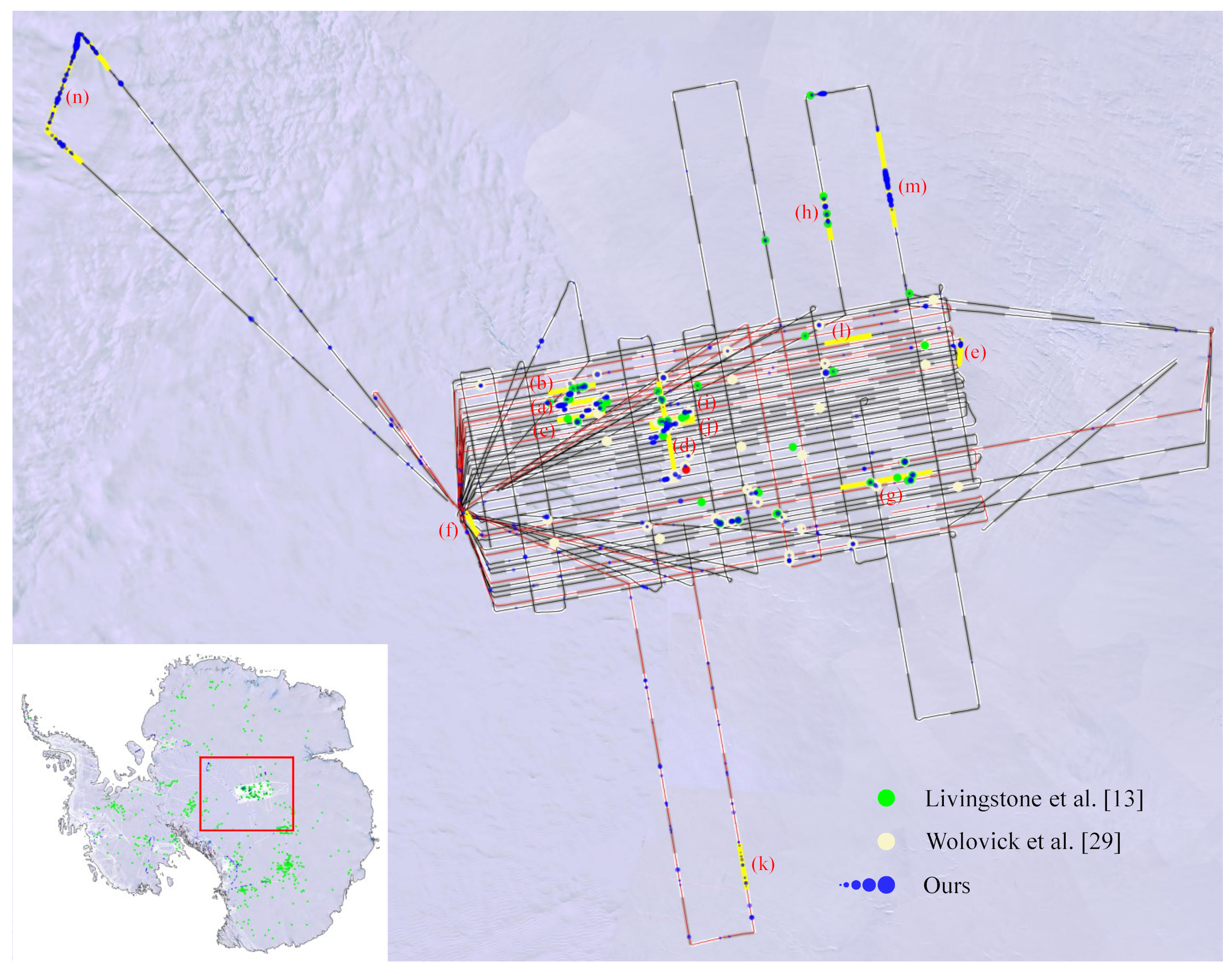
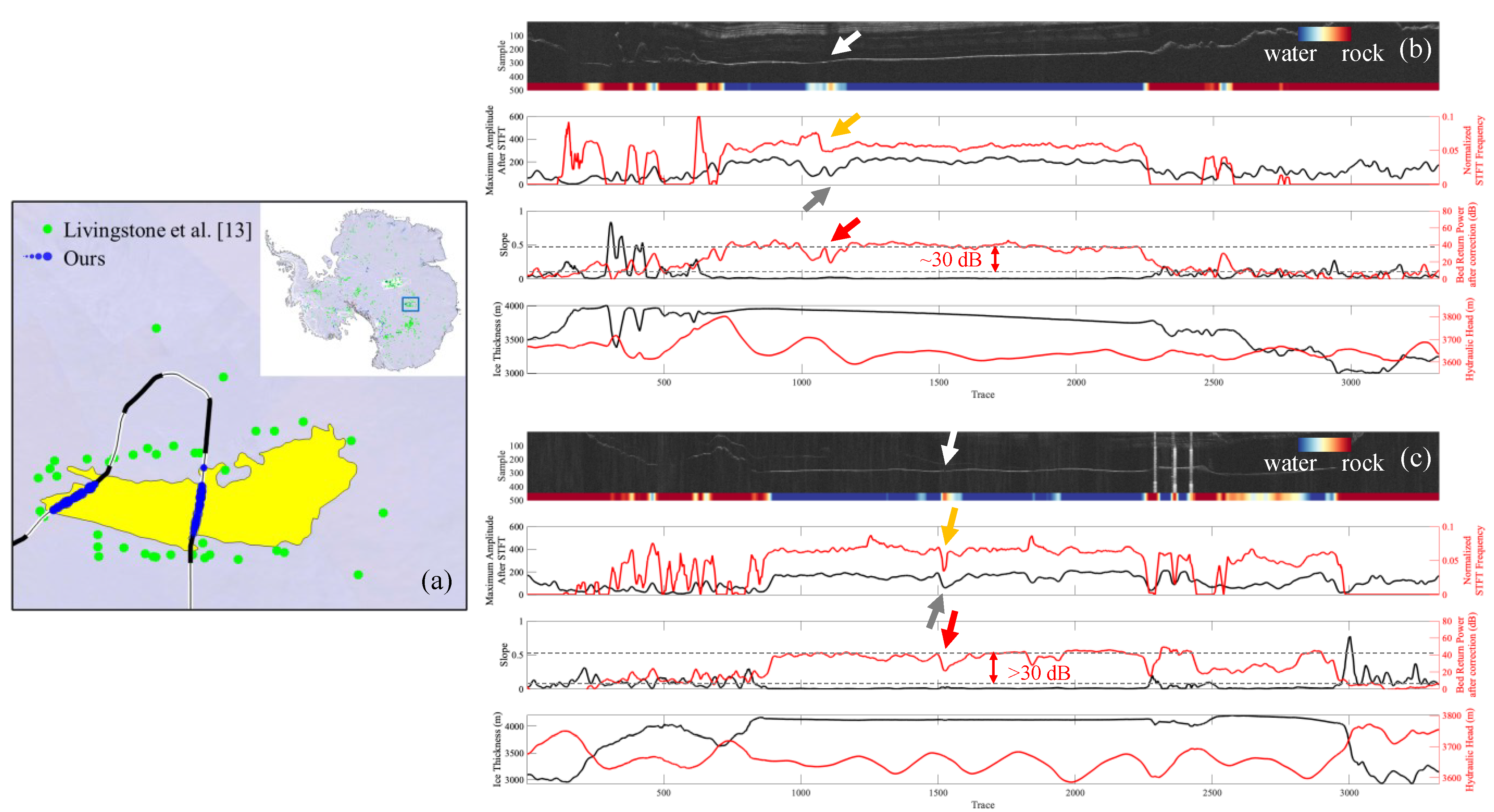
In terms of subglacial water bodies identification, the proposed method has the highest possible along-track resolution since it is implemented at the A-scope level. Compared with traditional methods, the proposed method is more effective at identifying the shape of the A-scope at the basal interface, i.e., the leading and trailing edges; hence, all the subglacial water bodies with an along-track length over 2 km in Wolovick’s inventory [29] are successfully detected by the proposed method. Moreover, five large subglacial water bodies, in Figure 7a,e,m, and more potential water body candidates, as seen in Figure 7c–e,h,j, are newly identified by the proposed method. It is worth mentioning that the threshold used in this paper is determined according to the published subglacial water bodies, which is very important for the identification of subglacial water bodies. The selection of boundaries of the subglacial water body by the proposed method tends to be more conservative and more accurate, as seen in Figure 7a, since it is implemented for each A-scope.

(2)

The proposed method has limitations in the detection of subglacial channels or small subglacial water bodies, which are too short in terms of its along-track length, due to the along-track smoothing operation [59]. As shown in Figure 8, the undetected subglacial water bodies are mostly subglacial channels with a length of less than 500 m.

(3)

The proposed method shows greater potential for the identification of basal material classification in subglacial non-water regions. The proposed method shows high accuracy for the identification of bedrock. The sedimental-like edges that gradually transit to bedrocks on both sides of the water region can also be well described by proposed method. A large sediment area is successfully identified by our method, as shown in Figure 7n, which has not been reportedly detected by traditional methods.

(4)

Similar to the traditional methods, freeze-on ice also has an impact on the identification of subglacial water bodies by the proposed method. The freeze-on ice can cause other peaks to appear next to the main peak, leading to the mis-selection of the main peak range, and thus the misinterpretation of the amplitude and frequency of the true basal interface in the radargram. This may be improved if the width of banding is reduced to exclude the freeze-on ice regions, however, this may be difficult since the freeze-on ice region is normally next to the basal interface and varies case by case.

In conclusion, this study started by evaluating the subglacial ice–water and ice–rock interfaces. Their A-scope waveforms show distinct shape contrast, which is theoretically resulted from the fact that the dielectric permittivities of bedrock and water are different. We then applied the classical STFT method to quantitatively differentiate their shapes in the frequency spectra and used the frequency signature to construct the detection formula (Equation (9)). We successfully verified the applicability of the JTFA method for the detection of subglacial water bodies using two RES datasets in the AGAP region and Lake Vostok. When qualitatively compared with Wolovick’s inventory [29], our method provides 100% accuracy in the detection of subglacial water bodies with an along-track length over 2 km, and the undetected subglacial water bodies in Figure 8 (some examples are shown in Figure 7) are mostly subglacial channels with a length of less than 500 m. On the other hand, the bedrock confirmed by our method has a very low false-positive rate. Although the identified A-scopes only takes 0.58% of the overall A-scope population in the AGAP region, the detected subglacial water bodies demonstrate excellent along-track continuity, which also show sedimental-like edges that gradually transit to bedrocks on both sides of the water region. This provides a compelling representation of how a ponded lake or water body is formed. Since the frequency analysis is conducted at the A-scope level, our method has, theoretically, the highest along-track resolution. With the frequency response, it may provide a sensible explanation of the decrease in bed return power within a suspected lake, with the hypothesis that there may exist patching isles, sedimentary shoals, or sandbank mounds that lie within a big lake or separate adjacent small lakes. As clearly demonstrated in this paper, the frequency response provided by the JTFA can be a reliable variable in the accurate identification of subglacial water bodies, which shows its potential in basal material differentiation. It may further be incorporated with many more parameters other than those used in this study (e.g., bed return power, basal roughness, hydraulic potential, ice thickness, and specular features) to serve as useful components to feed advanced deep learning algorithms for subglacial and englacial material classification.

References

1. Schlegel, N.J.; Seroussi, H.; Schodlok, M.P.; Larour, E.Y.; Boening, C.; Limonadi, D.; Watkins, M.M.; Morlighem, M.; van den Broeke, M.R. Exploration of Antarctic Ice Sheet 100-year contribution to sea level rise and associated model uncertainties using the ISSM framework. Cryosphere 2018, 12, 3511–3534. [Google Scholar] [CrossRef] [Green Version]
2. Pattyn, F.; Ritz, C.; Hanna, E.; Asay-Davis, X.; DeConto, R.; Durand, G.; Favier, L.; Fettweis, X.; Goelzer, H.; Golledge, N.R.; et al. The Greenland and Antarctic ice sheets under 1.5 °C global warming. Nat. Clim. Chang. 2018, 8, 1053–1061. [Google Scholar] [CrossRef] [Green Version]
3. Bell, R.E. The role of subglacial water in ice-sheet mass balance. Nat. Geosci. 2008, 1, 8. [Google Scholar] [CrossRef]
4. Wingham, D.J.; Siegert, M.J.; Shepherd, A.; Muir, A.S. Rapid discharge connects Antarctic subglacial lakes. Nature 2006, 440, 1033–1036. [Google Scholar] [CrossRef] [PubMed]
5. Siegert, M.J.; Ross, N.; Le Brocq, A.M. Recent advances in understanding Antarctic subglacial lakes and hydrology. Philos. Trans. A Math Phys. Eng. Sci. 2016, 374, 20140306. [Google Scholar] [CrossRef] [PubMed] [Green Version]
6. Schroeder, D.M.; Blankenship, D.D.; Young, D.A.; Quartini, E. Evidence for elevated and spatially variable geothermal flux beneath the West Antarctic Ice Sheet. Proc. Natl. Acad. Sci. USA 2014, 111, 9070–9072. [Google Scholar] [CrossRef] [PubMed] [Green Version]
7. Diez, A.; Matsuoka, K.; Jordan, T.A.; Kohler, J.; Ferraccioli, F.; Corr, H.F.; Olesen, A.V.; Forsberg, R.; Casal, T.G. Patchy Lakes and Topographic Origin for Fast Flow in the Recovery Glacier System, East Antarctica. J. Geophys. Res. Earth Surf. 2019, 124, 287–304. [Google Scholar] [CrossRef]
8. Schroeder, D.M.; Bingham, R.G.; Blankenship, D.D.; Christianson, K.; Eisen, O.; Flowers, G.E.; Karlsson, N.B.; Koutnik, M.R.; Paden, J.D.; Siegert, M.J. Five decades of radioglaciology. Ann. Glaciol. 2020, 61, 1–13. [Google Scholar] [CrossRef] [Green Version]
9. Popov, S. Ice Cover, Subglacial Landscape, and Estimation of Bottom Melting of Mac. Robertson, Princess Elizabeth, Wilhelm II, andWestern Queen Mary Lands, East Antarctica. Remote Sens. 2022, 14, 241. [Google Scholar] [CrossRef]
10. Robin, G.Q.; Swithinbank, C.; Smith, B. Radio Echo Exploration of the Antarctic Ice Sheet. IASH Publication 86; International Symposium on Antarctic Glaciological Exploration (ISAGE): Hanover, NH, USA, 1968. [Google Scholar]
11. Thakur, S.; Donini, E.; Bovolo, F.; Bruzzone, L. An Approach to the Assessment of Detectability of Subsurface Targets in Polar Ice From Satellite Radar Sounders. IEEE Trans. Geosci. Remote Sens. 2022, 60, 1–21. [Google Scholar] [CrossRef]
12. Wright, A.; Siegert, M. A fourth inventory of Antarctic subglacial lakes. Antarct. Sci. 2012, 24, 659–664. [Google Scholar] [CrossRef]
13. Livingstone, S.J.; Li, Y.; Rutishauser, A.; Sanderson, R.J.; Winter, K.; Mikucki, J.A.; Björnsson, H.; Bowling, J.S.; Chu, W.; Dow, C.F.; et al. Subglacial lakes and their changing role in a warming climate. Nat. Rev. Earth Environ. 2022, 3, 106–124. [Google Scholar] [CrossRef]
14. Siegfried, M.R.; Fricker, H.A. Illuminating Active Subglacial Lake Processes with ICESat-2 Laser Altimetry. Geophys. Res. Lett. 2021, 48, e2020GL091089. [Google Scholar] [CrossRef]
15. Neckel, N.; Franke, S.; Helm, V.; Drews, R.; Jansen, D. Evidence of cascading subglacial water flow at Jutulstraumen Glacier (Antarctica) derived from Sentinel-1 and ICESat-2 measurements. Geophys. Res. Lett. 2021, 48, e2021GL094472. [Google Scholar] [CrossRef]
16. Lindzey, L.E.; Beem, L.H.; Young, D.A.; Quartini, E.; Blankenship, D.D.; Lee, C.K.; Lee, W.S.; Lee, J.I.; Lee, J. Aerogeophysical characterization of an active subglacial lake system in the David Glacier catchment, Antarctica. Cryosphere 2020, 14, 2217–2233. [Google Scholar] [CrossRef]
17. Carter, S.P.; Blankenship, D.D.; Peters, M.E.; Young, D.A.; Holt, J.W.; Morse, D.L. Radar-based subglacial lake classification in Antarctica. Geochem. Geophys. Geosyst. 2007, 8, Q03016. [Google Scholar] [CrossRef]
18. Siegert, M.J.; Priscu, J.C.; Alekhina, I.A.; Wadham, J.L.; Lyons, W.B. Antarctic subglacial lake exploration: First results and future plans. Philos. Trans. A Math Phys. Eng. Sci. 2016, 374, 20140466. [Google Scholar] [CrossRef]
19. Yan, S.; Blankenship, D.D.; Greenbaum, J.S.; Young, D.A.; Li, L.; Rutishauser, A.; Guo, J.; Roberts, J.L.; van Ommen, T.D.; Siegert, M.J.; et al. A newly discovered subglacial lake in East Antarctica likely hosts a valuable sedimentary record of ice and climate change. Geology 2022, 50, 949–953. [Google Scholar] [CrossRef]
20. Plewes, L.A.; Hubbard, B. A review of the use of radio-echo sounding in glaciology. Prog. Phys. Geogr. 2001, 25, 34. [Google Scholar] [CrossRef]
21. Zirizzotti, A.; Cafarella, L.; Baskaradas, J.A.; Tabacco, I.E.; Urbini, S.; Mangialetti, M.; Bianchi, C. Dry–Wet Bedrock Interface Detection by Radio Echo Sounding Measurements. IEEE Trans. Geosci. Remote Sens. 2010, 48, 2343–2348. [Google Scholar] [CrossRef]
22. Popov, S.V.; Masolov, V.N. Forty-seven new subglacial lakes in the 0–110 E sector of East Antarctica. J. Glaciol. 2007, 53, 9. [Google Scholar] [CrossRef] [Green Version]
23. Siegert, M.J. Antarctic subglacial lakes. Earth-Sci. Rev. 2000, 50, 22. [Google Scholar] [CrossRef]
24. Carter, S.P.; Blankenship, D.D.; Young, D.A.; Holt, J.W. Using radar-sounding data to identify the distribution and sources of subglacial water application to Dome C, East Antarctica. J. Glaciol. 2009, 55, 16. [Google Scholar] [CrossRef] [Green Version]
25. Zirizzotti, A.; Cafarella, L.; Urbini, S. Ice and Bedrock Characteristics Underneath Dome C (Antarctica) From Radio Echo Sounding Data Analysis. IEEE Trans. Geosci. Remote Sens. 2012, 50, 37–43. [Google Scholar] [CrossRef]
26. Langley, K.; Kohler, J.; Matsuoka, K.; Sinisalo, A.; Scambos, T.; Neumann, T.; Muto, A.; Winther, J.G.; Albert, M. Recovery Lakes, East Antarctica: Radar assessment of sub-glacial water extent. Geophys. Res. Lett. 2011, 38, L05501. [Google Scholar] [CrossRef]
27. Palmer, S.J.; Dowdeswell, J.A.; Christoffersen, P.; Young, D.A.; Blankenship, D.D.; Greenbaum, J.S.; Benham, T.; Bamber, J.; Siegert, M.J. Greenland subglacial lakes detected by radar. Geophys. Res. Lett. 2013, 40, 6154–6159. [Google Scholar] [CrossRef] [Green Version]
28. Bowling, J.S.; Livingstone, S.J.; Sole, A.J.; Chu, W. Distribution and dynamics of Greenland subglacial lakes. Nat. Commun. 2019, 10, 2810. [Google Scholar] [CrossRef] [Green Version]
29. Wolovick, M.J.; Bell, R.E.; Creyts, T.T.; Frearson, N. Identification and control of subglacial water networks under Dome A, Antarctica. J. Geophys. Res. Earth Surf. 2013, 118, 1–15. [Google Scholar] [CrossRef]
30. Creyts, T.T.; Ferraccioli, F.; Bell, R.E.; Wolovick, M.; Corr, H.; Rose, K.C.; Frearson, N.; Damaske, D.; Jordan, T.; Braaten, D.; et al. Freezing of ridges and water networks preserves the Gamburtsev Subglacial Mountains for millions of years. Geophys. Res. Lett. 2014, 41, 8114–8122. [Google Scholar] [CrossRef] [Green Version]
31. Young, D.A.; Schroeder, D.M.; Blankenship, D.D.; Kempf, S.D.; Quartini, E. The distribution of basal water between Antarctic subglacial lakes from radar sounding. Philos. Trans. A Math Phys. Eng. Sci. 2016, 374, 20140297. [Google Scholar] [CrossRef]
32. Schroeder, D.M.; Blankenship, D.D.; Raney, R.K.; Grima, C. Estimating Subglacial Water Geometry Using Radar Bed Echo Specularity: Application to Thwaites Glacier, West Antarctica. IEEE Geosci. Remote Sens. Lett. 2015, 12, 443–447. [Google Scholar] [CrossRef]
33. Dowdeswell, J.A.; Siegert, J.S. The physiography of modern Antarctic subglacial lakes. Glob. Planet. Chang. 2002, 35, 221–236. [Google Scholar] [CrossRef]
34. Cooper, M.A.; Jordan, T.M.; Schroeder, D.M.; Siegert, M.J.; Williams, C.N.; Bamber, J.L. Subglacial roughness of the Greenland Ice Sheet: Relationship with contemporary ice velocity and geology. Cryosphere 2019, 13, 3093–3115. [Google Scholar] [CrossRef] [Green Version]
35. Lang, S.; Xu, B.; Cui, X.; Luo, K.; Guo, J.; Tang, X.; Cai, Y.; Sun, B.; Siegert, M.J. A self-adaptive two-parameter method for characterizing roughness of multi-scale subglacial topography. J. Glaciol. 2021, 67, 560–568. [Google Scholar] [CrossRef]
36. Oswald, G.K.A.; Gogineni, S.P. Recovery of subglacial water extent from Greenland radar survey data. J. Glaciol. 2008, 54, 94–106. [Google Scholar] [CrossRef] [Green Version]
37. Jordan, T.M.; Cooper, M.A.; Schroeder, D.M.; Williams, C.N.; Paden, J.D.; Siegert, M.J.; Bamber, J.L. Self-affine subglacial roughness: Consequences for radar scattering and basal water discrimination in northern Greenland. Cryosphere 2017, 11, 1247–1264. [Google Scholar] [CrossRef] [Green Version]
38. Ilisei, A.M.; Khodadadzadeh, M.; Ferro, A.; Bruzzone, L. An Automatic Method for Subglacial Lake Detection in Ice Sheet Radar Sounder Data. IEEE Trans. Geosci. Remote Sens. 2019, 57, 3252–3270. [Google Scholar] [CrossRef]
39. Qian, S.; Chen, D. Joint time-frequency analysis. IEEE Signal Process. Mag. 1999, 16, 52–67. [Google Scholar] [CrossRef]
40. Shreve, R.L. Movement of Water in Glaciers. J. Glaciol. 1972, 11, 205–214. [Google Scholar] [CrossRef] [Green Version]
41. Hamran, S.E.; Erlingsson, B.; Gjessing, Y.; Mo, P. Estimate of the subglacier dielectric constant of an ice shelf using a ground-penetrating step-frequency radar. IEEE Trans. Geosci. Remote Sens. 1998, 36, 8. [Google Scholar] [CrossRef]
42. Fung, A.; Chen, K. Microwave Scattering and Emission Models for Users (Artech House Remote Sensing); Artech House: Norwood, MA, USA, 2010. [Google Scholar]
43. Bell, R.E.; Ferraccioli, F.; Creyts, T.T.; Braaten, D.; Corr, H.; Das, I.; Damaske, D.; Frearson, N.; Jordan, T.; Rose, K.; et al. Widespread persistent thickening of the East Antarctic ice sheet by freezing from the base. Science 2011, 331, 1592–1595. [Google Scholar] [CrossRef] [PubMed]
44. Ferraccioli, F.; Finn, C.A.; Jordan, T.A.; Bell, R.E.; Anderson, L.M.; Damaske, D. East Antarctic rifting triggers uplift of the Gamburtsev Mountains. Nature 2011, 479, 388–392. [Google Scholar] [CrossRef] [PubMed]
45. CReSIS. 2009_Antarctica_TO_Gambit Data, Lawrence, KS, USA. Digital Media. 2021. Available online: http://data.cresis.ku.edu/ (accessed on 28 November 2022).
46. Lohoefener, A. Design and Development of a Multi-Channel Radar Depth Sounder; University of Kansas: Lawrence, KS, USA, 2006. [Google Scholar]
47. Morlighem, M.; Rignot, E.; Binder, T.; Blankenship, D.; Drews, R.; Eagles, G.; Eisen, O.; Ferraccioli, F.; Forsberg, R.; Fretwell, P.; et al. Deep glacial troughs and stabilizing ridges unveiled beneath the margins of the Antarctic ice sheet. Nat. Geosci. 2020, 13, 132–137. [Google Scholar] [CrossRef] [Green Version]
48. Griffin, D.W.; Lim, J.S. Signal estimation from modified short-time Fourier transform. IEEE Trans. Acoust. Speech Signal Process. 1984, 32, 236–243. [Google Scholar] [CrossRef]
49. Case, W.B. Wigner functions and Weyl transforms for pedestrians. Am. J. Phys. 2008, 76, 10. [Google Scholar] [CrossRef] [Green Version]
50. Wang, B.; Sun, B.; Wang, J.; Greenbaum, J.; Guo, J.; Lindzey, L.; Cui, X.; Young, D.A.; Blankenship, D.D.; Siegert, M.J. Removal of ‘strip noise’ in radio-echo sounding data using combined wavelet and 2-D DFT filtering. Ann. Glaciol. 2020, 61, 124–134. [Google Scholar] [CrossRef] [Green Version]
51. Samani, S.; Vadiati, M.; Delkash, M.; Bonakdari, H. A hybrid wavelet–machine learning model for qanat water flow prediction. Acta Geophys. 2022, 1–19. [Google Scholar] [CrossRef]
52. Xue, W.; Zhu, J.C.; Rong, X.; Huang, Y.J.; Yang, Y.; Yu, Y.Y. The analysis of ground penetrating radar signal based on generalized S transform with parameters optimization. J. Appl. Geophys. 2017, 140, 75–83. [Google Scholar] [CrossRef]
53. Wang, X.; Li, C.; Chen, W. Seismic Thin Interbeds Analysis Based on High-Order Synchrosqueezing Transform. IEEE Trans. Geosci. Remote Sens. 2022, 60, 1–11. [Google Scholar] [CrossRef]
54. He, W.; Hao, T.; Ke, H.; Zheng, W.; and Lin, K. Joint time-frequency analysis of ground penetrating radar data based on variational mode decomposition. J. Appl. Geophys. 2020, 181, 104146. [Google Scholar] [CrossRef]
55. Zhang, W.Y.; Hao, T.; Chang, Y.; Zhao, Y.H. Time-frequency analysis of enhanced GPR detection of RF tagged buried plastic pipes. NDT E Int. 2017, 92, 88–96. [Google Scholar] [CrossRef]
56. Willis, I.C.; Pope, E.L.; Leysinger Vieli, J.M.C. Drainage networks, lakes and water fluxes beneath the Antarctic ice sheet. Ann. Glaciol. 2016, 57, 96–108. [Google Scholar] [CrossRef] [Green Version]
57. Popov, S.V.; Chernoglazov, Y.B. Vostok Subglacial Lake, East Antarctica: Lake shoreline and subglacial water caves. Ice Snow 2011, 1, 12–24. (In Russian) [Google Scholar]
58. Li, J.; Paden, J.; Leuschen, C.; Rodriguez-Morales, F.; Hale, R.D.; Arnold, E.J.; Crowe, R.; Gomez-Garcia, D.; Gogineni, P. High-Altitude Radar Measurements of Ice Thickness Over the Antarctic and Greenland Ice Sheets as a Part of Operation IceBridge. IEEE Trans. Geosci. Remote Sens. 2013, 51, 742–754. [Google Scholar] [CrossRef]
59. Björnsson, H. Jökulhlaups in Iceland: Prediction, characteristics and simulation. Ann. Glaciol. 1992, 16, 95–106. [Google Scholar] [CrossRef]
Figure 1. (a) A typical B-scope radargram with one clear subglacial lake in the AGAP region. (b) The comparison of two A-scope waveforms around the ice–water (red) and ice–rock (black) interfaces.
Remotesensing 15 00363 g001
Figure 2. (a) The distribution map of the RES B-scope radargram data used in this study in the AGAP region. The red and black lines are designated as the distance between the two adjacent A-scopes, being 18 m and 30 m, respectively. (b) The flight lines overlaid the bed elevation data from BedMachine Version2 Antarctica [47].
Remotesensing 15 00363 g002
Figure 3. Flowchart of the proposed method.
Remotesensing 15 00363 g003
Figure 4. (a) B-scope radargram profile after the operation of along-track smoothing, where the red lines represent the location of 150 sampling points above and below the true basal interface. (b) B-scope radargram profile after the banding operation.
Remotesensing 15 00363 g004
Figure 5. Waveform reforming of the banded A-scope: (a) ice–water interface; (b) ice–rock interface. The blue line is the waveform after the removal of DC drift, and the red line is the waveform after the waveform reformation.
Remotesensing 15 00363 g005
Figure 6. STFT results for the identification of different basal materials. (a) The banded B-scope in which the yellow box represents a distinct subglacial lake. (b) The reformed A-scope waveform at the position of the red line in (a). (c) The STFT result of the reformed A-scope in (b), where a non-zero-frequency response is denoted by a red dot for its maximum amplitude. (d) The banded B-scope in which the yellow box represents a bedrock region. (e) the reformed A-scope waveform at the position of the black line in (d). (f) The STFT result of the reformed A-scope in (e), where a zero-frequency response is denoted by a red dot for its maximum amplitude.
Remotesensing 15 00363 g006
Figure 7. The detection and identification results of basal materials for different radar profiles in the AGAP region. (a) The B-scope of radargram frame 20081228_03_006. (b) The B-scope of radargram frame 20081225_02_024. (c) The B-scope of radargram frame 20090109_01_023. (d) The B-scope stitched together by radargram frame 20090107_03_015 and frame 20090107_03_016. (e) The B-scope of radargram frame 20081223_01_015. (f) The B-scope of radargram frame 20090102_03_001. (g) The B-scope stitched together by radargram frame 20090108_01_016 and frame 20090108_01_017. (h) The B-scope of radargram frame 20090106_05_013. (i) The B-Scope of radargram frame 20090108_03_021. (j) The B-scope of radargram frame 20081228_01_020. (k) The B-scope of radargram frame 20081226_02_017. (l) The B-scope of radargram frame 20081225_02_018. (m) The B-scope stitched together by radargram frame 20090106_05_020 and frame 20090106_05_021. (n) The B-scope stitched by radargram frame 20090107_02_014, frame 20090107_ 02_015, frame 20090107_02_016, frame 20090107_02_017, and frame 20090107_02_018. Translucent green rectangles are the boundaries of the subglacial lakes published by Livingstone et al. [13], and translucent yellow rectangles are the boundaries of the subglacial water bodies published by Wolovick et al. [29].
Remotesensing 15 00363 g007aRemotesensing 15 00363 g007b
Figure 8. The distribution of subglacial water bodies in the AGAP region. Green dots represent the inventoried subglacial lakes by Livingstone et al. [13]; yellow dots represent the inventoried subglacial water bodies by Wolovick et al. [29]; blue dots represent subglacial lakes calculated by our method, and the size of the dots represents the probability of a subglacial water body.
Remotesensing 15 00363 g008
Figure 9. (a) The comparison of results of the subglacial water bodies near Lake Vostok, whose region in yellow is redrawn according to [57]. The green dots represent the inventoried subglacial lakes by Livingstone et al. [13], and the blue dots represent subglacial lakes calculated by our method; the size of the dots represents the probability of a subglacial water body. (b,c) The detection and identification results of basal materials for different radar profiles. (b) The B-scope stitched together by radargram frame 20131127_01_039 and frame 20131127_01_040. (c) The B-scope stitched together by radargram frame 20131127_01_045 frame 20131127_01_046.
Remotesensing 15 00363 g009