Technical Note

Spatial and Temporal Sampling Properties of a Large GNSS-R Satellite Constellation

1
Department of Climate and Space Sciences and Engineering, University of Michigan, Ann Arbor, MI 48109, USA
2
Daaxa LLC, Boulder, CO 80305, USA
*
Author to whom correspondence should be addressed.
Remote Sens. 2023, 15(2), 333; https://doi.org/10.3390/rs15020333
Submission received: 21 November 2022 / Revised: 22 December 2022 / Accepted: 28 December 2022 / Published: 5 January 2023
(This article belongs to the Special Issue GNSS-R Earth Remote Sensing from SmallSats)

Abstract

:
Using large constellations of smallsats, mission designers can improve sampling density and coverage. We develop performance metrics that characterize key sampling properties for applications in numerical weather prediction and optimize orbit design parameters of the constellation with respect to those metrics. Orbits are defined by a set of Keplerian elements, and the relationship between those elements and the spatial and temporal coverage metrics are examined in order to maximize global and zonal (latitude-dependent) coverage. Additional optimization is performed by dividing a constellation into multiple orbit planes. An iterative method can be applied to this design process to compare the performance of current and previous designs. The main objective of this work is the design of optimized configurations of satellites in low Earth orbiting constellations to maximize the spatial and temporal sampling and coverage provided by its sensors. The key innovations developed are a new cost function which measures the temporal sampling properties of a satellite constellation, and the use of it together with existing cost functions for spatial sampling to design satellite constellations that optimize performance with respect to both performance metrics.

Graphical Abstract

1. Introduction

The proliferation of smallsats and the small but highly capable scientific sensors on them have ushered in a new era of Earth remote sensing from space. Technology development lifecycles have been shortened, new and improved sensors can reach space more quickly, both launch vehicle and satellite costs have been reduced dramatically, and it is now both possible and affordable to consider flying large constellations of remote sensing instruments [1]. Notably, large constellations of smallsats in low Earth orbit have the potential to significantly improve upon the spatial and temporal sampling densities provided by a single traditional large satellite [2]. The improvement in sampling density with number of spacecraft is generally intuitive—more of them spread out around the globe will tend to sample more places at the same time and to sample the same place more frequently. We consider here the optimization problems of:
  • Achieving a particular sampling density with the minimum number of satellites;
  • Maximizing the sampling density for a given number of satellites; and
  • Spreading out the samples at each location in time to better resolve diurnal variability and support the initialization of numerical weather prediction models.
The optimization is performed with respect to specific orbit parameters of the constellation, namely the number and orientation of orbit planes and the number of satellites in each plane. When quantifying the notion of sampling density, it is helpful to consider a specific type and design of remote sensing instrument. Our optimization study is performed with respect to a Global Navigation Satellite System Reflectometry (GNSS-R) sensor. These sensors are the receiver half of a bistatic radar system in which the transmitters are the existing constellation of navigation satellites, such as GPS and Galileo. Measurements of GNSS signals scattered back into space from the Earth surface contain information about a wide variety of scientifically valuable geophysical surface conditions [3,4,5,6,7]. The relevant instrument design parameters to be considered are the number of simultaneous GNSS surface reflections observed and the gain and field of view of the antenna through which the observations are made. The former design parameter affects the signal processing complexity and power requirement of the instrument, and the latter parameter affects the size and mass of the antenna. GNSS-R sensors are compatible with smallsats [8,9] and have been demonstrated to provide improved sampling density in small constellations [10], so are a natural type of measurement to consider for this study.
The satellite constellation design space being considered here is an extension of the point design used by the NASA CYGNSS mission [11]. Its constellation consists of 8 identical spacecraft spaced roughly equally around a single orbit plane at an altitude of ~525 km and an inclination angle of 35°. Each CYGNSS spacecraft carries a GNSS-R sensor capable of measuring 4 simultaneous surface reflections.

2. Discussion of Orbital Parameters, Sampling Process, and SpOCK

2.1. Constellation Design Baseline Assumptions

The achievable coverage of a constellation of remote sensing satellites is determined by both the orbit placements of the satellites within the constellation as well as the capability of the instruments carried on each satellite making the observations. Each individual satellite’s orbit is defined by the traditional six Keplarian elements: eccentricity, semi-major axis, inclination, right ascension of the ascending node (RAAN), argument of periapsis (AoP) and true anomaly [12]. For purposes of remote sensing efficacy, the key design factors of the instrument itself include antenna configuration, number of parallel observations, and minimum observation signal strength. The principle design considerations for the constellation are the total number of satellites and their orbits relative to each other. Analyzing all the possible combinations of satellites, their orbits, and instrument configurations is not impractical. Therefore, we have made several assumptions and simplifications in order to isolate and evaluate the primary parameters driving the overall measurement coverage performance. This reduces the number of constellation design variables to a manageable and useful subset. The simulations below all include the following orbit and instrument configuration constraints and assumptions:
  • All satellites are in circular orbits (eccentricy = 0, AoP not relevant), all satellites within an orbital plane are equally spaced (true anomalies fixed), all satellites in the constellation are at the same altitude (semi-major axis fixed). The number of satellites, the angular spacing of the orbit planes and the inclinations of the orbit planes are the three remaining variables considered in the constellation design;
  • The instruments on each satellite are constrained as follows: a dual antenna configuration of either (a) the NASA CYGNSS mission antennas or (b) a larger dual antenna design for the higher altitude orbit simulations. The instruments are all capable of tracking up to 16 specular reflection measurements in parallel, based on the current estimated capability of the next generation of GNSS-R instruments [13]. The signal strength required for viable land and ocean observations is based on CYGNSS retrievals vs. range corrected gain (RCG), which considers both antenna gain and path losses for individual surface measurements [14,15].
Using the above assumptions and constraints on the GNSS-R constellation configuration, the design parameters considered have been reduced to a manageable number: number of planes (incl. number of satellites per plane), inclinations of the planes, and minimum observation RCG. Each is explored individually in the sections below. The results and analysis are intended to examine the impacts of the design parameters on sampling and Earth coverage properties for possible future constellation missions.

2.2. Overview of Observation Sampling Process and Instrument Considerations

2.2.1. GNSS-R Surface Reflection Global Distribution

The global distribution of GNSS-R surface observations is the result of an asynchronous process between the orbits of the transmitting GNSS satellites (GPS, Galileo, SBAS, etc.) in Medium Earth Orbit (MEO, ~20,200 km altitude) and occasionally Geostationary orbit (~35,786 km altitude) and a constellation of Low Earth Orbit (less than 2000 km altitude) receivers below the transmitters. The GNSS-R observation point is the Earth surface location between the transmitter and receiver that results in a forward specular reflection in the direction of the receiver. An Illustration of three example GNSS-R reflection geometries is shown in Figure 1, with the transmitters above and outside the figure and a single LEO receiver capturing the parallel surface reflections. The specular reflection location point between transmitter and receiver at a single epoch can be calculated using an iterative process as described in [3]. The resulting total of GNSS-R surface reflection points is therefore driven by the pseudo-random alignment of the multiple GNSS satellites and the multiple LEO receivers that result in fortuitous surface reflection locations in the receiver antenna footprint of the GNSS-R instruments. The number of GNSS transmitters can well exceed 100 if multiple constellations are utilized (GPS, Galileo, Beidou, GLONASS) for example, while the optimal number of receivers can range into several dozen in varied orbits resulting in a dense web of overlapping surface observations. Given the large numbers of transmitters and receivers a simulation is used to generate these large data sets of surface observation points over time (nominally one day). The achieved GNSS-R observation coverage was then analyzed with respect to optimizing the spatial and temporal coverage metrics described below.

2.2.2. GNSS-R Instrument Dependencies

The GNSS-R observation distributions are highly dependent on multiple instrument configuration parameters. The number of viable science observations generated by a given instrument on a single satellite is constrained by two primary instrument capabilities: (a) the processing bandwidth of the instrument and the resulting number of available surface specular points it is capable of processing into science observations and (b) the surface area coverage of the nadir oriented GNSS-R science antennas which are required to capture the reflected signals with sufficient SNR to be usable. Other secondary spacecraft specific system requirements such as satellite down-link capability, attitude knowledge and other aspects are not analyzed here and assumed to be sufficient for the scenarios studied in this analysis.
In this analysis, the processing bandwidth of the GNSS-R instrument considers two cases: the existing on-orbit performance of the CYGNSS GNSS-R instrument which is capable of tracking 4 parallel reflections from GPS only [4], and a next Generation GNSS-R instrument (NGRx) which has shown in initial testing to be capable of tracking up to 16 parallel GNSS reflections from both GPS and Galileo [13]. It is possible that at some point in the future instruments will be capable of tracking more parallel reflections. However, we believe that 16 is a realistic estimate of the state-of-the-art GNSS-R instrument capability and grounds this analysis in existing hardware performance.
The surface coverage of the GNSS-R instrument antennas is also a key element in filtering the actual observations suitable for science applications. As expected, reflections captured in the main high gain lobes of the reflection antennas result in higher SNR observations and generally better retrievals. In this regard, we have extensive data based on the achieved performance of the CYGNSS constellation where it has been observed that ocean wind speed observations can be achieved within the mission error requirements at range corrected gain (RCG) levels of 15 and above [17]. This allows us to assess additional instrument antenna configurations with respect to this threshold and make realistic judgments as to what specular points will result in viable science observations and which specular points to omit due to low quality. In the subsequent analysis, we simulate both the actual CYGNSS antennas as well as theoretical enhanced antennas to assess the performance of different antenna gains and beam widths, as well as at alternative spacecraft altitudes to provide a more complete trade-space with respect to various spacecraft instrument configurations.

2.3. SpOCK and Its Operation

Although there are a multitude of functional mission simulation tools available for commercial and research applications, the Spacecraft Orbital Characterization Kit (SpOCK) can better predict the performances of and provide data for mission inputs that operate in a manner similar to CYGNSS. The central capability of SpOCK is a high accuracy numerical propagator of spacecraft orbits and computations of ancillary parameters [18]. The C-based programming of SpOCK allows for data variables, including CYGNSS specular points, to be easily added or subtracted in accordance with user preferences.
When creating constellations for SpOCK simulations, users can select the orbital parameters of individual satellites as well as controlling data processing tools. In text-based input files, users first describe how many satellites will be in the constellation, then provide both the individual sets of orbital parameters of each satellite and the antenna pattern used by all satellites. These inputs are read by SpOCK’s C-based simulator, and outputs are provided at a user-specified time delta in the form of multiple data files. Among these outputs is the list of constellation’s detected specular points, data that is necessary for CYGNSS’s atmospheric measurements and may not be reported by other simulation tools. Using these written output files, various performance metrics can be calculated in other programs.

2.4. Performance Metrics

The spatial coverage performance of the various constellation configurations considered is quantified by a Zonal Spatial Coverage (ZSC) metric. The Earth surface is first divided up into a 25 km grid in latitude and longitude. All grid cells in which at least one observation is made within a 24 h period are noted. Then, the percentage of grid cells sampled across all longitudes is computed in each latitude zone and that percentage is reported as a function of latitude.
We quantify the temporal coverage performance of our analyzed constellations using a Zonal Temporal Coverage (ZTC) metric. The analysis uses the same equidistant geo-spatial grid covering the entire surface of the Earth as was used for the ZSC. The simulation calculates a binary decision in every grid cell over a chosen time interval. If there was one or more observations in a given grid cell, the cell is labelled with a one (1). If no observations occurred, it would be labeled with a zero (0). The time interval we use in our analysis is six hours, with four total time intervals in a day. Therefore, the maximum ZTC coverage a location on Earth could achieve per day is 4 (i.e., at least one observation was made in each of the 4 6 h intervals in the day). This 6 h quantization of the 24 h cycle was chosen to support the input data assimilation needs of major weather prediction models with a 6-hourly reporting interval (e.g., the NOAA/NCEP Global Forecast System (GFS) and the ECMWF High Resolution 10-day Forecast (HRES). By matching our ZTC interval to the needs of the models, we address the potential value of GNSS-R observations for use by these major operational models. Naturally, analysis of other intervals with other metrics is possible. Previous studies of the sampling properties of similar satellite constellations have considered the time separation between successive samples in the same grid cell [19]. Our approach expands upon this prior work by considering the ZTC as defined above to provide a more practical and useful quantification of the temporal sampling properties as they relate to the use of the measurements by numerical weather prediction models.
For each of the constellation configurations considered below, sampling performance is derived from a population of sample times and locations generated by an orbit simulation model. The model propagates the orbital locations for each of the science observatories as well as all members of the GPS, Galileo and SBAS constellations of GNSS satellites. At each one-second time step over the course of a 24 h period, the locations of all possible surface reflections are determined for signals propagating from every GNSS satellite transmitter to every science observatory receiver via specular point reflection by the Earth surface. In addition to the time and location of each sample, the value of the receive antenna gain in the direction of the specular point reflection is also noted. This allows the signal-to-noise-ratio quality of the received signal to be determined.

3. GNSS-R Coverage Simulations

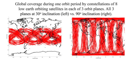
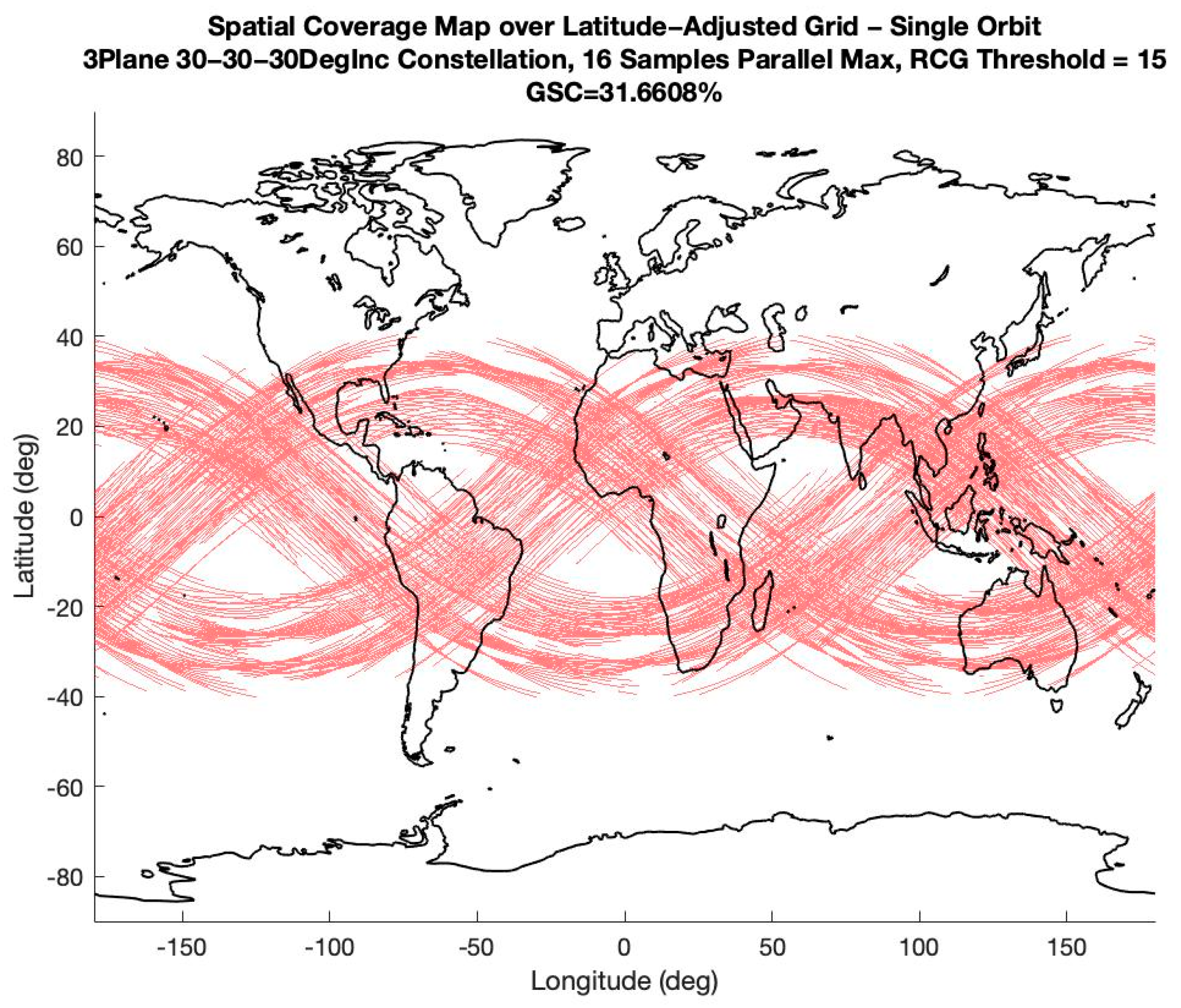
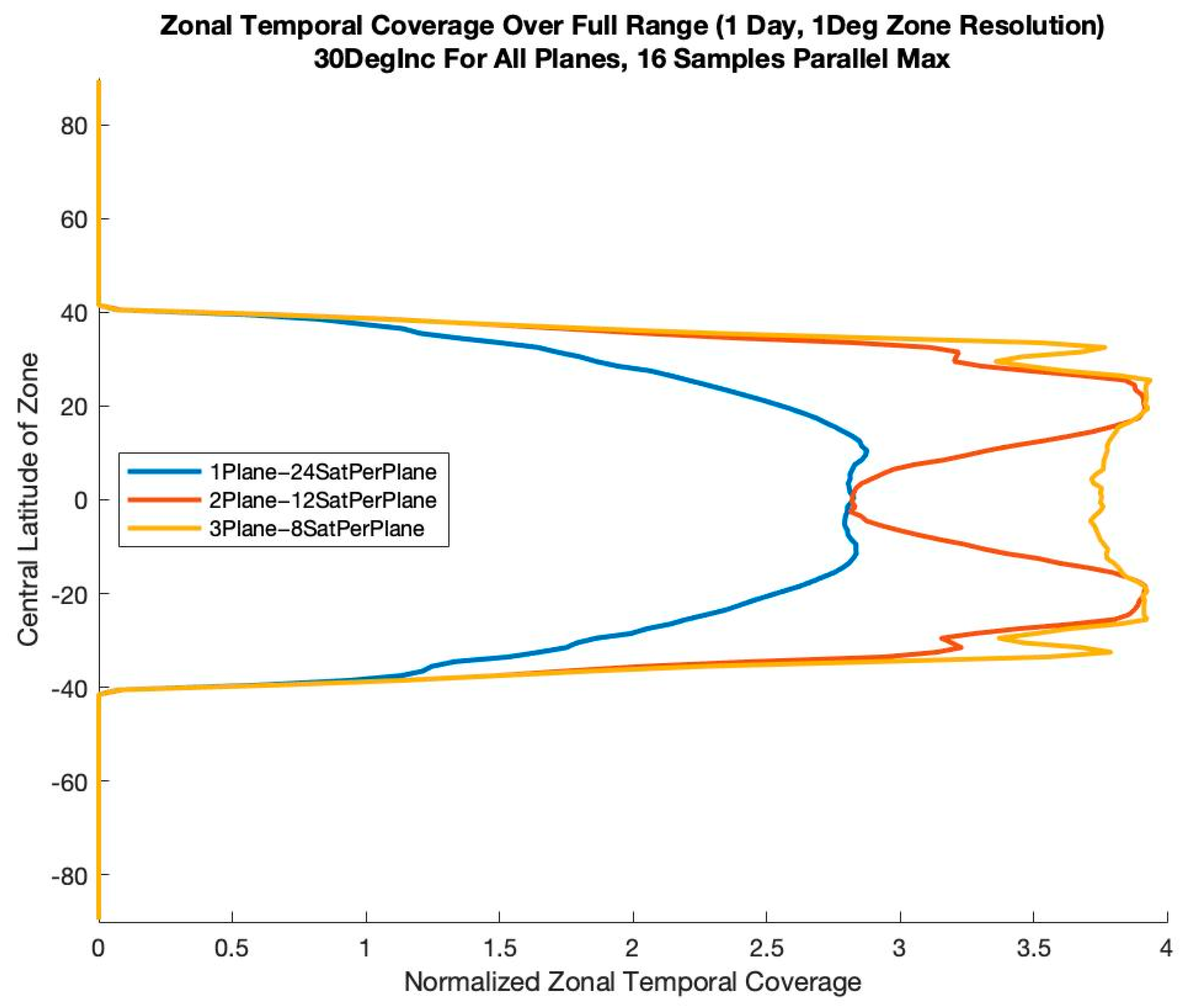
3.1. Effect of Orbit Inclincation on Constellation Coverage

One critical design feature of a constellation is the orbit inclination of its satellites. The inclination of a satellite’s orbit determines the maximum possible latitude of its surface observations and hence affects the global distribution of its spatial coverage. The inclination will also affect the frequency with which samples are made at different latitudes, which in turn determines the ZTC. These two performance considerations should both be considered in the design optimization process.
For this study, we consider design options in which one third of the total number of satellites is distributed between each of three orbit planes at distinct inclinations. We analyzed three cases, one where all three planes have an inclination of 30°, another where the three planes have inclinations of 30°, 60° and 90°, and a third where all three planes have an inclination of 90°.
The ZSC results of these simulations are illustrated in Figure 2, Figure 3 and Figure 4. Although these images depict a single orbit of these three constellations over a period of 1 h, 40 min, and 30 s, they can be extrapolated to form the full 24 h spatial coverage maps. The maximum inclination of the constellation can be seen to limit its latitudinal coverage. The coverage will not exceed the inclination by more than 10° north or south. For instance, the constellation with three planes at an inclination of 30° has non-zero ZSC at latitudes slightly lower than 40° north and south. However, after extrapolating the three orbit maps, this truncated coverage will contrast with the almost 100% ZSC performance demonstrated by the 30°-60°-90° and 90°-90°-90° inclination constellations. In these situations where the maximum inclination of the constellation is set to 90°, the constellations are capable of taking measurements over the entire Earth.
The ZTC results of these simulations are illustrated in Figure 5. When all constellation planes operate at the same inclination, the ZTC peaks around those latitudes. However, when the plane inclinations are more evenly spaced between latitude levels, as shown by the 30°-60°-90° constellations, we get more well-distributed sampling across the Earth at the cost of smaller coverage peaks.

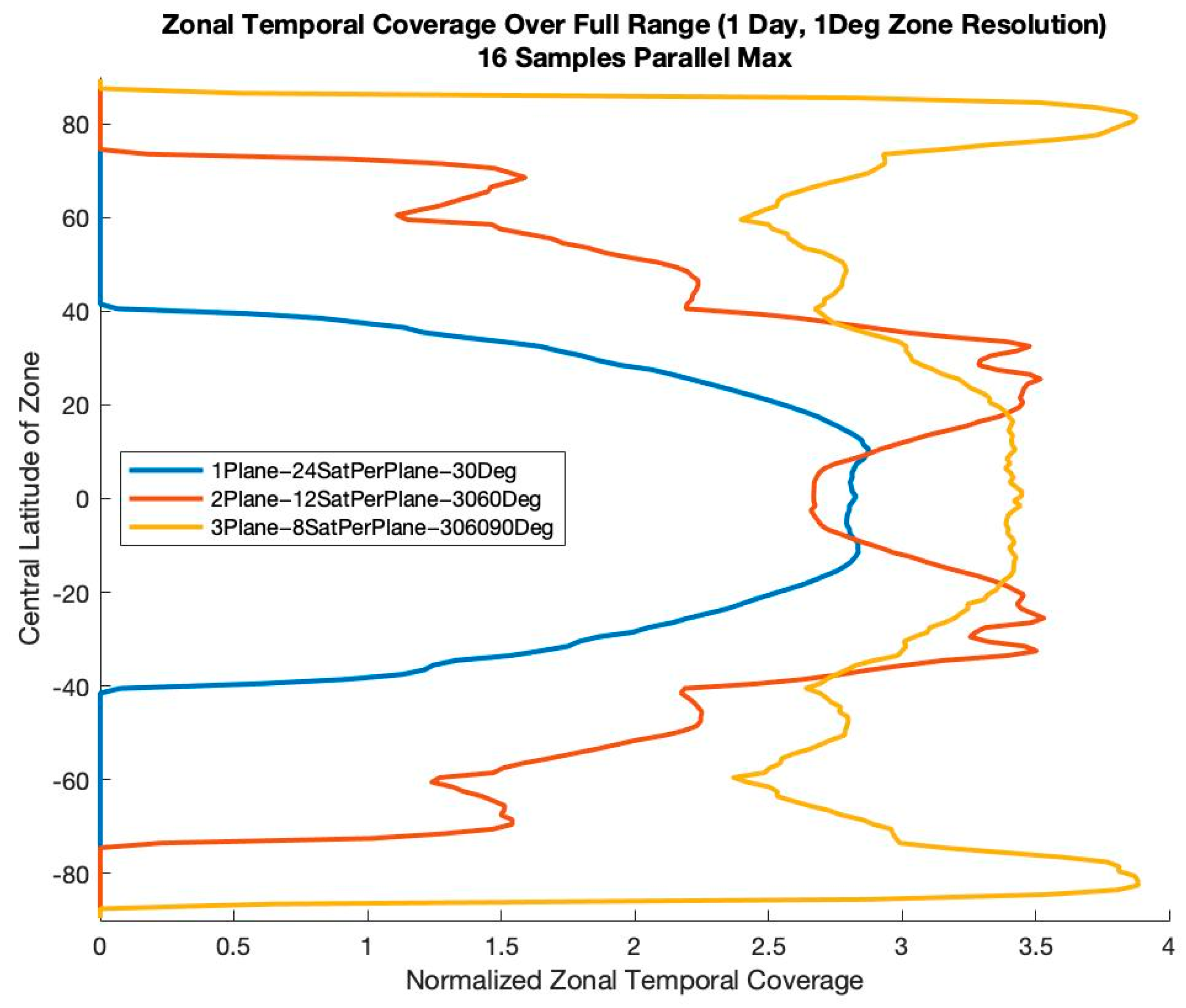
3.2. Effect of Orbit Planes on Constellation Coverage

The second critical design feature of a constellation is how its satellites are distributed between orbit planes. In this series of design options, an orbit plane is defined as a group of satellites orbiting with the same ascending node longitude. With that definition in mind, we find that when a singular plane satellite constellation is divided into a constellation with multiple planes, its ZTC increases. However, when only looking at certain latitude zones on the globe, this trend may not be uniform.
To better understand how the temporal coverage depends on the distribution of planes, two experiments were conducted where the total number of satellites and satellite inclination were held constant. These experiments first simulate the performance of a single plane of 24 evenly distributed satellites all orbiting at the same inclination. Then, the simulation is repeated for a second constellation in which the plane is split into two planes of twelve evenly distributed satellites separated by 180° longitude. Finally, a third constellation is considered in which the satellites are further split into three planes of eight evenly distributed satellites separated by 120° longitude. These results are presented in Figure 6, where the orbit inclination is set to 30°.
In this scenario, the ZTC in the zone near the orbit peaks grows when the original constellation is divided into more planes. There is also a ZTC increase at latitudes lower than the peaks when the constellation is redistributed from one plane to three planes. However, when observing the two-plane constellation, the ZTC measurements at latitudes near the equator can remain near stagnant.
Using this understanding of orbit planes and inclinations, designers can better tune their constellation orientations so that both spatial and temporal coverage metrics are optimized. For this experiment, we consider a constant number of satellites all at the same inclination and in the same plane. In this case, a 24-satellite constellation at 30° inclination is selected. The performance of this constellation is seen in the blue curve of Figure 7. Note that coverage is lacking near 60°. To improve it, we divide the plane into a constellation of two 12-satellite planes, one of which orbits at 30° and the other at 60°, resulting in the red curves in Figure 7. As these curves demonstrate, adding this second plane at a higher inclination has the desired effect of increasing coverage above 30°. Furthermore, if coverage at even higher latitudes was desired, the constellation could be divided into a third plane with an inclination of 90°. This third plane will also eliminate the coverage drop near the equator present in constellations with two planes.

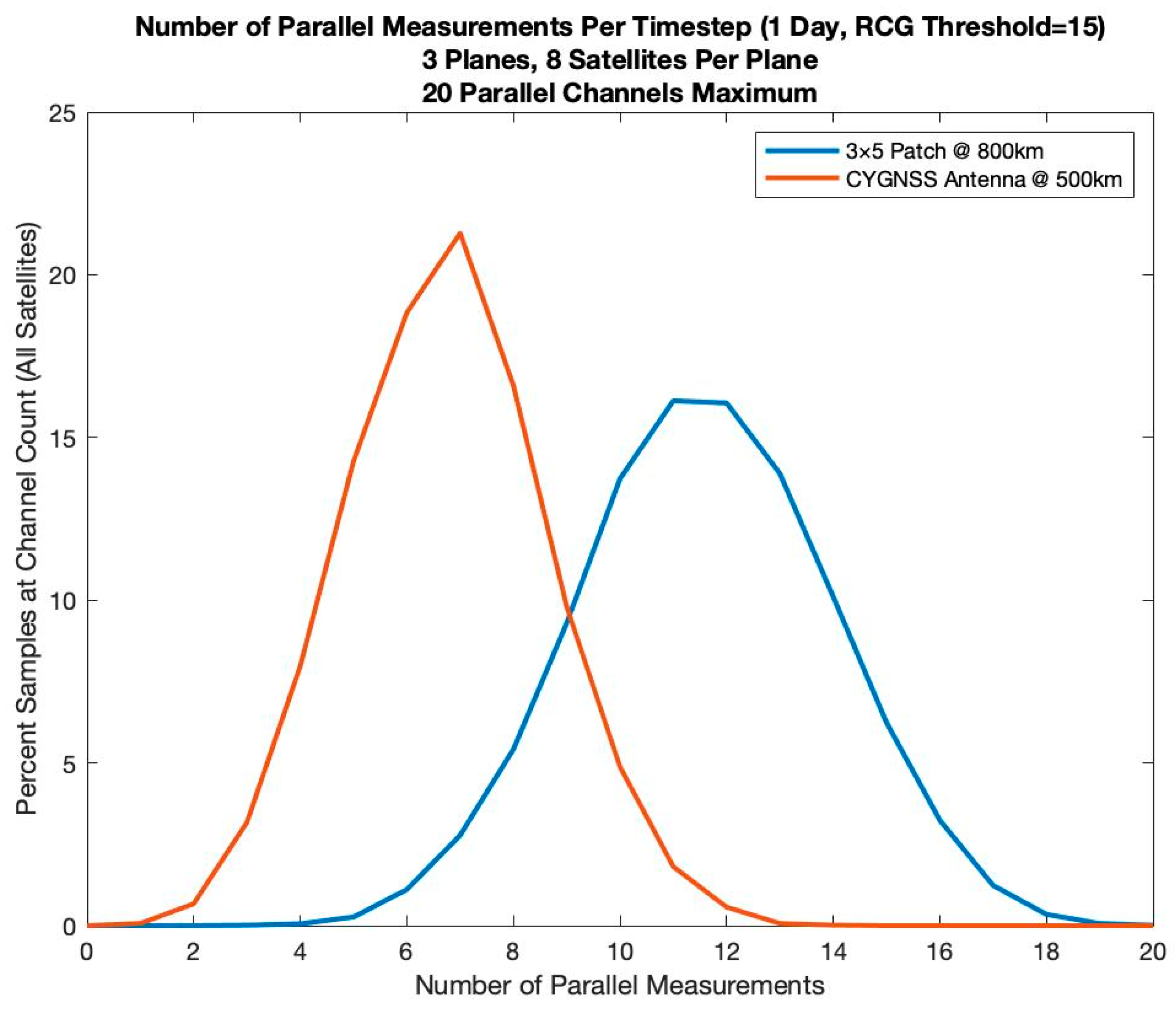
3.3. Effect of Measurement RCG on Constellation Coverage

A third critical design feature of a constellation is the antenna gain of its measurements. The impact of antenna gain on science measurement quality is characterized by the Range Corrected Gain (RCG). A higher RCG represents higher signal-to-noise ratio data and higher quality estimates of geophysical quantities derived from them, such as ocean surface wind speed [17]. Two ways are considered to control the RCG values, changing the design of the receiving antenna assumed on each of the satellites and raising the RCG threshold required for data usage.
The antenna used by a GNSS-R sensor is typically designed to accommodate a particular orbit altitude. A higher altitude will increase the propagation distance and decrease the received signal strength. This decrease can be mitigated by increasing the antenna gain. Alternatively, a decrease in altitude will restrict the field of view of an antenna pattern projected onto the Earth surface. This restriction can be mitigated by widening the antenna pattern. Fortuitously, a wider antenna pattern tends to have a lower antenna gain, so these two considerations can be accommodated jointly by the same adjustment in antenna design as a function of orbit altitude. Two orbit altitudes and corresponding antenna designs are considered here. The first assumes a similar configuration as is used by the CYGNSS constellation—namely a 500 km altitude and a 2 × 3 element phased array antenna. Although CYGNSS operates at an altitude of 525 km, the results at 500 km provides nearly identical performance. The second option is an 800 km orbit and a 3 × 5 element phased array antenna. The advantage of the higher orbit altitude is wider field of view of the antenna, which allows for more available specular point reflections to be sampled. This is demonstrated in the curves of Figure 8. When we compare the RCG values of samples collected from the CYGNSS configuration and the 3 × 5 antenna at 800 km altitude, we can see that the CYGNSS antenna will retrieve significantly fewer parallel measurements for the same RCG threshold as the 3 × 5 patch antenna, demonstrating the advantage of a higher altitude orbit.
It is important to consider where the minimum RCG threshold is set. A threshold of 15 has been found to be sufficient for providing high-quality science data to most applications. The implications of this threshold on the number of usable samples are illustrated in Figure 9. The figure considers the fraction of all samples retained given different lower-bound RCG thresholds. The reference baseline is usage of all samples (i.e., no threshold). The results show that all three constellations will have 50% of collected data fall below threshold when it is set to RCG > 15.

4. Examples

4.1. Application of Design Methodology

By qualifying these three design spaces, they can now be applied towards optimizing a constellation design. One potential optimization task could be to maximize ZTC at all latitudes while maintaining ZSC as close to 100% at those same latitudes.
For this scenario, it can be assumed that 24 satellites are available for use similarly to the examples discussed previously in this report. By doing so, this constellation will have more than enough satellites to guarantee a near 100% ZSC over the course of a 24 h test while allowing for greater manipulability of its ZTC. With 24 satellites provided, a constellation designer would then need to decide how to spatially organize these elements. As described above in Section 3.2, the most practical pattern organization would be to divide the 24 satellites into 3 evenly distributed planes of 8 satellites. The result of doing so while holding other variables constant is further illustrated in Figure 6.
Once the satellites are placed into orbit planes, it is up to the constellation designer to set each plane’s orbit inclination. To maintain near 100% GSC while having an evenly distributed ZTC, it would make sense to start with a configuration with planes inclined at 30°, 60°, and 90°. Since there is a plane inclined at 90°, not only is a GSC near 100% as described in Section 3.1, but also a ZTC distribution as illustrated in Figure 5 will be achieved. However, when observing this ZTC distribution over latitude, it can be noted that both the ZTC drops significantly near 60° and the ZTC at other latitudes below 80° are significantly below the maximum coverage value of 4. This behavior can be observed by analyzing the coverage metrics across larger zones, defined as equatorial, mid-latitude, and polar. More specifically, the equatorial zone is bounded by the latitudes 30°S and 30°N, the mid-latitude zone is defined by the two sets of boundaries, 30–60° north and south, and the polar zone is defined by the two sets of boundaries, 60–90° north and south. As illustrated in Table 1, the mid-latitude and polar ZTC measurements for the 30°-60°-90° constellation are significantly lower than the equatorial ZTC. When considering this information along with the ZTC plot in Figure 5, the mid-latitude and polar ZTC drops can be attributed to the smaller quantity of satellites in polar orbits and the placement of the mid-latitude plane at 60° inclination. In order to overcome the lack of uniformity and raise the overall ZTC, it is necessary to adjust each plane’s inclination. An alternative approach is to design fitness functions that score constellations based on these coupled global performance metrics [19].
There are two possible approaches for correcting the ZTC drop near 60°. First, a designer can either raise the inclination of first plane, which was initially placed at 30°, or lower the inclination of the third plane, which was initially placed at 90°. By adjusting these inclinations, additional coverage can be shifted towards the latitude where ZTC is lacking. However, shifting too much may cause new significant drops to form. Second, a designer can raise or lower the inclination of the second plane, which was initially placed at 60°. Although this approach may not eliminate the ZTC drop, it will reposition it to a latitude where it may become more simple to perform the first method.
Starting from the baseline of a 3-Plane 30°-60°-90° constellation, the progression of this logic and the corresponding changes in GSC, ZSC, GTC, and ZTC are illustrated by the results provided in Table 1. After a few iterations, we find a significant improvement from the original baseline in the 3-Plane 50°-75°-80° constellation. In each step of the process, GSC always remains close to a complete 100%, but most progressions showed growth in the GTC of each prototype constellation. By incrementally raising the first plane inclination, we can slowly increase the GTC. However, once we reach a point where the first two inclinations are starting to get closer, we find that raising the second plane would create a more significant increase in this metric. This is evident by the GTC change between the 45°-60°-90° and the 45°-65°-90° constellations. Additionally, the increase in the inclination of the first plane from 45° to 50° allows for one more small rise in GTC without moving the first plane too close to the second plane while allowing for significant equator coverage. Finally, we can take advantage of the 10° reach from the set inclination to lower the third plane down from 90° to 80° while both improving ZTC at inclinations lower than 80° and maintaining the ZTC between 80° and 90°.
When comparing this 50°-75°-80° constellation to others with no separation in plane inclinations, such as the 30°-30°-30° or 90°-90°-90°, the differences in GTC and ZTC are prominent. Since the 30°-30°-30° constellation’s max inclination is equatorial, its mid-latitude ZTC, polar ZTC, and GTC are all much smaller than other constellations considered, making it less than ideal for a globally effective design. On the other hand, the 90°-90°-90° constellation has a relatively large GTC, but its equatorial ZTC is much smaller than other designs considered. Although the 50°-75°-80° constellation does not have the largest ZTC of these three constellations in any of the regions, its zonal and global metrics are still relatively good. Considering the goal of this design study is to maximize ZTC at all latitudes, the 50°-75°-80° constellation is a good design candidate, for its zonal metrics are large at all latitudes and are further characterized by a large GTC.

4.2. Sampling of a Landfalling Hurricane

To illustrate the scientific implications of the sampling properties of an optimized constellation of GNSS-R satellites, a specific example is considered. Hurricane Ida made landfall along the U.S. Louisiana coast on 29 August 2021 at 1655 UTC. The measurements that would have been made on that day by two different GNSS-R constellations have been simulated and overlaid with GOES imagery of the storm. One constellation consists of 8 satellites arranged in a common orbit plane at an inclination of 30°, similar to the CYGNSS configuration. The other constellation consists of 8 satellites in each of 3 orbit planes with RAANs of 0°, 120° and 240° and a common 30° inclination. The global coverage with this configuration was shown in Figure 2. All spacecraft in both constellations are assumed to be capable of 16 simultaneous specular reflection measurements. Results of the simulation are shown in Figure 10. In the figure, four 6-hourly intervals of time are considered, consistent with the initialization time increment between operational numerical hurricane forecasts. All samples made during each 6 h interval are shown, together with the GOES image of the storm taken at the center of the four time intervals, namely at 0600, 1200, 1800 and 2400 UTC on 29 August.
In Figure 10, the right column corresponds to measurements made by the 24 spacecraft distributed over 3 orbit planes. In each 6 h interval, the storm is well sampled both in its inner core region and across the surrounding wind field in all four principle quadrants. Inner core measurements support the determination of maximum sustained winds and hurricane intensity, while coverage of the wider wind field supports the determination of storm size and duration during landfall. The left-hand column in Figure 10 corresponds to measurements made by the 8 spacecraft constellation. The storm is quite well sampled throughout the inner core and surrounding wind field during only one of the four 6 h intervals (1500–2100 UTC). In two of the other intervals, samples are made over only two of the four principle quadrants of the storm, with little of the inner core sampled in either case. The fourth 6 h interval has no samples whatsoever of the storm.

5. Conclusions

Large constellations of smallsats in low Earth orbit can provide spatial and temporal coverages with greater sampling density relative to constellations with fewer large satellites. This increase in coverage is primarily characterized by three factors and quantified by zonal and global measurements. The selection of satellite inclinations allows designers to choose which latitude zones are receiving more coverage while also optimizing global visibility. Meanwhile, dividing a constellation into multiple orbit planes allows designers to further improve global and zonal temporal coverage figures. Additionally, the quality and quantity of the permissible sensed data can be controlled by selecting an appropriate RCG threshold in accordance with constellation’s onboard GNSS-R instruments. Ultimately, these parameters allow for designers to iteratively evaluate constellation prototypes and maximize spatial and temporal coverage both globally and in regions of interest.
When designing a constellation, each mission will have its own set of objectives where it wants to maximize its coverage. However, the most generic definition of a successful constellation design would be maximizing global coverage metrics while keeping zonal coverage metrics evenly distributed. Through an iterative process of adjusting the satellite inclinations of 3-plane constellations, it has been found that a constellation with planes of 8 satellites orbiting at inclinations of 50°, 75° and 80° meet these design goals. Although it may be possible to adjust the definition of success to meet specific mission requirements, this constellation has been found to provide quite good overall coverage both globally and zonally.

Author Contributions

Conceptualization, C.R. and S.G.; methodology, J.W., C.R. and S.G.; software, J.W.; validation, J.W., C.R. and S.G.; formal analysis, J.W., C.R. and S.G.; investigation, J.W., C.R. and S.G.; resources, C.R.; data curation, C.R.; writing—original draft preparation, J.W., C.R. and S.G.; writing—review and editing, J.W., C.R. and S.G.; visualization, J.W.; supervision, C.R. and S.G.; project administration, C.R.; funding acquisition, C.R. All authors have read and agreed to the published version of the manuscript.

Funding

This research and the APC were funded by NASA contract number 80LARC21DA003.

Data Availability Statement

No new data were created in performance of the work presented here.

Conflicts of Interest

The authors declare no conflict of interest.

References

  1. NASEM. Leveraging Commercial Space for Earth and Ocean Remote Sensing; The National Academies Press: Washington, DC, USA, 2022. [Google Scholar] [CrossRef]
  2. Bussy-Virat, C.D.; Ruf, C.S.; Ridley, A.J. Relationship Between Temporal and Spatial Resolution for a Constellation of GNSS-R Satellites. IEEE J. Sel. Top. Appl. Earth Obs. Remote Sens. 2018, 12, 16–25. [Google Scholar] [CrossRef]
  3. Gleason, S.; Gebre-Egziabher, D. GNSS Applications and Methods, 1st ed.; Artech House: Norwood, MA, USA, 2009; p. 508. [Google Scholar]
  4. Katzberg, S.J.; Dunion, J.; Ganoe, G.G. The use of reflected GPS signals to retrieve ocean surface wind speeds in tropical cyclones. Radio Sci. 2013, 48, 371–387. [Google Scholar] [CrossRef]
  5. Unwin, M.; Jales, P.; Tye, J.; Gommenginger, C.; Foti, G.; Rosello, J. Spaceborne GNSS-Reflectometry on TechDemoSat-1: Early Mission Operations and Exploitation. IEEE J. Sel. Top. Appl. Earth Obs. Remote Sens. 2016, 9, 4525–4539. [Google Scholar] [CrossRef]
  6. Carreno-Luengo, H.; Lowe, S.; Zuffada, C.; Esterhuizen, S.; Oveisgharan, S. Spaceborne GNSS-R from the SMAP Mission: First Assessment of Polarimetric Scatterometry over Land and Cryosphere. Remote Sens. 2017, 9, 362. [Google Scholar] [CrossRef] [Green Version]
  7. Pierdicca, N.; Comite, D.; Camps, A.; Carreno-Luengo, H.; Cenci, L.; Clarizia, M.P.; Costantini, F.; Dente, L.; Guerriero, L.; Mollfulleda, A.; et al. The Potential of Spaceborne GNSS Reflectometry for Soil Moisture, Biomass, and Freeze–Thaw Monitoring: Summary of a European Space Agency-funded study. IEEE Geosci. Remote Sens. Mag. 2021, 10, 8–38. [Google Scholar] [CrossRef]
  8. Ruf, C.S.; Atlas, R.; Chang, P.S.; Clarizia, M.P.; Garrison, J.L.; Gleason, S.; Katzberg, S.J.; Jelenak, Z.; Johnson, J.T.; Majumdar, S.J.; et al. New Ocean Winds Satellite Mission to Probe Hurricanes and Tropical Convection. Bull. Am. Meteorol. Soc. 2016, 97, 385–395. [Google Scholar] [CrossRef]
  9. Jales, P.; Esterhuizen, S.; Masters, D.; Nguyen, V.; Nogués-Correig, O.; Yuasa, T.; Cartwright, J. The new Spire GNSS-R satellite missions and products. In Proceedings of the Image and Signal Processing for Remote Sensing XXVI 2020, Online, 20 September 2020; Volume 11533, p. 1153316. [Google Scholar] [CrossRef]
  10. Ruf, C.; Asharaf, S.; Balasubramaniam, R.; Gleason, S.; Lang, T.; McKague, D.; Twigg, D.; Waliser, D. In-Orbit Performance of the Constellation of CYGNSS Hurricane Satellites. Bull. Am. Meteorol. Soc. 2019, 100, 2009–2023. [Google Scholar] [CrossRef]
  11. Rose, R.; Ruf, C.; Rose, D.; Brummitt, M.; Ridley, A. The CYGNSS flight segment; A major NASA science mission enabled by micro-satellite technology. In Proceedings of the 2013 IEEE Aerospace Conference, Big Sky, MT, USA, 2–9 March 2013; pp. 1–13. [Google Scholar] [CrossRef]
  12. Roddy, D. Satellite Communications, 4th ed.; McGraw-Hill: New York, NY, USA, 2006; pp. 32–36. [Google Scholar]
  13. Ruf, C.; Backhus, R.; Butler, T.; Chen, C.-C.; Gleason, S.; Loria, E.; McKague, D.; Miller, R.; O’Brien, A.; van Nieuwstadt, L. Next Generation GNSS-R Instrument. In Proceedings of the IGARSS 2020-2020 IEEE International Geoscience and Remote Sensing Symposium, Waikoloa, HI, USA, 26 September–2 October 2020; pp. 3353–3356. [Google Scholar] [CrossRef]
  14. Gleason, S.; Ruf, C.S.; O’Brien, A.J.; McKague, D.S. The CYGNSS Level 1 Calibration Algorithm and Error Analysis Based on On-Orbit Measurements. IEEE J. Sel. Top. Appl. Earth Obs. Remote Sens. 2018, 12, 37–49. [Google Scholar] [CrossRef]
  15. Ruf, C.; Chang, P.; Clarizia, M.P.; Gleason, S.; Jelenak, Z.; Murray, J.; Morris, M.; Musko, S.; Posselt, D.; Provost, D.; et al. CYGNSS Handbook; Michigan Pub.: Ann Arbor, MI, USA, 2016; p. 154. ISBN 978-1-60785-380-0. [Google Scholar]
  16. Zavorotny, V.U.; Gleason, S.; Cardellach, E.; Camps, A. Tutorial on Remote Sensing Using GNSS Bistatic Radar of Opportunity. IEEE Geosci. Remote Sens. Mag. 2015, 2, 8–45. [Google Scholar] [CrossRef] [Green Version]
  17. Ruf, C.; Gleason, S.; McKague, D.S. Assessment of CYGNSS Wind Speed Retrieval Uncertainty. IEEE J. Sel. Topics Appl. Earth Obs. Remote Sens. 2018, 12, 87–97. [Google Scholar] [CrossRef]
  18. Bussy-Virat, C.; Getchius, J.; Ridley, A. The Spacecraft Orbital Characterization Kit and its Applications to the CYGNSS Mission. In Proceedings of the 2018 Space Flight Mechanics Meeting, Kissimmee, FL, USA, 8–12 January 2018. [Google Scholar] [CrossRef]
  19. Tan, C.; Xu, Y.; Luo, R.; Li, Y.; Yuan, C. Low Earth orbit constellation design using a multi-objective genetic algorithm for GNSS reflectometry missions. Adv. Space Res. 2022, in press. [Google Scholar] [CrossRef]
Figure 1. General illustration of three GNSS-R reflection specular points captures by a single LEO receiver. Reprinted with permission from ref. [16], Copyright: 2014, IEEE.
Remotesensing 15 00333 g001
Figure 2. Single-Orbit Spatial Coverage for 3-Plane 30°-30°-30° constellation at 800 km, 16 parallel measurements per sampling, and operating with an RCG Threshold of 15. The lower maximum inclination limits spatial coverage to below 40° latitude.
Remotesensing 15 00333 g002
Figure 3. Single-Orbit Spatial Coverage for 3-Plane 30°-60°-90° constellation at 800 km, 16 parallel measurements per sampling, and operating with an RCG Threshold of 15. The inclination distribution provides greater coverage at the various orbit peaks, allowing for a greater GSC than the 30°-30°-30° constellation.
Remotesensing 15 00333 g003
Figure 4. Single-Orbit Spatial Coverage for 3-Plane 90°-90°-90° constellation at 800 km, 16 parallel measurements per sampling, and operating with an RCG Threshold of 15. The 90° maximum plane inclination allows the constellation to achieve near 100% GSC after 24 h.
Remotesensing 15 00333 g004
Figure 5. 24 h Temporal Coverage measurements at different latitudes for 3-Plane constellations at 800 km, 16 parallel measurements per sampling, and operating with an RCG Threshold of 15. Raising the inclination of individual planes or the entire constellation can alter which latitudes are visited most often.
Remotesensing 15 00333 g005
Figure 6. 24 h Temporal Coverage measurements at different latitudes for 24-satellite constellations at 800 km, 30° inclination, 16 parallel measurements per sampling, and operating with an RCG Threshold of 15. Increasing the number of constellation planes while keeping the total number of satellites constant will increase the constellation’s Zonal and Global Temporal Coverage.
Remotesensing 15 00333 g006
Figure 7. 24 h Temporal Coverage measurements at different latitudes for 24-satellite constellations at 800 km, 16 parallel measurements per sampling, and operating with an RCG Threshold of 15. As the initial 30° inclination plane of 24 satellites is divided in smaller planes with raised inclinations allows the constellation’s Zonal and Global Temporal Coverage to be shaped and increased.
Remotesensing 15 00333 g007
Figure 8. Parallel Measurement Comparison between antenna patterns at their corresponding altitudes over 24 h using a 3-Plane constellation with each plane at 30°, 60°, and 90° inclination, 20 Parallel Measurements Maximum per sampling, and an RCG Threshold of 15.
Remotesensing 15 00333 g008
Figure 9. RCG Thresholding Comparison for 3-Plane constellations at 800 km, 16 parallel measurements per sampling, and with 8 satellites per plane. For all listed constellations, the fraction of measurements below threshold converges around RCG Value of 15.
Remotesensing 15 00333 g009
Figure 10. Simulated measurements by two GNSS-R constellations of Hurricane Ida during landfall on 29 August 2021. The left column corresponds to an 8-satellite constellation and the right to one with 24 satellites, all at 30° inclination. Rows correspond to 6 h time intervals centered on 0600, 1200, 1800 and 2400 UTC. GNSS-R tracks are overlaid on GOES-16 Band 8 (6.17 μm) images at the center times. Landfall occurred at 1655 UTC.
Remotesensing 15 00333 g010
Table 1. Constellation Optimization through the Proposed Iterative Method. The constellations all feature 3 evenly distributed orbit planes of 8 evenly spaced satellites per plane at an altitude of 800 km. The coverage metrics described above were evaluated with the 3 × 5 element phased array antenna and a RCG minimum threshold of 15. By making these discrete adjustments in the inclinations of individual planes, we can keep the GSC near 100% while incrementally improving the GTC.
Constellation (deg-deg-deg)Global Spatial Coverage (%)Global Temporal CoverageZSC
(eq)
ZSC
(mid)
ZSC
(Polar)
ZTC
(eq)
ZTC
(mid)
ZTC
(Polar)
30-30-3062.9872.25499.99435.50503.7880.9830
90-90-9099.3373.15199.21499.79698.5402.8883.2733.795
30-60-9099.6883.06999.94999.75698.2383.2832.7162.881
35-60-9099.6773.05399.94399.84098.2383.2782.8092.881
40-60-9099.6793.07999.91299.88798.2383.2522.9172.881
45-60-9099.6763.10299.88699.91698.2383.2143.0322.881
45-65-9099.7263.17499.90099.97598.4003.2613.1003.174
45-70-9099.7213.18099.88699.96298.4483.2373.1043.175
45-75-9099.8143.18199.87099.95199.2273.2073.0963.313
50-75-9099.8003.19999.82999.96999.2273.1713.1943.319
50-75-8099.9123.25299.84699.97199.9943.1863.2593.478
Disclaimer/Publisher’s Note: The statements, opinions and data contained in all publications are solely those of the individual author(s) and contributor(s) and not of MDPI and/or the editor(s). MDPI and/or the editor(s) disclaim responsibility for any injury to people or property resulting from any ideas, methods, instructions or products referred to in the content.

