
Dynamic Characteristics of Vegetation Change Based on Reconstructed Heterogenous NDVI in Seismic Regions

 ,
,  , ,
, ,  , ,
, ,
Abstract
1. Introduction
2. Data and Methods
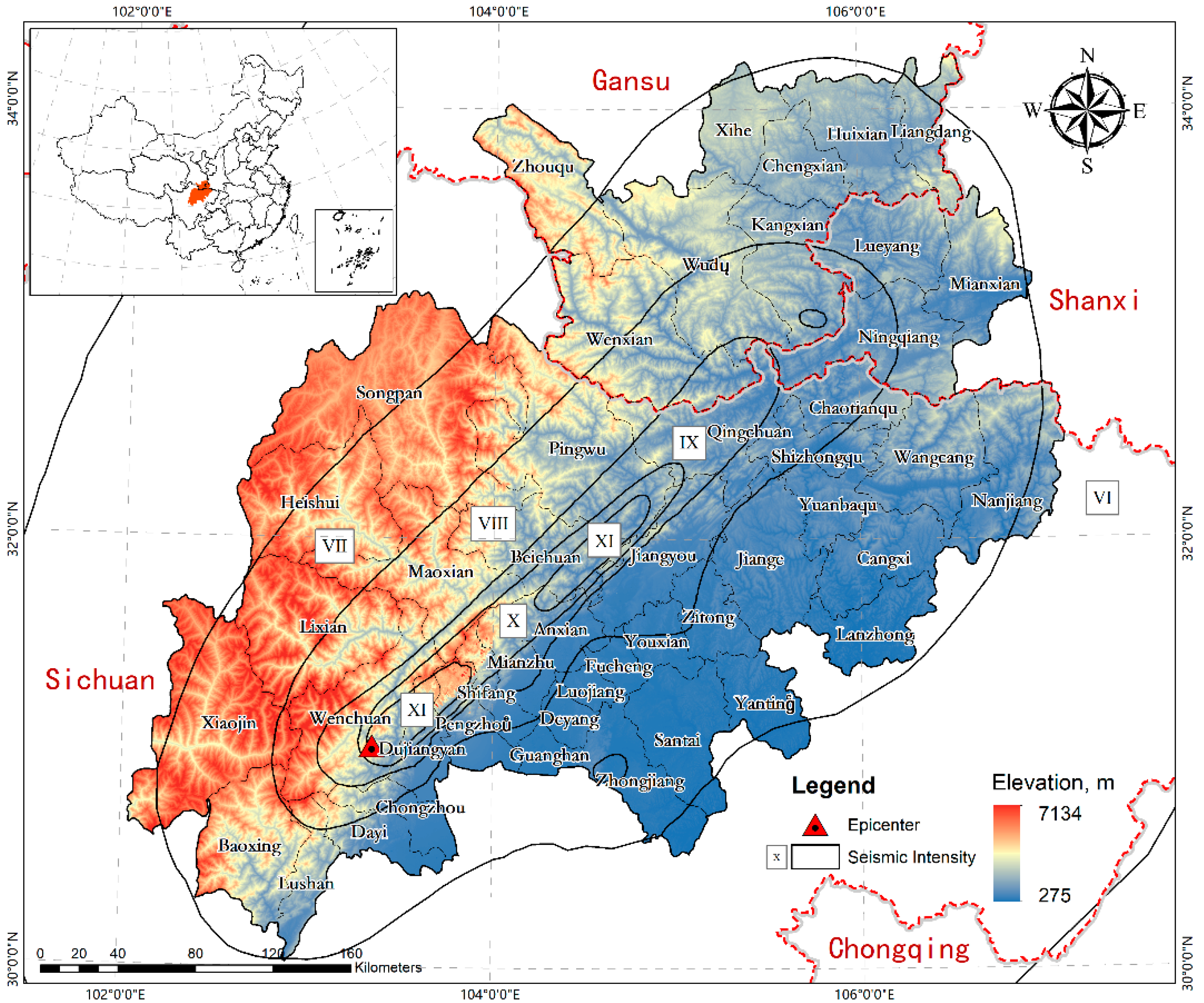
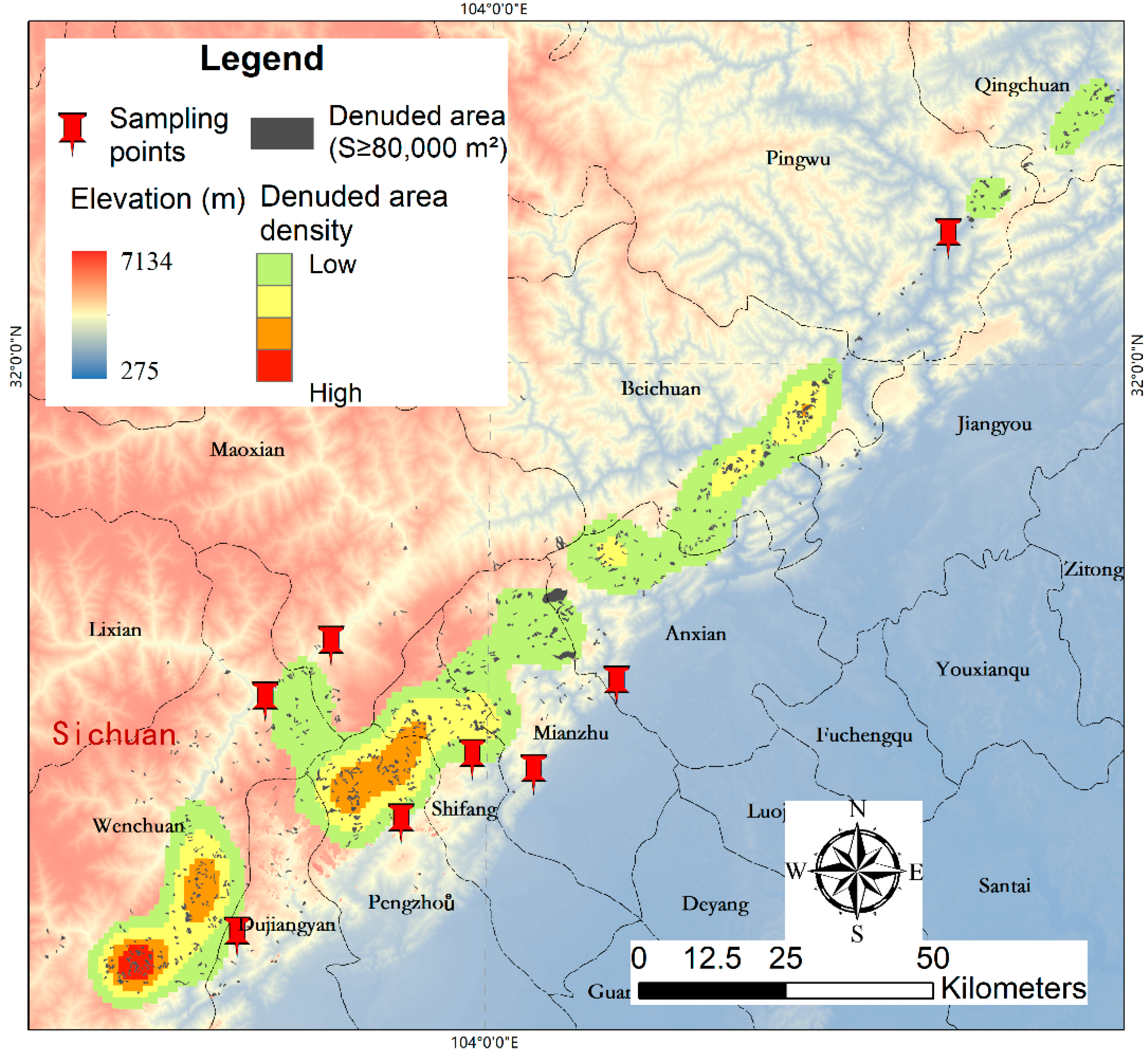
2.1. Study Area
2.2. Data Preparation
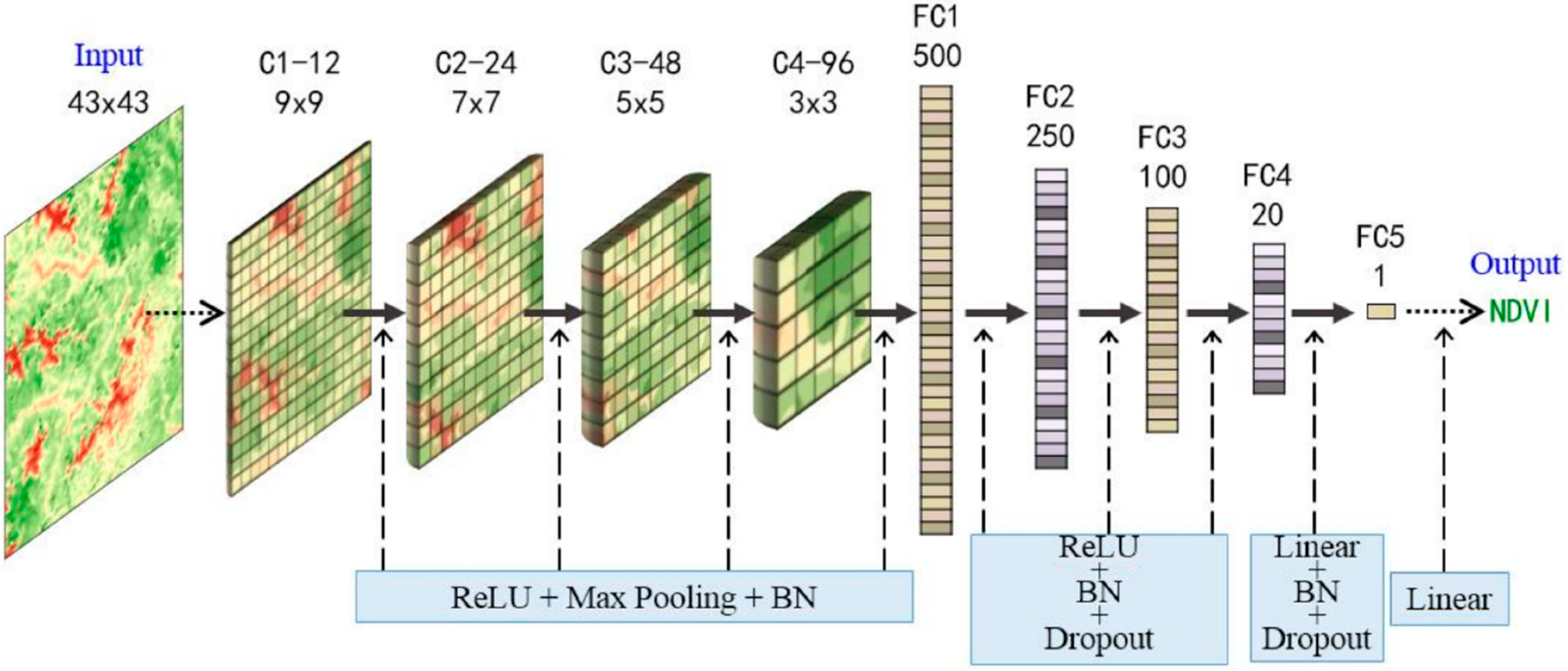
2.3. Convolutional Neural Networks
2.4. Model Evaluation
2.5. Linear Model
2.6. Linear Regression Trend Analysis
2.7. Soil Quality Measurement
2.8. Correlation Measure of Human Activity Intensity and NDVI
3. Results
3.1. Long-Term Series NDVI Reconstruction
3.1.1. Model Evaluation and Data Reconstruction
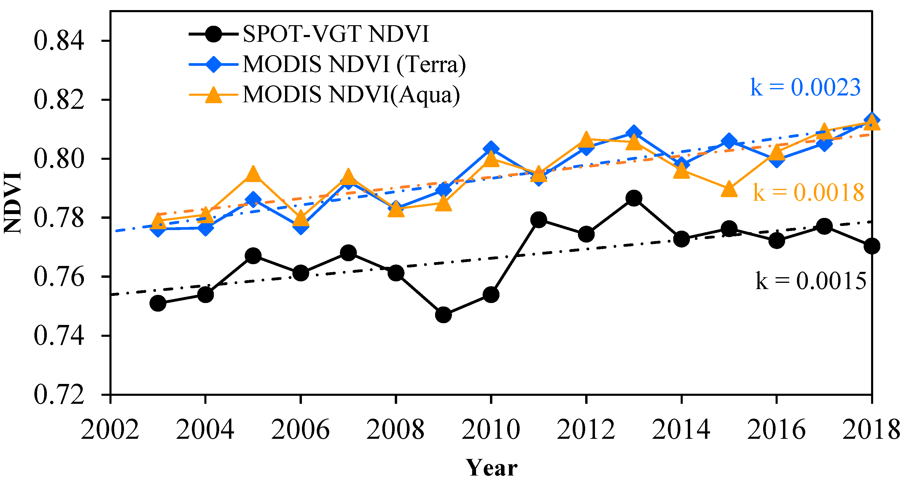
3.1.2. Comparisons to Reconstructed NDVI
3.2. Spatiotemporal Patterns of Vegetation Change
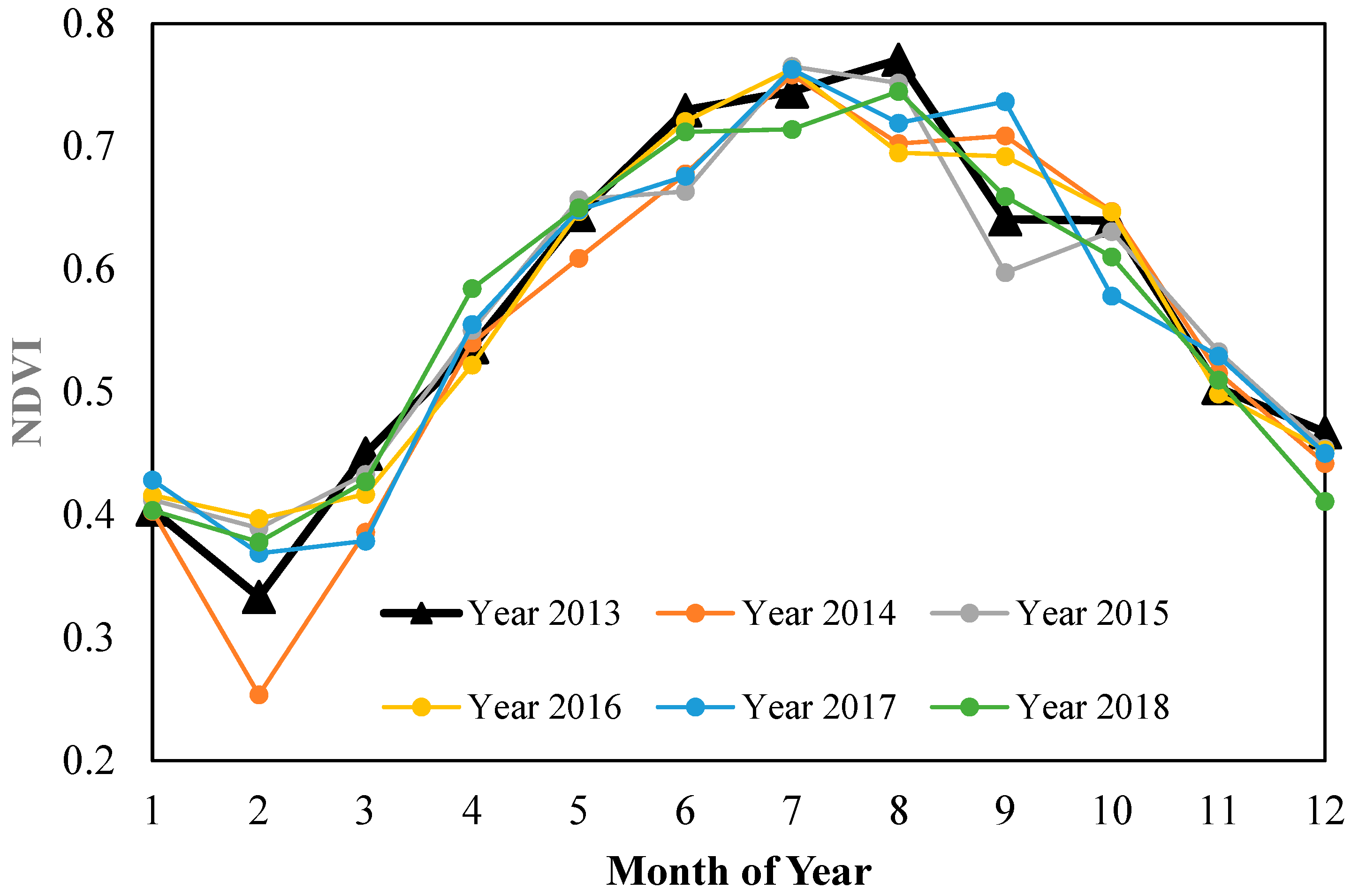
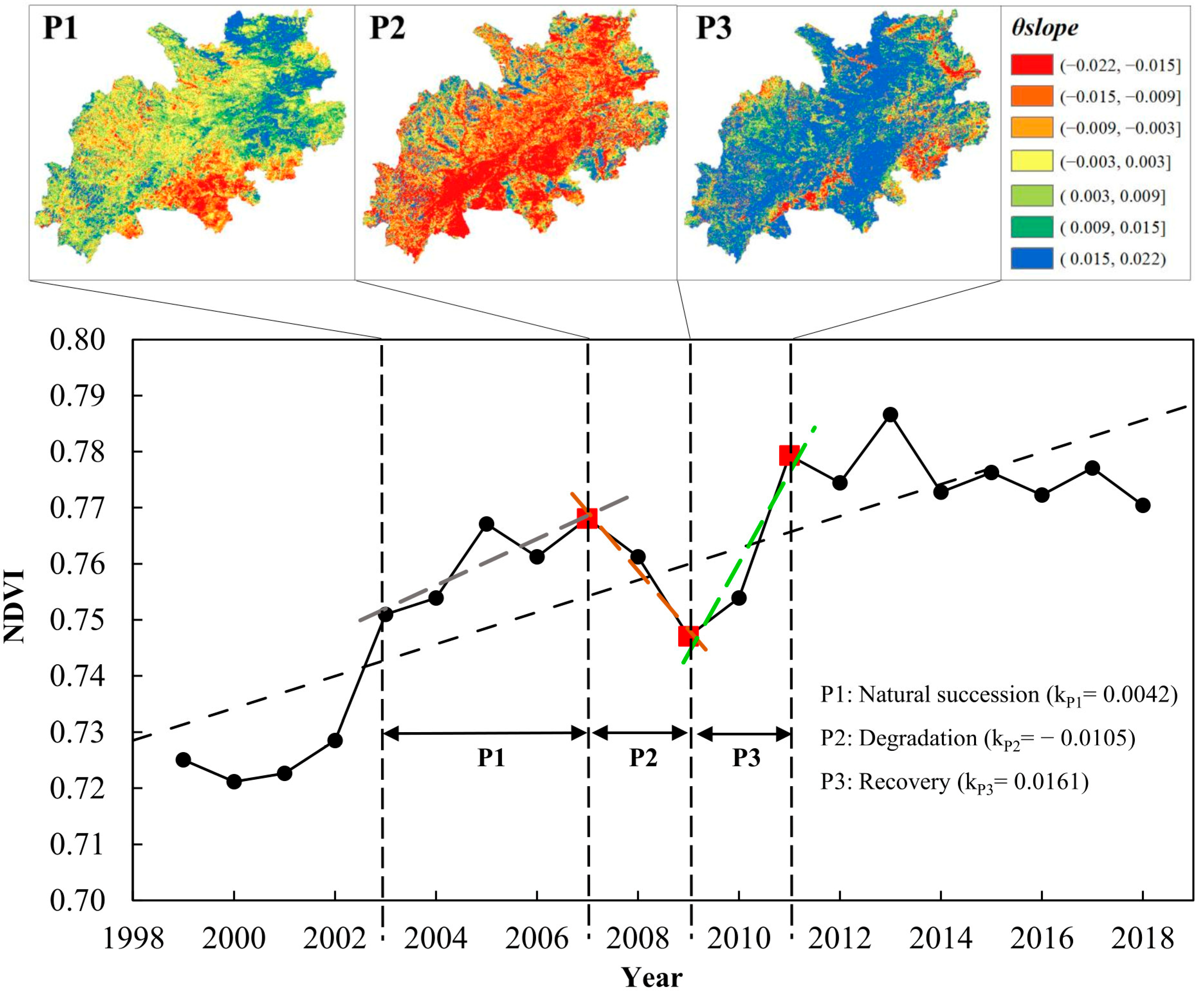
3.2.1. Temporal Patterns
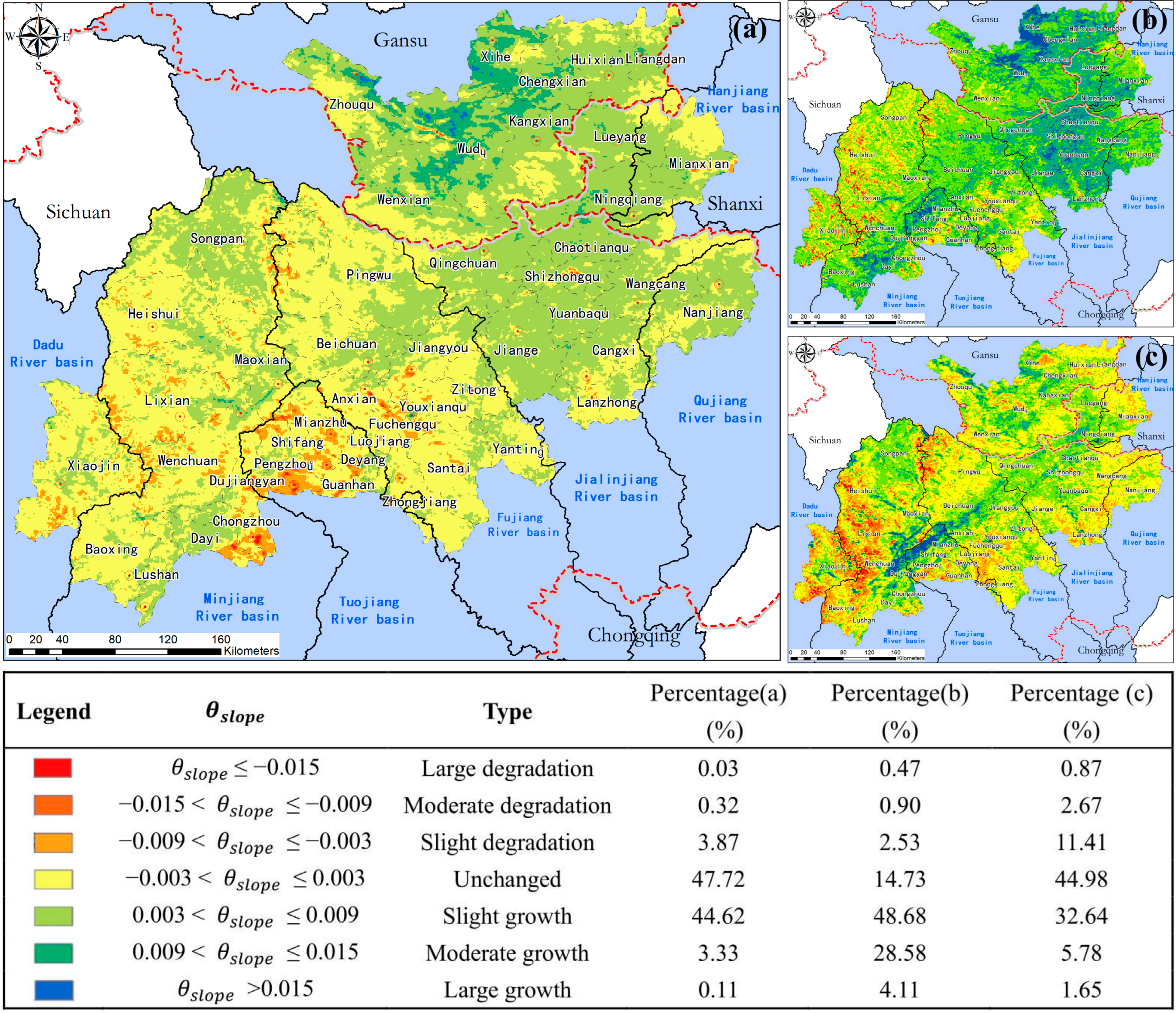
3.2.2. Spatial Distribution of Vegetation Cover
3.3. Vegetation Recovery Patterns after the Earthquake
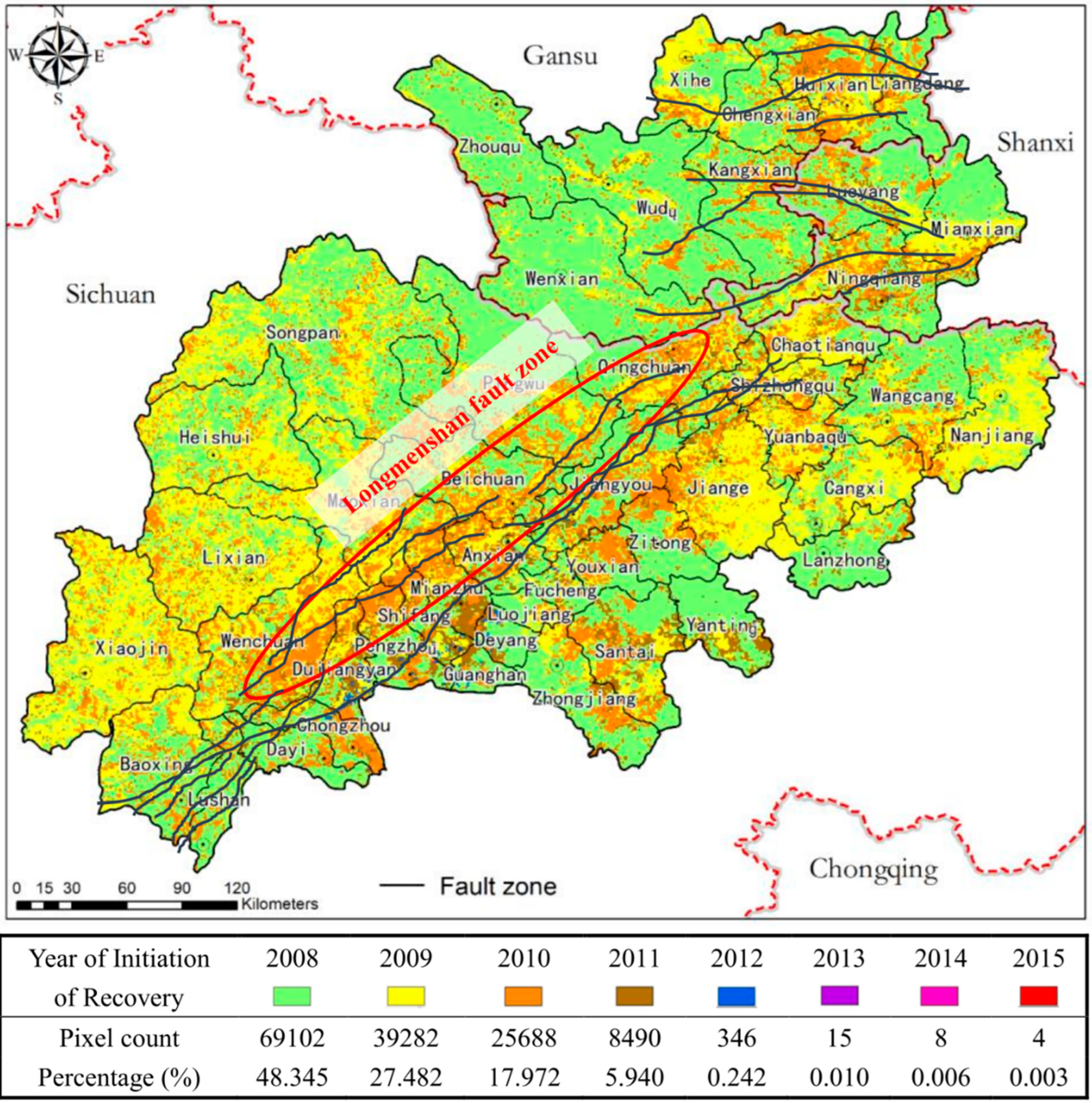
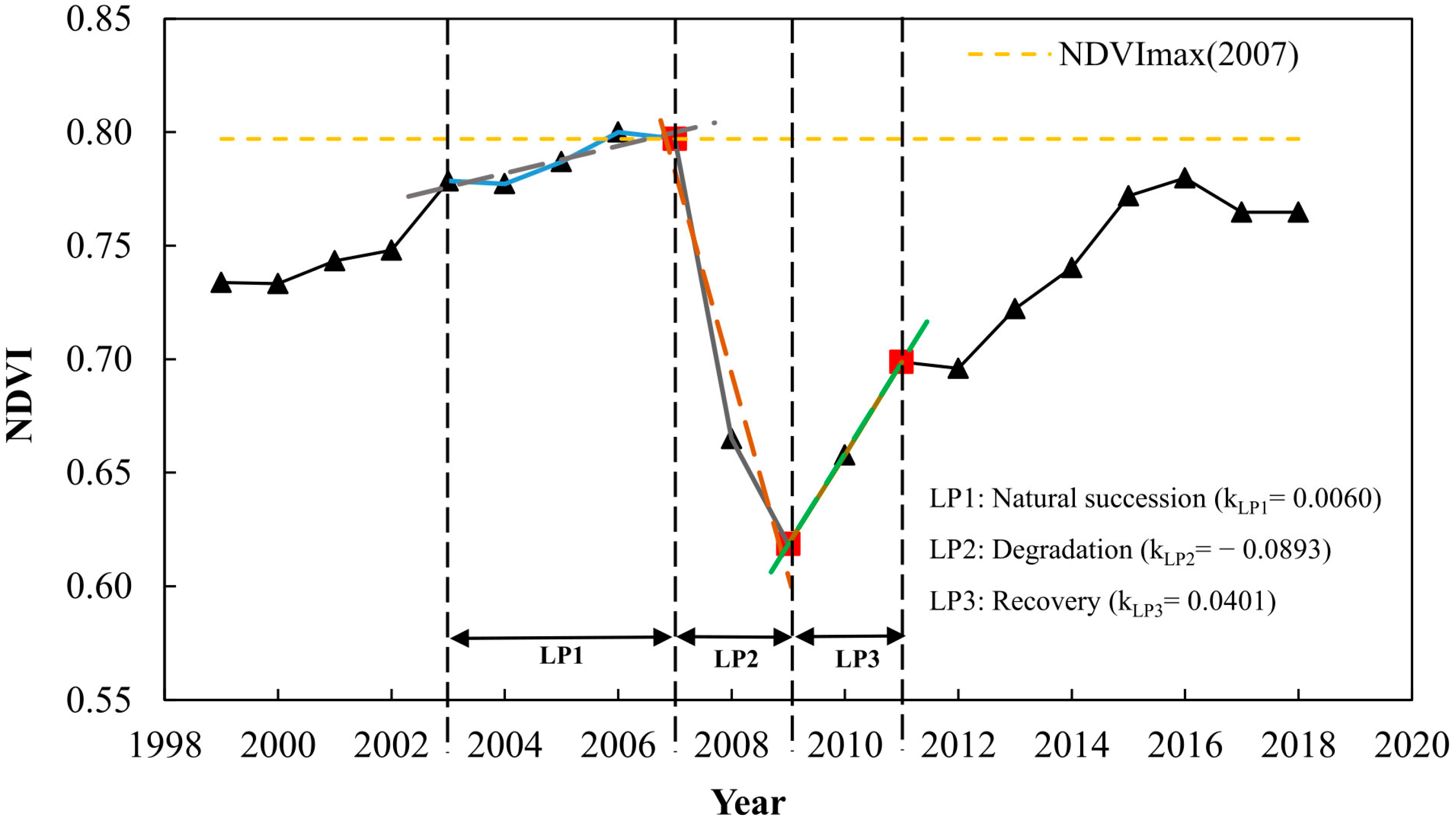
3.3.1. Year of Initiation of Recovery
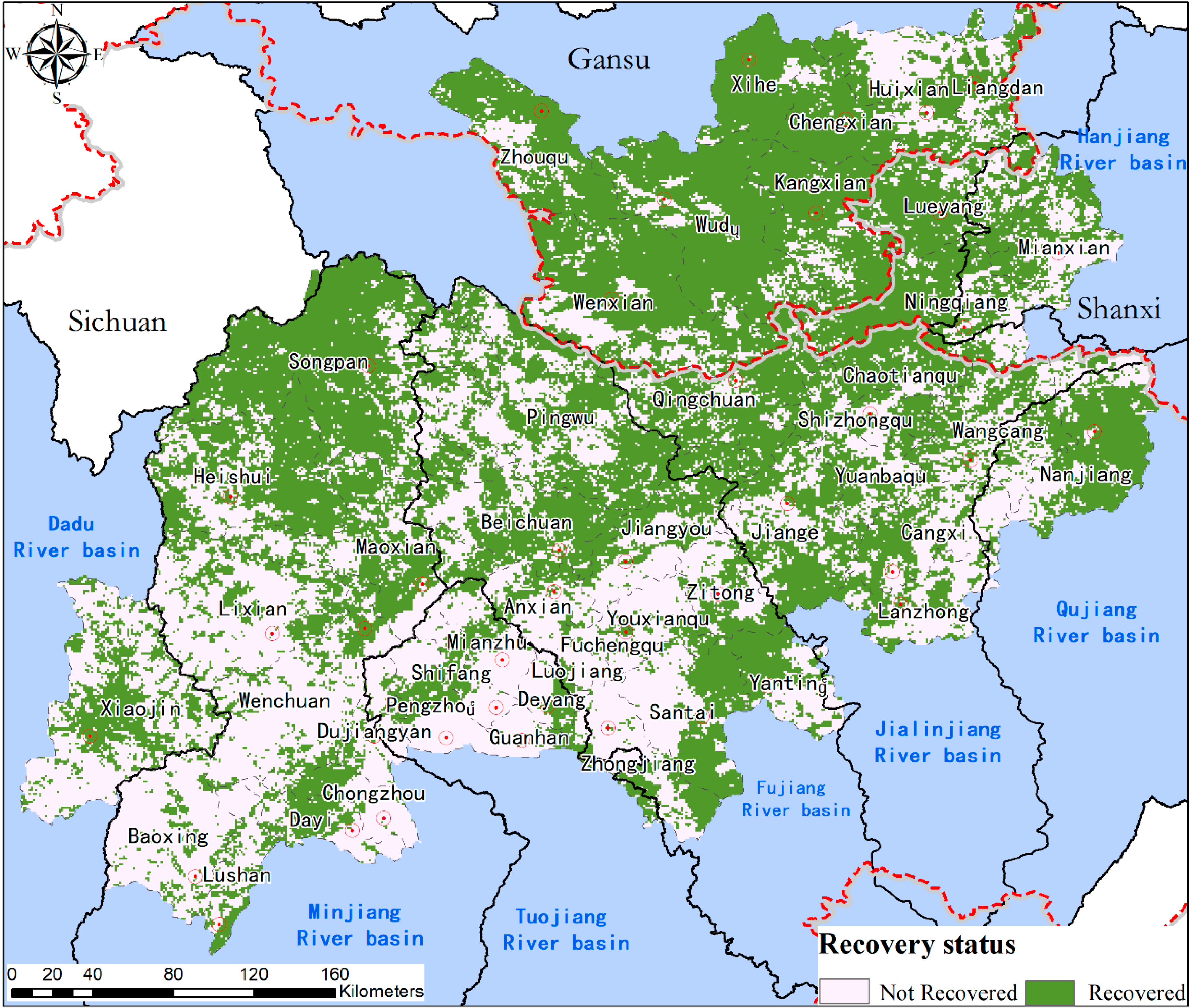
3.3.2. Recovery in the Decade after the Earthquake
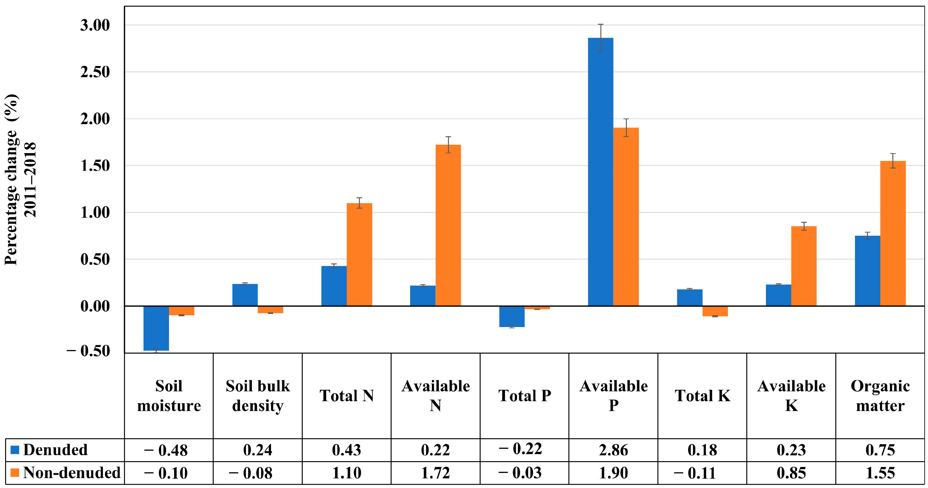
3.3.3. Obstructed Recovery in Denuded Area
3.4. Relationship with Vegetation Change and Other Factors
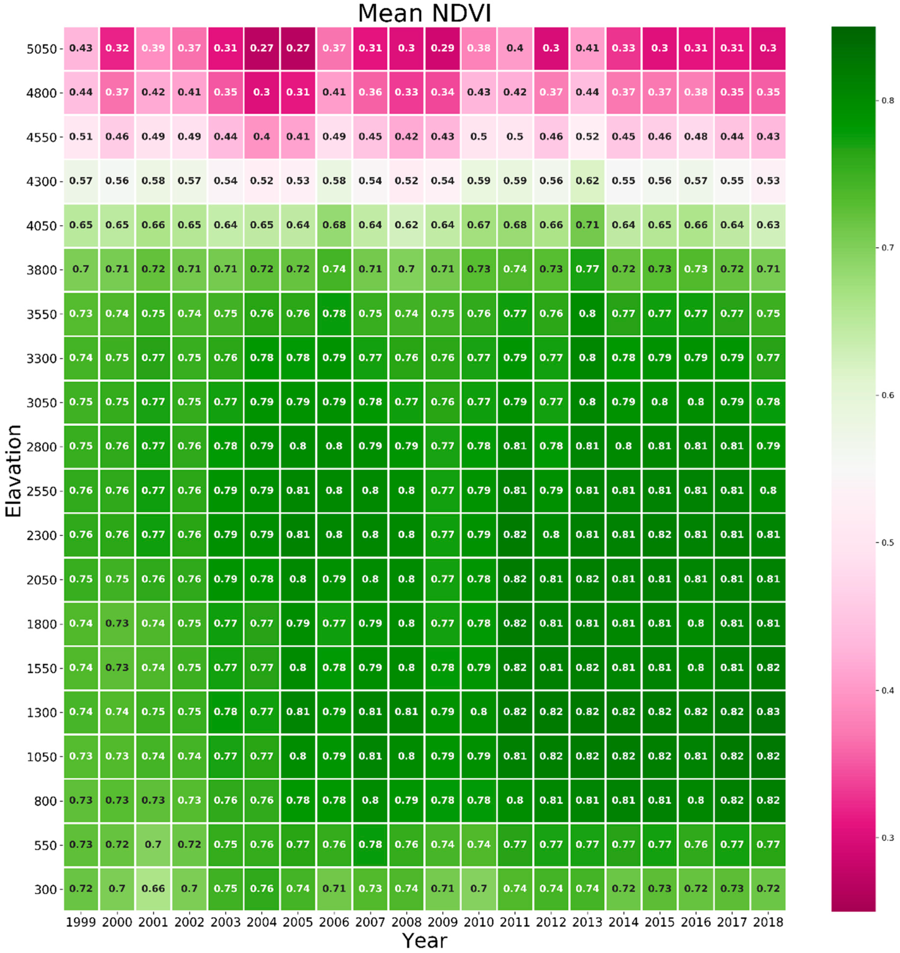
3.4.1. Vegetation Changes in Elevation Belts
3.4.2. Vegetation Change in Different Land Use Types
4. Discussion
5. Conclusions
Supplementary Materials
Author Contributions
Funding
Data Availability Statement
Acknowledgments
Conflicts of Interest
References
- Duan, Y.; Di, B.; Ustin, S.L.; Xu, C.; Xie, Q.; Wu, S.; Li, J.; Zhang, R. Changes in Ecosystem Services in a Montane Landscape Impacted by Major Earthquakes: A Case Study in Wenchuan Earthquake-Affected Area, China. Ecol. Indic. 2021, 126, 107683. [Google Scholar] [CrossRef]
- Marusig, D.; Petruzzellis, F.; Tomasella, M.; Napolitano, R.; Altobelli, A.; Nardini, A. Correlation of Field-Measured and Remotely Sensed Plant Water Status as a Tool to Monitor the Risk of Drought-Induced Forest Decline. Forests 2020, 11, 77. [Google Scholar] [CrossRef]
- Poussin, C.; Massot, A.; Ginzler, C.; Weber, D.; Chatenoux, B.; Lacroix, P.; Piller, T.; Nguyen, L.; Giuliani, G. Drying Conditions in Switzerland—Indication from a 35-Year Landsat Time-Series Analysis of Vegetation Water Content Estimates to Support SDGs. Big Earth Data 2021, 5, 445–475. [Google Scholar] [CrossRef]
- Xu, C.; Xu, X.; Zhou, B.; Yu, G. Revisions of the M 8.0 Wenchuan Earthquake Seismic Intensity Map Based on Co-Seismic Landslide Abundance. Nat. Hazards 2013, 69, 1459–1476. [Google Scholar] [CrossRef]
- Xu, J.; Lu, Y. Meta-Synthesis Pattern of Post-Disaster Recovery and Reconstruction: Based on Actual Investigation on 2008 Wenchuan Earthquake. Nat. Hazards 2012, 60, 199–222. [Google Scholar] [CrossRef]
- Cui, P.; Chen, X.; Zhu, Y.; Su, F.; Wei, F.; Han, Y.-S.; Liu, H.-J.; Zhuang, J.-Q. The Wenchuan Earthquake (May 12, 2008), Sichuan Province, China, and Resulting Geohazards. Nat. Hazards 2011, 56, 19–36. [Google Scholar] [CrossRef]
- Lu, T.; Shi, F.; Sun, G.; Luo, Y.; Wang, Q.; Wu, Y.; Wu, N. Reconstruction of the Wenchuan Earthquake-Damaged Ecosystems: Four Important Questions: Reconstruction of the Wenchuan Earthquake-Damaged Ecosystems: Four Important Questions. Chin. J. Appl. Environ. Biol. 2010, 16, 301–304. [Google Scholar] [CrossRef]
- Pan, K.; Wu, N.; Pan, K.; Chen, Q. A discussion on the issues of the re-construction of ecological shelter zone on the upper reaches of the Yangtze River. Acta Ecol. Sin. 2004, 24, 617–629. [Google Scholar]
- Fan, X.; Domènech, G.; Scaringi, G.; Huang, R.; Xu, Q.; Hales, T.C.; Dai, L.; Yang, Q.; Francis, O. Spatio-Temporal Evolution of Mass Wasting after the 2008 Mw 7.9 Wenchuan Earthquake Revealed by a Detailed Multi-Temporal Inventory. Landslides 2018, 15, 2325–2341. [Google Scholar] [CrossRef]
- Wang, M.; Yang, W.; Shi, P.; Xu, C.; Liu, L. Diagnosis of Vegetation Recovery in Mountainous Regions After the Wenchuan Earthquake. IEEE J. Sel. Top. Appl. Earth Obs. Remote Sens. 2014, 7, 3029–3037. [Google Scholar] [CrossRef]
- Zhang, H.; Chi, T.; Fan, J.; Hu, K.; Peng, L. Spatial Analysis of Wenchuan Earthquake-Damaged Vegetation in the Mountainous Basins and Its Applications. Remote Sens. 2015, 7, 5785–5804. [Google Scholar] [CrossRef]
- Guo, N. Vegetation index and its advances. J. Arid Meteorol. 2003, 21, 71–75. [Google Scholar]
- Tian, Q.; Min, X. Advances in study on vegetation indices. Adv. Earth Sci. 1998, 13, 327–333. [Google Scholar]
- Cihlar, J.; St-Laurent, L.; Dyer, J.A. Relation between the Normalized Difference Vegetation Index and Ecological Variables. Remote Sens. Environ. 1991, 35, 279–298. [Google Scholar] [CrossRef]
- Mbow, C.; Fensholt, R.; Nielsen, T.T.; Rasmussen, K. Advances in Monitoring Vegetation and Land Use Dynamics in the Sahel. Geogr. Tidsskr. Dan. J. Geogr. 2014, 114, 84–91. [Google Scholar] [CrossRef]
- Pettorelli, N.; Vik, J.O.; Mysterud, A.; Gaillard, J.-M.; Tucker, C.J.; Stenseth, N.C. Using the Satellite-Derived NDVI to Assess Ecological Responses to Environmental Change. Trends Ecol. Evol. 2005, 20, 503–510. [Google Scholar] [CrossRef]
- Bradley, B.A.; Mustard, J.F. Comparison of Phenology Trends by Land Cover Class: A Case Study in the Great Basin, USA. Glob. Change Biol. 2008, 14, 334–346. [Google Scholar] [CrossRef]
- Gamon, J.A.; Field, C.B.; Goulden, M.L.; Griffin, K.L.; Hartley, A.E.; Joel, G.; Penuelas, J.; Valentini, R. Relationships Between NDVI, Canopy Structure, and Photosynthesis in Three Californian Vegetation Types. Ecol. Appl. 1995, 5, 28–41. [Google Scholar] [CrossRef]
- Gilabert, M.A.; González-Piqueras, J.; García-Haro, F.J.; Meliá, J. A Generalized Soil-Adjusted Vegetation Index. Remote Sens. Environ. 2002, 82, 303–310. [Google Scholar] [CrossRef]
- Jiang, Z.; Huete, A.R.; Chen, J.; Chen, Y.; Li, J.; Yan, G.; Zhang, X. Analysis of NDVI and Scaled Difference Vegetation Index Retrievals of Vegetation Fraction. Remote Sens. Environ. 2006, 101, 366–378. [Google Scholar] [CrossRef]
- Gitelson, A.A.; Merzlyak, M.N. Remote Estimation of Chlorophyll Content in Higher Plant Leaves. Int. J. Remote Sens. 1997, 18, 2691–2697. [Google Scholar] [CrossRef]
- Myneni, R.B.; Williams, D.L. On the Relationship between FAPAR and NDVI. Remote Sens. Environ. 1994, 49, 200–211. [Google Scholar] [CrossRef]
- Running, S.W.; Nemani, R.R.; Heinsch, F.A.; Zhao, M.; Reeves, M.; Hashimoto, H. A Continuous Satellite-Derived Measure of Global Terrestrial Primary Production. BioScience 2004, 54, 547–560. [Google Scholar] [CrossRef]
- Myneni, R.B.; Hall, F.G.; Sellers, P.J.; Marshak, A.L. The Interpretation of Spectral Vegetation Indexes. IEEE Trans. Geosci. Remote Sens. 1995, 33, 481–486. [Google Scholar] [CrossRef]
- Sellers, P.J. Relations between Canopy Reflectance, Photosynthesis and Transpiration: Links between Optics, Biophysics and Canopy Architecture. Adv. Space Res. 1987, 7, 27–44. [Google Scholar] [CrossRef]
- Sellers, P.J. Canopy Reflectance, Photosynthesis and Transpiration. Int. J. Remote Sens. 1985, 6, 1335–1372. [Google Scholar] [CrossRef]
- Jeong, S.-J.; Schimel, D.; Frankenberg, C.; Drewry, D.T.; Fisher, J.B.; Verma, M.; Berry, J.A.; Lee, J.-E.; Joiner, J. Application of Satellite Solar-Induced Chlorophyll Fluorescence to Understanding Large-Scale Variations in Vegetation Phenology and Function over Northern High Latitude Forests. Remote Sens. Environ. 2017, 190, 178–187. [Google Scholar] [CrossRef]
- Yengoh, G.T.; Dent, D.; Olsson, L.; Tengberg, A.E.; Tucker, C.J., III. Use of the Normalized Difference Vegetation Index (NDVI) to Assess Land Degradation at Multiple Scales: Current Status, Future Trends, and Practical Considerations; Springer: Berlin/Heidelberg, Germany, 2015; ISBN 978-3-319-24112-8. [Google Scholar]
- Cao, M.; Prince, S.D.; Li, K.; Tao, B.; Small, J.; Shao, X. Response of Terrestrial Carbon Uptake to Climate Interannual Variability in China. Glob. Change Biol. 2003, 9, 536–546. [Google Scholar] [CrossRef]
- Field, C.B.; Randerson, J.T.; Malmström, C.M. Global Net Primary Production: Combining Ecology and Remote Sensing. Remote Sens. Environ. 1995, 51, 74–88. [Google Scholar] [CrossRef]
- Gamon, J.A.; Huemmrich, K.F.; Stone, R.S.; Tweedie, C.E. Spatial and Temporal Variation in Primary Productivity (NDVI) of Coastal Alaskan Tundra: Decreased Vegetation Growth Following Earlier Snowmelt. Remote Sens. Environ. 2013, 129, 144–153. [Google Scholar] [CrossRef]
- Wang, R.; Gamon, J.A.; Emmerton, C.A.; Li, H.; Nestola, E.; Pastorello, G.Z.; Menzer, O. Integrated Analysis of Productivity and Biodiversity in a Southern Alberta Prairie. Remote Sens. 2016, 8, 214. [Google Scholar] [CrossRef]
- Albarakat, R.; Lakshmi, V. Comparison of Normalized Difference Vegetation Index Derived from Landsat, MODIS, and AVHRR for the Mesopotamian Marshes Between 2002 and 2018. Remote Sens. 2019, 11, 1245. [Google Scholar] [CrossRef]
- Bright, B.C.; Hudak, A.T.; Kennedy, R.E.; Braaten, J.D.; Henareh Khalyani, A. Examining Post-Fire Vegetation Recovery with Landsat Time Series Analysis in Three Western North American Forest Types. Fire Ecol. 2019, 15, 8. [Google Scholar] [CrossRef]
- Díaz-Delgado, R.; Lloret, F.; Pons, X. Influence of Fire Severity on Plant Regeneration by Means of Remote Sensing Imagery. Int. J. Remote Sens. 2003, 24, 1751–1763. [Google Scholar] [CrossRef]
- Fensholt, R.; Rasmussen, K.; Nielsen, T.T.; Mbow, C. Evaluation of Earth Observation Based Long Term Vegetation Trends—Intercomparing NDVI Time Series Trend Analysis Consistency of Sahel from AVHRR GIMMS, Terra MODIS and SPOT VGT Data. Remote Sens. Environ. 2009, 113, 1886–1898. [Google Scholar] [CrossRef]
- Karnieli, A.; Agam, N.; Pinker, R.T.; Anderson, M.; Imhoff, M.L.; Gutman, G.G.; Panov, N.; Goldberg, A. Use of NDVI and Land Surface Temperature for Drought Assessment: Merits and Limitations. J. Clim. 2010, 23, 618–633. [Google Scholar] [CrossRef]
- Shi, L.; Dech, J.; Liu, H.; Zhao, P.; Bayin, D.; Zhou, M. Post-fire Vegetation Recovery at Forest Sites Is Affected by Permafrost Degradation in the Da Xing’an Mountains of Northern China. J. Veg. Sci. 2019, 30, 940–949. [Google Scholar] [CrossRef]
- Brown, M.; Lary, D.; Vrieling, A.; Stathakis, D.; Mussa, H. Neutral Networks as a Tool for Constructing Continuous NDVI Time Series from AVHRR and MODIS. Int. J. Remote Sens. 2008, 29, 7141. [Google Scholar] [CrossRef]
- Gallo, K.; Ji, L.; Reed, B.; Eidenshink, J.; Dwyer, J. Multi-Platform Comparisons of MODIS and AVHRR Normalized Difference Vegetation Index Data. Remote Sens. Environ. 2005, 99, 221–231. [Google Scholar] [CrossRef]
- Song, Y.; Mingguo, M.; Veroustraete, F. Comparison and Conversion of AVHRR GIMMS and SPOT VEGETATION NDVI Data in China. Int. J. Remote Sens. 2010, 31, 2377–2392. [Google Scholar] [CrossRef]
- Tarnavsky, E.; Garrigues, S.; Brown, M. Multiscale Geostatistical Analysis of AVHRR, SPOT-VGT, and MODIS Global NDVI Products. Remote Sens. Environ. 2008, 112, 535–549. [Google Scholar] [CrossRef]
- Ni, Z.; Yang, Z.; Li, W.; Zhao, Y.; He, Z. Decreasing Trend of Geohazards Induced by the 2008 Wenchuan Earthquake Inferred from Time Series NDVI Data. Remote Sens. 2019, 11, 2192. [Google Scholar] [CrossRef]
- Yunus, A.P.; Fan, X.; Tang, X.; Jie, D.; Xu, Q.; Huang, R. Decadal Vegetation Succession from MODIS Reveals the Spatio-Temporal Evolution of Post-Seismic Landsliding after the 2008 Wenchuan Earthquake. Remote Sens. Environ. 2020, 236, 111476. [Google Scholar] [CrossRef]
- Zhang, W.; Lin, J.; Peng, J.; Lu, Q. Estimating Wenchuan Earthquake Induced Landslides Based on Remote Sensing. Int. J. Remote Sens. 2010, 31, 3495–3508. [Google Scholar] [CrossRef]
- Liu, X. Vegetation Indices Based on Different Sources of Remote Sensing Data Analyzed in Qinling Region. Master’s Thesis, Chang`an University, Xi`an, China, 2015. [Google Scholar]
- An, Y.; Gao, W.; Gao, Z.; Liu, C.; Shi, R. Trend Analysis for Evaluating the Consistency of Terra MODIS and SPOT VGT NDVI Time Series Products in China. Front. Earth Sci. 2015, 9, 125–136. [Google Scholar] [CrossRef]
- Chen, J.; Jönsson, P.; Tamura, M.; Gu, Z.; Matsushita, B.; Eklundh, L. A Simple Method for Reconstructing a High-Quality NDVI Time-Series Data Set Based on the Savitzky–Golay Filter. Remote Sens. Environ. 2004, 91, 332–344. [Google Scholar] [CrossRef]
- Savitzky, A.; Golay, M.J.E. Smoothing and Differentiation of Data by Simplified Least Squares Procedures. Anal. Chem. 1964, 36, 1627–1639. [Google Scholar] [CrossRef]
- Beck, P.S.A.; Atzberger, C.; Høgda, K.A.; Johansen, B.; Skidmore, A.K. Improved Monitoring of Vegetation Dynamics at Very High Latitudes: A New Method Using MODIS NDVI. Remote Sens. Environ. 2006, 100, 321–334. [Google Scholar] [CrossRef]
- Roerink, G.J.; Menenti, M.; Verhoef, W. Reconstructing Cloudfree NDVI Composites Using Fourier Analysis of Time Series. Int. J. Remote Sens. 2000, 21, 1911–1917. [Google Scholar] [CrossRef]
- Das, M.; Ghosh, S.K. A Deep-Learning-Based Forecasting Ensemble to Predict Missing Data for Remote Sensing Analysis. IEEE J. Sel. Top. Appl. Earth Obs. Remote Sens. 2017, 10, 5228–5236. [Google Scholar] [CrossRef]
- Dardel, C.; Kergoat, L.; Hiernaux, P.; Mougin, E.; Manuela, G.; Tucker, C. Re-Greening Sahel: 30 Years of Remote Sensing Data and Field Observations (Mali, Niger). Remote Sens. Environ. 2014, 140, 350–364. [Google Scholar] [CrossRef]
- Van Leeuwen, W.; Orr, B.J.; Marsh, S.; Herrmann, S. Multi-Sensor NDVI Data Continuity: Uncertainties and Implications for Vegetation Monitoring Applications. Remote Sens. Environ. 2006, 100, 67–81. [Google Scholar] [CrossRef]
- Wang, L.; Qu, J.J.; Xiong, X.; Hao, X.; Xie, Y.; Che, N. A New Method for Retrieving Band 6 of Aqua MODIS. IEEE Geosci. Remote Sens. Lett. 2006, 3, 267–270. [Google Scholar] [CrossRef]
- Boyte, S.P.; Wylie, B.K.; Rigge, M.B.; Dahal, D. Fusing MODIS with Landsat 8 Data to Downscale Weekly Normalized Difference Vegetation Index Estimates for Central Great Basin Rangelands, USA. GIScience Remote Sens. 2018, 55, 376–399. [Google Scholar] [CrossRef]
- Wei, J.; Wang, L.; Liu, P.; Chen, X.; Li, W.; Zomaya, A.Y. Spatiotemporal Fusion of MODIS and Landsat-7 Reflectance Images via Compressed Sensing. IEEE Trans. Geosci. Remote Sens. 2017, 55, 7126–7139. [Google Scholar] [CrossRef]
- Shen, H.; Li, X.; Cheng, Q.; Zeng, C.; Yang, G.; Li, H.; Zhang, L. Missing Information Reconstruction of Remote Sensing Data: A Technical Review. IEEE Geosci. Remote Sens. Mag. 2015, 3, 61–85. [Google Scholar] [CrossRef]
- Li, S.; Xu, L.; Jing, Y.; Yin, H.; Li, X.; Guan, X. High-Quality Vegetation Index Product Generation: A Review of NDVI Time Series Reconstruction Techniques. Int. J. Appl. Earth Obs. Geoinf. 2021, 105, 102640. [Google Scholar] [CrossRef]
- Zhang, Q.; Yuan, Q.; Zeng, C.; Li, X.; Wei, Y. Missing Data Reconstruction in Remote Sensing Image with a Unified Spatial–Temporal–Spectral Deep Convolutional Neural Network. IEEE Trans. Geosci. Remote Sens. 2018, 56, 4274–4288. [Google Scholar] [CrossRef]
- Zhang, Q.; Yuan, Q.; Li, J.; Li, Z.; Shen, H.; Zhang, L. Thick Cloud and Cloud Shadow Removal in Multitemporal Imagery Using Progressively Spatio-Temporal Patch Group Deep Learning. ISPRS J. Photogramm. Remote Sens. 2020, 162, 148–160. [Google Scholar] [CrossRef]
- Xu, T.; Wang, Y.; Fu, B. Evaluation on sensibility of soil erosion of harder-hit area of Wenchuan Earthquake. Soil Water Conserv. China 2011, 1, 39–42+67. [Google Scholar] [CrossRef]
- Wolters, E.; Dierckx, W.; Iordache, M.-D.; Swinnen, E. PROBA-V Products User Manual v3.01. 2018.
- Jiao, Q.; Liu, L.; Li, Z.; Yue, Y.; Hu, Y. Assessment of Spatio-Temporal Variations in Vegetation Recovery after the Wenchuan Earthquake Using Landsat Data. Nat. Hazards 2014, 70, 1309–1326. [Google Scholar] [CrossRef]
- Yu, S.; Liu, J.; Yuan, J. Vegetation Change of Yamzho Yumco Basin in Southern Tibet Based on SPOT-VGT NDVI. Spectrosc. Spectr. Anal. 2010, 30, 1570–1574. [Google Scholar] [CrossRef]
- Sun, J. 1982~2000 Vegetation Change in China and Response of Typical Areas with Climatic Factors. Master’s Thesis, Nanjing University of Information Science & Technology, Nanjing, China, 2007. [Google Scholar]
- Yuan, Q.; Shen, H.; Li, T.; Li, Z.; Li, S.; Jiang, Y.; Xu, H.; Tan, W.; Yang, Q.; Wang, J.; et al. Deep Learning in Environmental Remote Sensing: Achievements and Challenges. Remote Sens. Environ. 2020, 241, 111716. [Google Scholar] [CrossRef]
- Muhammad, K.; Ahmad, J.; Baik, S.W. Early Fire Detection Using Convolutional Neural Networks during Surveillance for Effective Disaster Management. Neurocomputing 2018, 288, 30–42. [Google Scholar] [CrossRef]
- Huang, B.; Zhao, B.; Song, Y. Urban Land-Use Mapping Using a Deep Convolutional Neural Network with High Spatial Resolution Multispectral Remote Sensing Imagery. Remote Sens. Environ. 2018, 214, 73–86. [Google Scholar] [CrossRef]
- Shimobaba, T.; Kakue, T.; Ito, T. Convolutional Neural Network-Based Regression for Depth Prediction in Digital Holography. In Proceedings of the 2018 IEEE 27th International Symposium on Industrial Electronics (ISIE), Cairns, Qld, Australia, 13–15 June 2018; pp. 1323–1326. [Google Scholar] [CrossRef]
- Zhang, R.; Di, B.; Luo, Y.; Deng, X.; Grieneisen, M.L.; Wang, Z.; Yao, G.; Zhan, Y. A Nonparametric Approach to Filling Gaps in Satellite-Retrieved Aerosol Optical Depth for Estimating Ambient PM2.5 Levels. Environ. Pollut. 2018, 243, 998–1007. [Google Scholar] [CrossRef]
- Stow, D.; Daeschner, S.; Hope, A.; Douglas, D.; Petersen, A.; Myneni, R.; Zhou, L.; Oechel, W. Variability of the Seasonally Integrated Normalized Difference Vegetation Index Across the North Slope of Alaska in the 1990s. Int. J. Remote Sens. 2003, 24, 1111–1117. [Google Scholar] [CrossRef]
- Gao, X.; Huete, A.R.; Ni, W.; Miura, T. Optical–Biophysical Relationships of Vegetation Spectra without Background Contamination. Remote Sens. Environ. 2000, 74, 609–620. [Google Scholar] [CrossRef]
- Wan, X. Vegetation Restoration and Its Effects on Soil after Converting Agricultural Lands to Forest. Master’s Thesis, Sichuan Agricultural University, Yaan, China, 2003. [Google Scholar]
- Xie, Y.; Shao, Z.; Lan, X.; Li, F.; Zeng, F. Relationship Between Land Use and Soil Erosion in Karst Area-A Case Study of Bijie Experimental Area. Res. Soil Water Conserv. 2017, 24, 1–5. [Google Scholar] [CrossRef]
- Tian, F.; Fensholt, R.; Verbesselt, J.; Grogan, K.; Horion, S.; Wang, Y. Evaluating Temporal Consistency of Long-Term Global NDVI Datasets for Trend Analysis. Remote Sens. Environ. 2015, 163, 326–340. [Google Scholar] [CrossRef]
- Hong, Y.; Zhao, Y.; Wang, Y.; Xin, C.; Zhao, Y. Temporal and Spatial Variation Characteristics of Vegetation Restoration Based on MODIS-NDVI Wenchuan Earthquake Region in Ten Years. Sci. Technol. Eng. 2019, 19, 64–74. [Google Scholar]
- Li, J.; Cao, M.; Qiu, H.; Xue, B.; Hu, S.; Cui, P. Spatial-temporal process and characteristics of vegetation recovery after Wenchuan earthquake: A case study in Longxi River basin of Dujiangyan, China. Chin. J. Appl. Ecol. 2016, 27, 3479–3486. [Google Scholar] [CrossRef]
- Chen, N.; Lu, Y.; Zhou, H.; Deng, M.; Han, D. Combined Impacts of Antecedent Earthquakes and Droughts on Disastrous Debris Flows. J. Mt. Sci. 2014, 11, 1507–1520. [Google Scholar] [CrossRef]
- Di, B.; Zhang, H.; Liu, Y.; Li, J.; Chen, N.; Stamatopoulos, C.A.; Luo, Y.; Zhan, Y. Assessing Susceptibility of Debris Flow in Southwest China Using Gradient Boosting Machine. Sci. Rep. 2019, 9, 12532. [Google Scholar] [CrossRef]
- Jiang, W.-G.; Jia, K.; Wu, J.-J.; Tang, Z.-H.; Wang, W.-J.; Liu, X.-F. Evaluating the Vegetation Recovery in the Damage Area of Wenchuan Earthquake Using MODIS Data. Remote Sens. 2015, 7, 8757–8778. [Google Scholar] [CrossRef]
- Cui, P. Atlas of Mountain Hazards and Soil Erosion in the Upper Yangtze; Science Press: Beijing, China, 2014. [Google Scholar]
- Xu, C. Detailed Inventory of Landslides Triggered by the 2008 Wenchuan Earthquake and Its Comparison with Other Earthquake Events in the World. Sci. Technol. Rev. 2012, 30, 18–26. [Google Scholar]
- Liu, Y.; Liu, R.; Ge, Q. Evaluating the Vegetation Destruction and Recovery of Wenchuan Earthquake Using MODIS Data. Nat. Hazards 2010, 54, 851–862. [Google Scholar] [CrossRef]
- Cui, P.; Lin, Y.; Chen, C. Destruction of Vegetation Due to Geo-Hazards and Its Environmental Impacts in the Wenchuan Earthquake Areas. Ecol. Eng. 2012, 44, 61–69. [Google Scholar] [CrossRef]
- Yang, W.; Qi, W.; Zhou, J. Decreased Post-Seismic Landslides Linked to Vegetation Recovery after the 2008 Wenchuan Earthquake. Ecol. Indic. 2018, 89, 438–444. [Google Scholar] [CrossRef]
- Chen, M.; Tang, C.; Xiong, J.; Shi, Q.Y.; Li, N.; Gong, L.F.; Wang, X.D.; Tie, Y. The Long-Term Evolution of Landslide Activity near the Epicentral Area of the 2008 Wenchuan Earthquake in China. Geomorphology 2020, 367, 107317. [Google Scholar] [CrossRef]
- Zhong, C.; Li, C.; Gao, P.; Li, H. Discovering Vegetation Recovery and Landslide Activities in the Wenchuan Earthquake Area with Landsat Imagery. Sensors 2021, 21, 5243. [Google Scholar] [CrossRef] [PubMed]
- Baldi, G.; Nosetto, M.D.; Aragón, R.; Aversa, F.; Paruelo, J.M.; Jobbágy, E.G. Long-Term Satellite NDVI Data Sets: Evaluating Their Ability to Detect Ecosystem Functional Changes in South America. Sensors 2008, 8, 5397–5425. [Google Scholar] [CrossRef] [PubMed]
- Shen, P.; Zhang, L.M.; Fan, R.L.; Zhu, H.; Zhang, S. Declining Geohazard Activity with Vegetation Recovery during First Ten Years after the 2008 Wenchuan Earthquake. Geomorphology 2020, 352, 106989. [Google Scholar] [CrossRef]
- Hu, G.; Chen, N.; Tanoli, J.I.; Liu, M.; Liu, R.-K.; Chen, K.-T. Debris Flow Susceptibility Analysis Based on the Combined Impacts of Antecedent Earthquakes and Droughts: A Case Study for Cascade Hydropower Stations in the Upper Yangtze River, China. J. Mt. Sci. 2017, 14, 1712–1727. [Google Scholar] [CrossRef]


| NDVI Dataset | Spatial Resolution | Time Range | Data Type | Data Source |
|---|---|---|---|---|
| Original SPOT-VGT | 1 km | 1998.04–2014.05 | HDF4 | https://www.vito-eodata.be/PDF/portal/Application.html#Home (accessed on 12 May 2022) |
| PROBA-V | 1 km | 2013.11–2018.12 | TIFF | https://www.vito-eodata.be/PDF/portal/Application.html#Home (accessed on 12 May 2022) |
| MYD13A2 | 1 km | 2003.01–2018.12 | HDF | https://ladsweb.modaps.eosdis.nasa.gov/ (accessed on 12 May 2022) |
| MOD13A3 | 1 km | 2003.01–2018.12 | HDF | https://ladsweb.modaps.eosdis.nasa.gov/ (accessed on 12 May 2022) |
| Date Index | Model | 2013-11 | 2013-12 | 2014-01 | 2014-02 | 2014-03 | 2014-04 | 2014-05 |
|---|---|---|---|---|---|---|---|---|
| R2 | CNNs | 0.884 | 0.846 | 0.857 | 0.790 | 0.796 | 0.776 | 0.781 |
| Linear | 0.783 | 0.756 | 0.748 | 0.722 | 0.714 | 0.723 | 0.721 | |
| Slope | CNNs | 0.886 | 0.889 | 0.879 | 0.764 | 0.899 | 0.819 | 0.836 |
| Linear | 0.794 | 0.778 | 0.764 | 0.664 | 0.776 | 0.780 | 0.774 | |
| Min Bias * | CNNs | 0.027 | 0.048 | −0.04 | −0.037 | 0.065 | 0.02 | −0.013 |
| Linear | 0.109 | 0.108 | 0.106 | 0.126 | 0.111 | 0.070 | 0.071 | |
| Max Bias * | CNNs | 0.03 | −0.002 | −0.056 | −0.025 | −0.006 | −0.079 | −0.024 |
| Linear | −0.109 | −0.106 | −0.108 | −0.113 | −0.092 | −0.105 | −0.100 |
Disclaimer/Publisher’s Note: The statements, opinions and data contained in all publications are solely those of the individual author(s) and contributor(s) and not of MDPI and/or the editor(s). MDPI and/or the editor(s) disclaim responsibility for any injury to people or property resulting from any ideas, methods, instructions or products referred to in the content. |
© 2023 by the authors. Licensee MDPI, Basel, Switzerland. This article is an open access article distributed under the terms and conditions of the Creative Commons Attribution (CC BY) license (https://creativecommons.org/licenses/by/4.0/).
Share and Cite
Wu, S.; Di, B.; Ustin, S.L.; Wong, M.S.; Adhikari, B.R.; Zhang, R.; Luo, M. Dynamic Characteristics of Vegetation Change Based on Reconstructed Heterogenous NDVI in Seismic Regions. Remote Sens. 2023, 15, 299. https://doi.org/10.3390/rs15020299
Wu S, Di B, Ustin SL, Wong MS, Adhikari BR, Zhang R, Luo M. Dynamic Characteristics of Vegetation Change Based on Reconstructed Heterogenous NDVI in Seismic Regions. Remote Sensing. 2023; 15(2):299. https://doi.org/10.3390/rs15020299
Chicago/Turabian StyleWu, Shaolin, Baofeng Di, Susan L. Ustin, Man Sing Wong, Basanta Raj Adhikari, Ruixin Zhang, and Maoting Luo. 2023. "Dynamic Characteristics of Vegetation Change Based on Reconstructed Heterogenous NDVI in Seismic Regions" Remote Sensing 15, no. 2: 299. https://doi.org/10.3390/rs15020299
APA StyleWu, S., Di, B., Ustin, S. L., Wong, M. S., Adhikari, B. R., Zhang, R., & Luo, M. (2023). Dynamic Characteristics of Vegetation Change Based on Reconstructed Heterogenous NDVI in Seismic Regions. Remote Sensing, 15(2), 299. https://doi.org/10.3390/rs15020299